ReFuse: Generating Imperviousness Maps from Multi-Spectral Sentinel-2 Satellite Imagery

Abstract

Continual mapping and monitoring of impervious surfaces are crucial activities to support sustainable urban management strategies and to plan effective actions for environmental changes. In this context, impervious surface coverage is increasingly becoming an essential indicator for assessing urbanization and environmental quality, with several works relying on satellite imagery to determine it. However, although satellite imagery is typically available with a frequency of 3–10 days worldwide, imperviousness maps are released at most annually as they require a huge human effort to be produced and validated. Attempts have been made to extract imperviousness maps from satellite images using machine learning, but (i) the scarcity of reliable and detailed ground truth (ii) together with the need to manage different spectral bands (iii) while making the resulting system easily accessible to the end users is limiting their diffusion. To tackle these problems, in this work we introduce a deep-learning-based approach to extract imperviousness maps from multi-spectral Sentinel-2 images leveraging a very detailed imperviousness map realised by the Italian department for environment protection as ground truth. We also propose a scalable and portable inference pipeline designed to easily scale the approach, integrating it into a web-based Geographic Information System (GIS) application. As a result, even non-expert GIS users can quickly and easily calculate impervious surfaces for any place on Earth (accuracy $>95\%$), with a frequency limited only by the availability of new satellite images.

1. Introduction

Human beings have been altering the face of the Earth for the last few centuries. This process has seen a fast boost after the introduction of machines, resulting in drastic changes to land cover. Identifying the physical aspect of the Earth’s surface (land cover) as well as how we exploit the land (land use) is an essential task. Indeed, land-cover changes may significantly influence several processes that can eventually lead to the degradation of local ecosystems. By definition, Impervious Surfaces (IS) are artificial surfaces (such as roads, driveways, sidewalks, parking lots, rooftops) through which water cannot infiltrate into the soil [1]. With rapid urbanization, urban impervious surfaces have been greatly expanded, decreasing previous surfaces, such as forests, green spaces, bare soils, and wetlands. Consequently, in recent years impervious surface analysis and monitoring. have emerged not only as an indicator of urbanization degree but also as a significant indicator of environmental quality since IS cover quickly measures the impact of human activities on alterations of the environment. Therefore, accurate methods for determining impervious surface distribution are fundamentals for monitoring changes to urban areas and achieving sustainable urban development [2]. IS cover monitoring can be done through on-place surveys (made by experienced and specialized personnel) or by analysing satellite images (also commonly known as remote sensing). Although carrying out on-place surveys produces more comprehensive and authoritative outcomes, performing it is an expensive and time-consuming process, involving the movement of people and tools. Therefore, automating this process is extremely useful for reducing the amount of work and to limit the associated costs.

One of the aspects making automatic analysis non-trivial is that impervious areas are usually made of different construction materials, resulting in significantly variegated spectral signatures, and spatial patterns [3]. As for many other computer vision tasks, in recent years, Deep-Learning (DL) algorithms, and in particular Convolutional Neural Networks (CNNs), have been showing promising results in land-cover classification [4,5]. This has been firmly pushed by satellite images usually existing also in visible-light (RGB) channels, thus allowing for the leverage of DL models designed for tasks requiring the analysis of natural images. However, the situation is dramatically different when it comes to imperviousness analysis, due to (i) the lack of high-quality labelled datasets and (ii) the fact that RGB spectral data are usually not the most suited for the task. In addition, current solutions providing land-cover maps through automatic algorithms show some issues in addressing the high granularity of the data in an urban context, losing the essential details needed for accurate analysis. 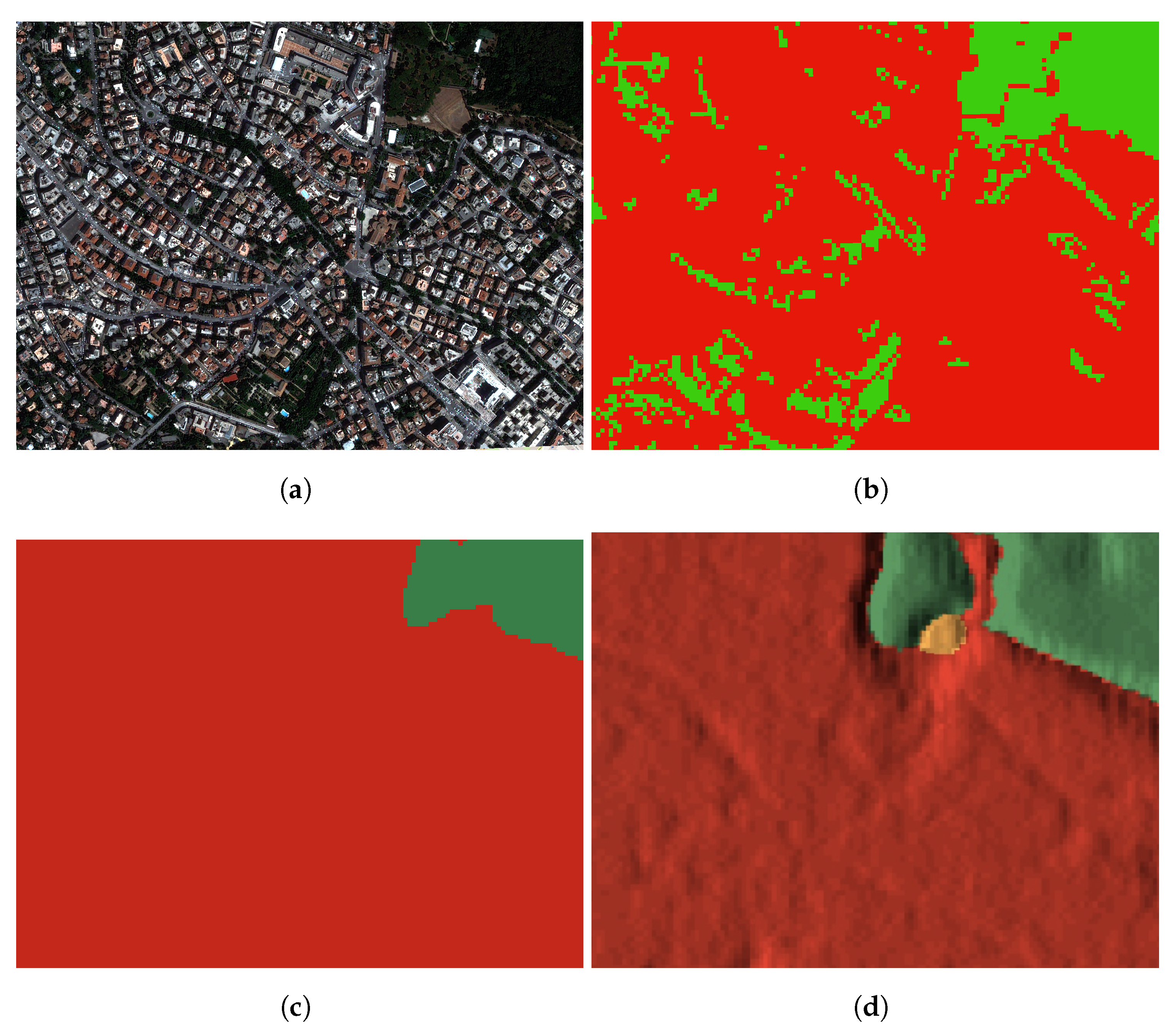To better understand the extent of this problem in urban areas, in Figure 1 we compare different imperviousness maps for the same land portion covering a small area in the city centre of Rome, Italy. 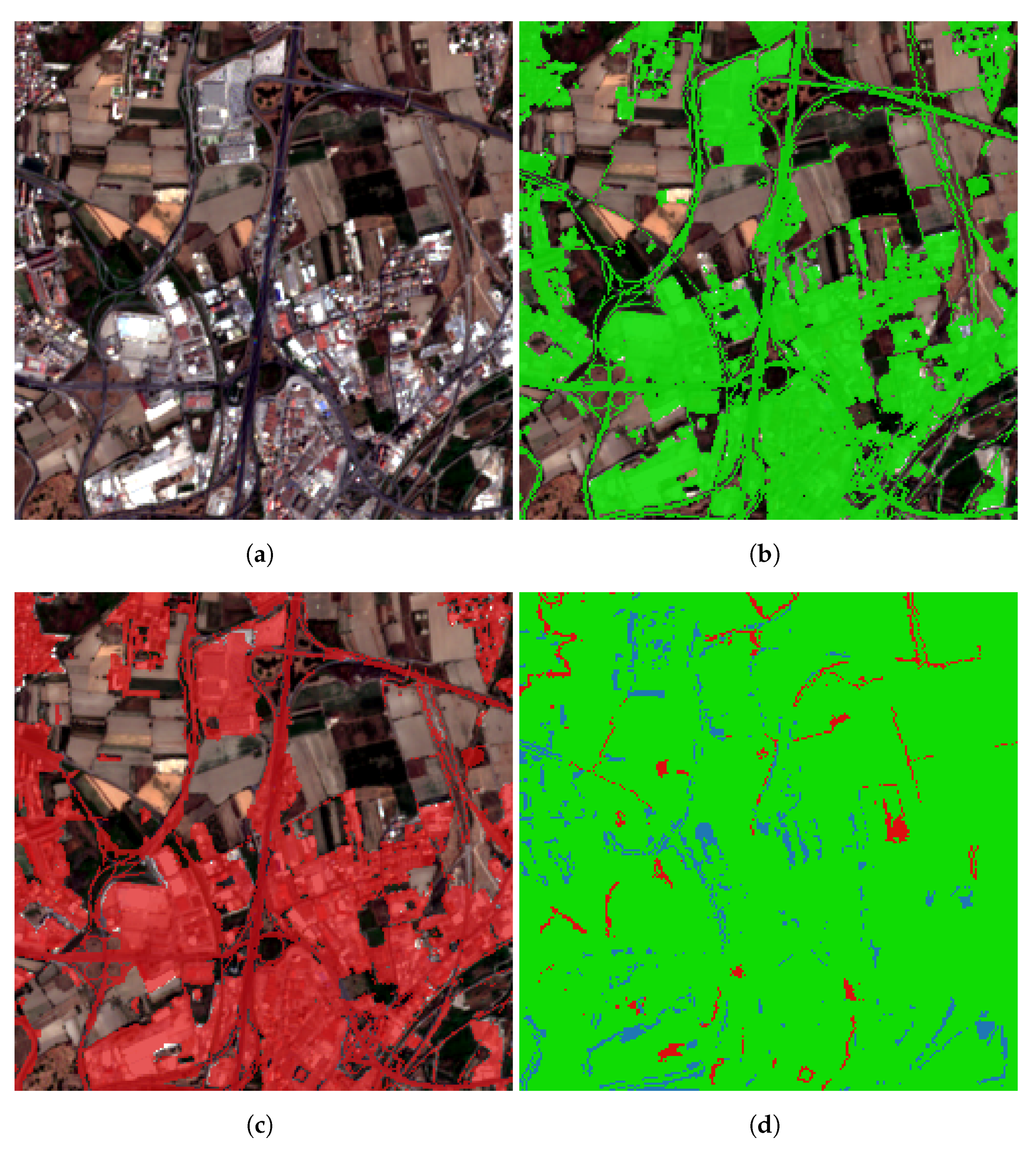In particular, Figure 1a shows the area as it appears from very high-resolution (50 cm) Pleiades satellite image; Figure 1b shows the imperviousness map at 10 m resolution realised by on-plane analysis performed by the Italian National Institute for Environmental Protection and Research (ISPRA (https://www.isprambiente.gov.it/)); Figure 1c reports a 10 m imperviousness map realised by the Environmental Systems Research Institute (ESRI) using artificial intelligence algorithms; finally, Figure 1d shows a 10 m imperviousness map currently available on the Google Earth Engine under the name of “DynamicWorld”, automatically generated using deep learning on Sentinel-2 imagery [6].

Furthermore, recent years have seen an enormous increase in the number of web-based applications leveraging techniques derived from geographic information systems (GIS). Even though it should be good news to have access to spatial data as well as advanced mapping and spatial analysis over the Internet as a critical point to pursue reduction of the distance between data, information and decision-makers, it has often been observed that many publicly available map layers are actually only accessible by people skilled with GIS. In this work, we want to tackle these problems by assembling a novel dataset, experimenting with a DL architecture designed to take advantage of Sentinel-2 multi-spectral data, and integrating the whole process in a proof-of-concept web application. In particular, the main contributions of this work can be summarised as follows:

• To address the difficulties of the current solutions in the urban context, a new dataset has been gathered using an authoritative imperviousness map (ISPRA) as ground truth. ISPRA is a public institute, part of the Italian Ministry for the Environment, Territory and Sea, promoting and supporting scientific, technical and research functions as well as assessment, monitoring and control activities. Among other functions, it provides several land-cover maps, including the imperviousness map used in this work. These maps are produced semi-automatically from data provided by several European projects and authoritative data available for Italian territory, and are generated and released yearly;
• We introduce ReFuse, a new DL architecture for impervious surface extraction based on a U-Net backbone [7], residual blocks (Re) [8] and the FuseNet principle (Fuse) [9] to take advantage of Sentinel-2 multi-spectral bands despite their different spatial resolutions. We also compared the performance of the proposed approach against some state-of-the-art CNNs;
• We integrated imperviousness inference and visualization into a GIS web application with a user-friendly interface for users without specific GIS competencies, implementing an inference pipeline leveraging modern distributed parallel computing and MLOPs best practices. This enables fast deployment of the solution on HPC or cloud computing systems, ensuring high scalability.

The rest of the paper is structured as follows: Section 2 reports some related works; the process of the dataset generation, the proposed DL approach for impervious surface extraction and the web tool are described in Section 3; Section 4 describes the experimental setup; Section 5 reports and analyses obtained results while Section 6 provides some conclusions and future perspectives.

2. Related Works

Computer vision and machine learning strongly contribute to satellite image classification. Focusing on remote-sensing methods for impervious surface extraction, machine-learning approaches can be divided into three groups: (i) pixel-based, (ii) texture-based and (iii) semantic segmentation algorithms [10].

Pixel-wise classifiers typically exploit the spectral signature by relying on ad hoc features. Usually, they leverage a similarity measure to measure the spectral differences between impervious surfaces and other ground objects. Most commonly used indexes are Normalised Difference Built-up Index (NDBI) [11,12], Normalised Difference Vegetation Index (NDVI) [11,13], Index-based Built-up Index (IBI) [14], Normalised Impervious Surface Index (NISI) [15], Combination establishment index (CBI) [16] and Corrected Normalised Difference Impervious Surface Index (MNDISI) [17]. These methods are usually computationally not demanding. The flip side is that pixel-based approaches ignore spatial context information. This implies that they can easily be misled by the noise and the within-class variability, causing a salt-and-pepper effect within the classification result. Instead, the texture-based approaches do not rely on the spectral information of imagery but rather exploit spatial information among neighbouring pixels to overcome the noise better and to capture different types of spatial structures. Given a set of features to take into account, different classification methods have been used to divide pixels into impervious and permeable surfaces. Commonly used classifiers include Support Vector Machines [18,19], artificial neural networks [20], decision trees [21] and random forest [22].

The wide variety of solutions so far described highlights the difficulty in finding the best combination of features that suit the classification task due to the high variability of impervious surfaces’ appearance on remote-sensing imagery [1]. Therefore, this task can benefit from data-driven feature-learning approaches and end-to-end model training provided by semantic segmentation algorithms [23]. In the past decade, deep learning has proved to be effective on this task, with Convolutional Neural Networks (CNN) outperforming many traditional machine-learning solutions. Nearly all state-of-the-art architectures for semantic segmentation follow principles stated in [24], where semantic segmentation using Fully Convolutional Networks (FCN) are demonstrated to be able to achieve impressive results. The main idea consists of modifying traditional CNN so that the output is no longer a probability vector but rather a probability map. That was possible by replacing standard fully connected layers of CNNs with fully convolutional layers to “densify” the single-vector output of a traditional CNN. A second feature was the use of transposed convolutions, also called deconvolutions. A deconvolution layer is used for up-sampling a feature map and obtaining a prediction of the same size as the input image [25]. The third feature was the skip connections to combine dense prediction at shallow layers and coarse predictions at deep layers, improving segmentation details.

On this line, several architectures have been so far proposed. The U-Net architecture [7], designed for biomedical image segmentation, introduced the encoder–decoder paradigm for up-sampling gradually from lower-size features to the original image size. Since then, almost all CNN models for semantic segmentation have some form of encoder–decoder structure. The encoder reduces the spatial resolution of the input and creates lower-resolution feature mappings that are highly effective at classifying objects. The decoder increases the resolution of the feature representations to create a full-resolution segmentation map. U-Net added several skip connections, which concatenates the feature maps of the encoder part with the mirrored feature maps in the contracting path.

In [26], Sun et al. experimented with the use of a CNN to extract impervious surfaces through Worldview-2 and airborne LiDAR. The findings showed that 3D-CNN had more ability to extract features than SVM since it used pixel-level spatial information as well as texture. Ref. [27] uses a deep-learning approach to extract impervious surfaces from WorldView 2 and Pléiades-1A datasets automatically. In [28], the authors conducted a comparative study for the impervious surface estimation mixing optical and SAR data; experimental results indicated the effectiveness of the proposed deep convolutional network, which exhibited a better accuracy outperforming other benchmark methods. In [29], Fu et al. proposed a solution based on a deep CNN to map impervious surfaces in town–rural areas using China’s GF-2 Imagery. They showed the effectiveness of deep models and how transfer learning could significantly boost overall accuracy.

Fewer studies are available on using Sentinel-2 imagery for built-up ISA extraction and even less with a deep-learning approach. In [30] the authors assessed the feasibility of using Sentinel-2 images for this task by means of an artificial neural network. In [31], using Sentinel-2 satellite imagery, a CNN was employed as a deep feature extractor, and the classification was made by means of a random forest classifier. Similarly, in [32] the authors compared different machine-learning and deep-learning algorithms for the land-cover classification, with a CNN showing the best performance in the classification of impervious areas. Deep learning has also been investigated for multi-sensor and multi-modal image segmentation. Multi-modal fusion strategies are of great interest in the field of RS classification since satellite images usually consist of multi-spectral content. Similarly, extensive research has also been conducted to combine heterogeneous data (multi-sensor fusion), such as optical images with Synthetic Aperture Radar (SAR) and LiDAR data. In both cases, fusion models help reduce confusion from spectral heterogeneity in landscapes and enhance classification accuracy. On this line, in [33] the authors use existing CNNs (FCN or SegNet) as a base network to experiment with different data fusion strategies, both in early and late fusion fashion. In the same way, Ref. [34] explores how deep fully convolutional networks can be modified to handle multi-modal and multi-scale remote-sensing data for semantic labelling. To this aim, the authors extended the FuseNet architecture [9] by considering two branches, one trained with IR-R-G bands and one with Normalised Digital Surface Model (NDSM), Digital Surface Model (DSM) and NDVI data. The proposed approaches outperformed a SegNet trained only on IR-R-G bands, thus proving the effectiveness of using multi-spectral data for remote-sensing classification.

3. Materials and Methods

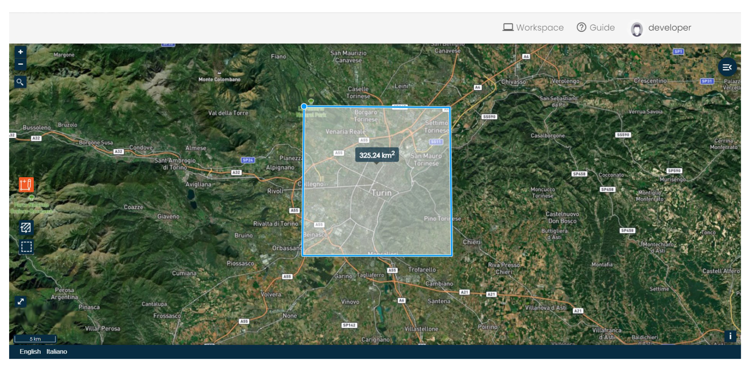
As described in Section 1, in this paper we introduce a web-based system leveraging a new deep-learning model for generating imperviousness maps from Sentinel-2 satellite images. The resulting system has been integrated within a GIS web-based application to support non-expert operators in easily generating imperviousness maps. Figure 2 shows the interface presented to the user for requesting a map of imperviousness in a specific part of the globe. Users only need to draw their area of interest and then select the date range in which they are interested. Once the area and date range has been selected, a map calculation phase for the specific area starts. An asynchronous process handles the whole computation. All these processes happen in the background and are transparent to the user. Figure 3 reports a logical diagram of the inference pipeline: after the user request, satellite images are collected from the stores and sent to the inference pipeline, which produces the imperviousness map as the final output. It is worth noting that such a web application requires an inference process that can handle and scale toward enormous quantities of satellite data. The following sections detail each of the three main components: Section 3.1 describes the steps followed for the training dataset generation; Section 3.2 introduces the designed deep-learning model; Finally, Section 3.3 describes the inference pipeline in detail, investigating the scalability requirements of the proposed solution.

3.1. Imperviousness Dataset Generation

This section describes the methodology we used to create the dataset to be used to train our deep-learning model for generating imperviousness maps from Sentinel-2 satellite images (dataset openly available in Zenodo at https://doi.org/10.5281/zenodo.7058860 accessed on 22 September 2022). The Sentinel-2 platform consists of two satellites equipped with sensors able to acquire images with 13 spectral bands ranging from the visible range to the short-wave infrared. Each sensor has a different spatial resolution, with RGB bands and near-infrared (NIR) showing the highest one (i.e., 10 m). With a 12-bit radiometric resolution, the image can be collected from 0 to 4095 possible light intensity values, enabling the satisfactory identification of minor variations in reflected or emitted energy.

The lack of labelled data poses a serious obstacle to developing deep-learning algorithms that detect impermeable surfaces. Most available imperviousness maps typically have a coarse spatial resolution that does not adequately emphasize green spaces in urban settings. In this work, we used the soil consumption map covering Italy provided by ISPRA for 2017 with a 10 m spatial resolution. These data were built by merging regional Land Use Land Cover (LULC) maps, in situ data provided to ISPRA by Regional Environmental Agencies, Copernicus HRL Imperviousness products, OpenStreetMap, and local supplementary data. The map consists of a hierarchical classification ID with each pixel having up to three digits class: the first digit, starting from the left, describes whether a point is consumed soil (i.e., a value of 1) or not consumed soil (i.e., a value of 2), while the other two optional digits can specify the class with more detail (e.g., 112 stands for “soil consumed by asphalt roads”). Since we were interested in the segmentation between impervious and non-impervious surfaces, only the first digit was considered to label the data.

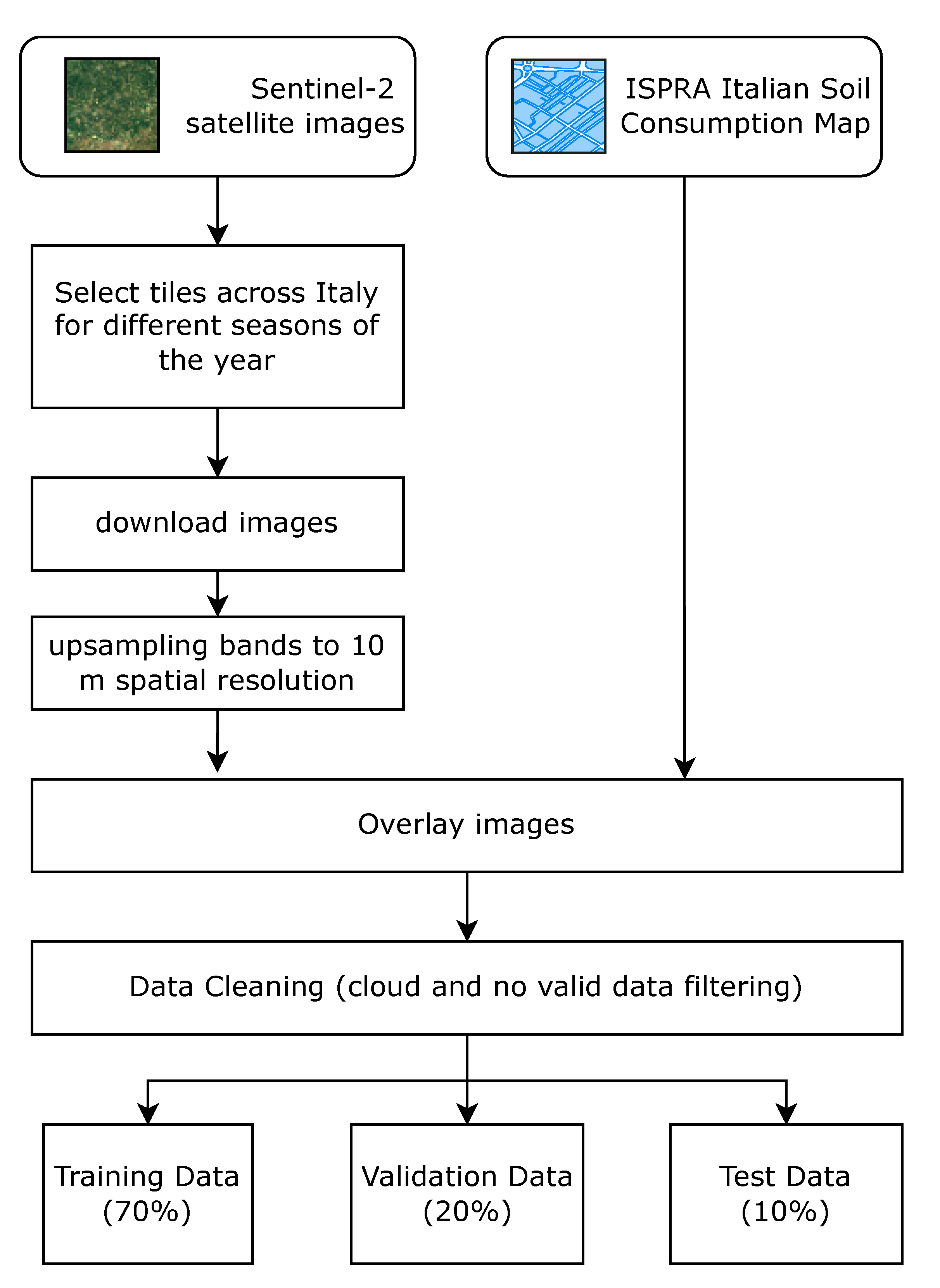
The flowchart in Figure 4 illustrates the process used in this work for generating labelled training, evaluation, and testing data. Sentinel-2 granules are organized in a tiling, partially overlapping grid. As for other image-processing domains, having a dataset representative of the population is crucial. As the authors of this paper are Italian, we decided to select Sentinel-2 tiles covering particular zones of the Italian peninsula containing a variegate distribution of hills, waters, plains, mountains, etc., both in urban and suburban realms. To further increase the variance, we extracted images recorded all over the year, acquiring at least one image per season. Nonetheless, it is worth noting that only images for 2017 were considered, to minimize labelling mismatch with the available ground truth.

Table 1. List of Sentinel-2 products used for the generation of the dataset.

Month	Product Name Identifier
March	S2A_MSIL2A_20170329T095021_N0204_R079_T33TVF_20170329T095024
June	S2A_MSIL2A_20170613T101031_N0205_R022_T32TQR_20170613T101608
July	S2A_MSIL2A_20170720T100031_N0205_R122_T33TUH_20170720T100027
July	S2A_MSIL2A_20170706T102021_N0205_R065_T32TMQ_20170706T102301
August	S2A_MSIL2A_20170806T095031_N0205_R079_T33TWF_20170806T095744
August	S2A_MSIL2A_20170802T101031_N0205_R022_T32TQP_20170802T101051
October	S2A_MSIL2A_20171014T102021_N0205_R065_T32TNR_20171014T102235
October	S2A_MSIL2A_20171015T095031_N0205_R079_T33SVB_20171015T095944
October	S2A_MSIL2A_20171028T100121_N0206_R122_T33TUG_20171028T134729
December	S2A_MSIL2A_20171220T101431_N0206_R022_T32TPR_20171220T122057
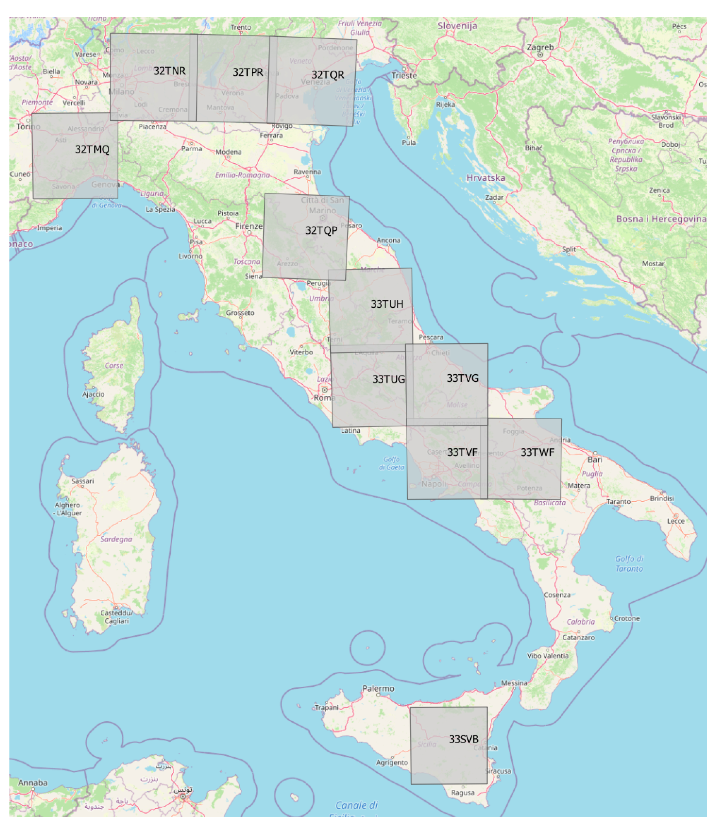
December	S2A_MSIL2A_20171224T095421_N0206_R079_T33TVG_20171224T122256

lists Sentinel-2 products used for the dataset generation while Figure 5 shows selected patches distribution along the Italian peninsula.

Sentinel-2 bands with lower spatial resolution were up-sampled to 10 m per pixel using cubic convolution. When necessary, ground-truth raster and acquired Sentinel-2 images have also been reprojected to a common coordinate system to have two perfectly stackable files. It is worth noting that a typical Sentinel-2 tile has a size of 10,980 × 10,980 pixels for the 10 m spatial resolution. Since these dimensions are computationally infeasible, we extracted non-overlapping patches of $244\times 244$ pixels from each ground-truth image. Finally, a data-cleaning process excludes chips without corresponding ground truth, i.e., chips containing no data values or chips with clouds. To this aim, a cloud mask is computed using the Scene Classification Layer within Sentinel-2 Level-2A products.

3.2. Multi-Spectral Bands Fusion Network

Semantic labelling of satellite images requires a dense pixel-wise image classification. In this work, we started exploring some popular neural networks’ capabilities for pixel-wise extraction of impervious surfaces. However, it is crucial to consider that Remote-Sensing (RS) image data are more than a picture since they include electromagnetic wavelengths ranging beyond the three RGB bands of natural images. In general, a CNN can take an arbitrary number of spectral bands as input, modifying the depth of the first input convolutional layer. However, exploiting the multi-spectral content of RS images is not as simple as presenting more bands as input to the network. Indeed, increasing the number of spectral input bands eventually results in the need for more extensive training datasets, consisting of satellite images and corresponding ground-truth data, to avoid incurring in overfitting. Moreover, this approach does not allow for leveraging transfer learning, which instead proved to be effective for remote-sensing image analysis [35]. In a multi-sensor setup, with more than three bands available, a possible approach is to employ two or more neural network branches to analyse some of the bands separately, fusing the features at a later stage in the network. However, the main drawback of this late fusion procedure is that the number of weights doubles, thus requiring more computation time for both the training and inference phase. Considering the extension of satellite images, this limitation might be too demanding to make the approach feasible in a real production environment.

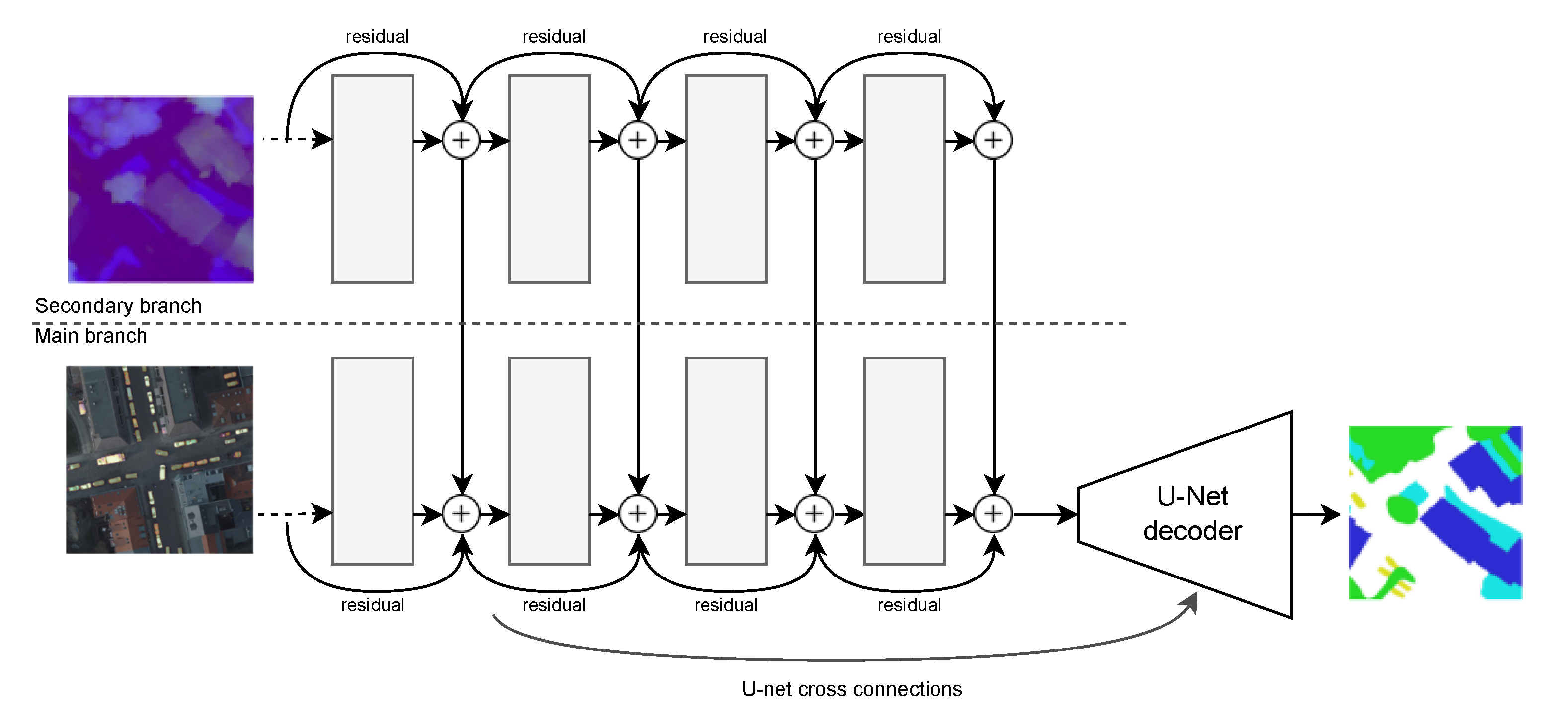
In this paper, we thus focus on designing a CNN able to efficiently combine features from multi-spectral bands, providing a good balance between the number of parameters and segmentation performance. The proposed architecture, shown in Figure 6, comprises three state-of-the-art ideas:

• A U-Net as backbone architecture. Its encoder–decoder paradigm with cross-connections for pixel-wise labelling and skip connections between same-sized parts in down-sampling\ up-sampling paths help to address the loss of fine detail during up-sampling [7];
• To achieve better results as the depth of the network increases, the building blocks of the standard U-Net encoder part were replaced with residual blocks. More in detail, a ResNet-50 model has been used to replace the U-Net encoder down-sampling section. The idea is to leverage residual blocks’ ability to reduce the problems associated with the vanishing gradients strongly;
• To exploits multi-spectral content, beyond classic RGB wavelengths, a FuseNet [9] approach has been used. The FuseNet model jointly encodes both the RGB and depth information using two encoders (in this case, two ResNet-50, as described in the previous point) whose contributions are summed after each convolutional block. We adapted the standard fusion approach to the use of residual networks by summing contributions from different branches after each residual block.

The result is a U-Net-like network with the encoder replaced by two parallel ResNet-50 networks where the main branch inputs the RGB bands while the second uses bands B07, B08, and B11. Every residual block output from the second branch is fused into the main branch by employing feature map summation. After that, the fused map is connected to a convolutional layer for the decoding part through concatenation, implementing the classical U-Net cross-connections. All these solutions allow the proposed architecture to benefit from the combination of short (i.e., residual skip connections) and long skip connection (i.e., U-Net cross-connections) during the training strategy. We named this approach ReFuse after its two core components: REsidual blocks and FuseNet.

Some minor changes were applied to the ResNet-50 encoder, following the minor adjustments presented in [36]. At first, we modified the down-sampling block of a ResNet-50, changing the stride of the first convolutional layer from 2 to 1. The idea behind this is that a stride of 2 with a kernel size 1 × 1 ignores three quarters of the input feature map. To leave unchanged the spatial size, we switched the size of the strides in the first two convolutions, so that the second convolutional layer will have a stride of 2. Second, for the same reasons, we replaced a 2-stride convolution with an average pooling layer followed by a 1 stride convolution, keeping intact the output dimensions: adding a 2 × 2 average pooling layer with a stride of 2 before the convolution 1 × 1 with a stride of 1 the model will not overlook any information. Finally, we changed the first convolutional layer of the ResNet (i.e., a 7 × 7 convolution) with three 3x3 convolutions, since the replacement will make the model easier to train [36].

Finally, to leverage transfer learning, we adopted a three-step training approach: (i) the encoder weights are initialized from a ResNet50 pre-trained on ImageNet; (ii) the training is started with all the encoder layers frozen (with the aim of training only the decoder ones); (iii) the network is trained again by considering all the layers trainable. This procedure helps the network to converge while giving the decoder enough information to learn how to produce helpful segmentation masks properly.

3.3. Distributed Inference Pipeline

Serving a model in production is crucial, especially when we need to serve a web-based application. Once the model is trained, we need to deploy it in a way that it can serve the application. Building highly available, scalable, distributed systems for machine-learning data pipelines is a complex task. In this work, we managed the whole process as a workflow, a sequence of tasks representing units of business logic. Figure 7 shows the workflow implemented for the prediction pipeline. The workflow is a Directed Cyclic Graph (DAG) where each node is a task and arrows are dependencies between tasks. In the extraction step, from the AoI and date range provided by the user, a first task searches and downloads Sentinel-2 data. Any images with clouds are appropriately removed from the process. The prediction is performed on the downloaded images after a subdivision into patches of the size required by the deep-learning model. Finally, merging predicted patches, the map is assembled and stored for later visualization.

We implemented the whole approach through a Workflow Management System (WfMS) (Source code is available at https://github.com/priamus-lab/ReFuse accessed on 22 September 2022). A WfMS provides an infrastructure for a defined workflow’s setup, performance and monitoring. Therefore, involving a WfMS gives flexibility and extendibility to the approach because it implements off-the-shelf features such as data-sharing between tasks, recovery from failure, retrying failed tasks, task scheduling for batch runs, flow versioning and more. In this study, we use Prefect (https://www.prefect.io/ accessed on 31 July 2022), an open-source orchestration and workflow tool. However, despite the choice made, this work aims to show a general approach, easily replicable with similar tools. We can highlight five essential layers in every WfMS (Figure 8): (i) the orchestration layer, which is responsible for the workflow’s life cycle; (ii) the agents, daemon-like processes that look for tasks and run them if any are available; (iii) the flow run layer, which is responsible for defining where the flow run; (iv) the execution layer, which manages where and how single tasks within the flow run; (v) the storage layer, which defines where the flow’s code is stored, to be collected when needed. In addition, when tasks need to pass data between them, we need a result layer which defines and manages where to store task results.

It is worth pointing out that in a fully distributed system such as the one we are defining, the layers and components can be chosen from different types and deployed in different places. This aspect makes the solution extremely flexible: for example, in a development and test phase, one could choose to deploy an agent on a personal computer but let the flow run in the cloud. Figure 8 highlights in bold choices made in this work. Both agents and flows ran on a Kubernetes cluster; Prefect Cloud, a cloud-managed service, performed the orchestration. Flow’s code and task results were stored in an object-based storage, in particular an AWS S3 bucket. Kubernetes is a system that manages containers where a container could be explained as a lightweight virtual machine. Containers encapsulate an application with all its dependencies, including system libraries, binaries, and configuration files, making it portable across different hosts. Kubernetes can create and scale these containerized applications automatically and manage storage among all the containers. Instead, object-based storage is a strategy that manages and manipulates data storage as distinct units called objects. Data are kept in separate storehouses versus files in folders and is bundled with associated metadata and a unique identifier to form a storage pool. Object-based storage effectively manages unstructured distributed content such as our use case. This solution is adaptable to different scenarios because the business logic is separate from the execution methods. Changing the configuration of one of the components, e.g., where to store the code or execute the flow, does not require any change to the business logic of the tasks. We choose to use a Dask cluster for the execution layer. This is the most critical choice in our pipeline, as the choice of this executor allowed us to parallelise task execution and potentially scale the approach indefinitely in a distributed environment. Dask is an open-source Python library for parallel computing. In particular, we created an ephemeral Dask cluster, i.e., a cluster that scales up and down when needed and executed tasks on them. Despite an initial latency time to start up the cluster, an ephemeral cluster allows the leveraging of several machines but releasing them when the workload completes. The WfMS was in charge of orchestrating all the tasks together, respecting dependencies and data flow between them. Figure 7 highlights parallelisable computations within the inference pipeline. It shows with green arrows the outputs of tasks that produce a list of elements on which subsequent tasks can proceed in parallel. The designed workflow involves parallelisation in processing the identified Sentinel-2 images and inferring over the patches into which the image is divided. For example, if the initial search step identifies 100 Sentinel-2 images, subsequent processing can proceed in parallel on these. A workflow such as this can be optimized with a map-reduce approach. Map-reduce is a powerful two-stage programming paradigm, very famous in the big-data ecosystem, that can be used to distribute and parallelise work (the “map” phase) before collecting and processing all the results (the “reduce” phase). We can execute tasks dynamically across an iteratable input with a map-reduce model. This, in turn, allows us to execute mapped tasks in a distributed and parallel manner on a Dask cluster, drastically reducing the total execution time.

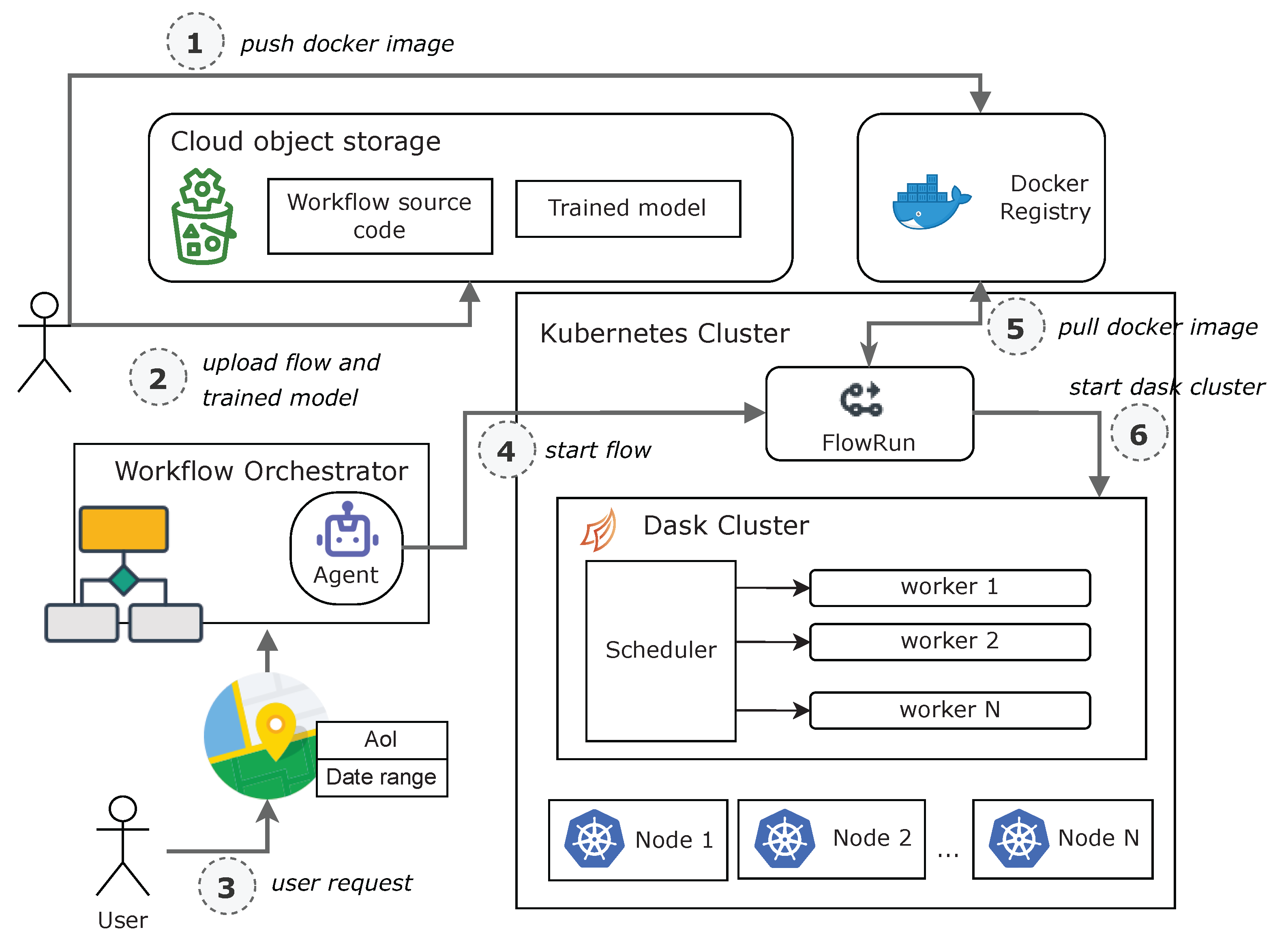
Figure 9 depicts the whole process. The first step is releasing the Docker image for the flow execution into a Docker registry. A Docker image is an immutable template file containing the source code, libraries, dependencies, tools, and other files needed to create a container where the application will run. In this way, we are sure that nodes which execute the inference pipeline will have all software dependencies correctly in place. The model-serving strategy adopted is straightforward: together with weights, the model was stored in object-based storage. This method permits the download of the model for inference using a URL accessible via the Internet, a mandatory requirement for a distributed data pipeline. In addition, it enables a fast and easy replacement with newer versions because the model and business logic are decoupled. Finally, these steps can easily be automatized within a Continuous Deployment flow, e.g., by initiating automatic uploads following a code committed into a code repository. At the user’s request to calculate the imperviousness map on a new area, a request is sent for a new execution of the inference flow. The agent, therefore, upon receiving the request, starts the flow. The flow is executed within a Kubernetes cluster in the form of a Kubernetes job. A Kubernetes job is a workload controller that performs one or more finite tasks in the cluster. At startup, the flow pulls the Docker image from the Docker registry for machine instantiation and then deploys an ephemeral Dask cluster. After the Dask cluster is up, flow tasks can execute appropriately on the cluster. A Dask cluster is composed of one scheduler node and N worker nodes. By increasing the number of workers, we can scale up the number of maximum tasks executable in parallel, giving our solution great flexibility and scalability. Although not mandatory, such a solution fits well with the serverless infrastructure made available by most cloud providers today. Serverless computing is an execution model in which the cloud provider allocates machine resources on demand, allowing customers to pay only when computational power is needed. Creating a Dask cluster when required and deploying it on a serverless infrastructure dramatically reduces operational costs while maintaining a virtually infinite ability to scale. It is worth remarking that the type of machine used to instantiate Dask workers can be defined during configuration. For example, machines with GPU enabled can be selected to reduce inference time further.

4. Experimental Setup

We implemented the network in PyTorch, and the training execution was on ad hoc AWS EC2 instances. We trained all our models using the Adam optimizer [37] with ${\beta }_1=0.9$, ${\beta }_2=0.99$, $ϵ=1^{-5}$, a weight decay of $1^{-2}$ and a batch size of 8. The considered loss function is a combination of dice and pixel-wise cross-entropy loss:

$$L_{total}=L_{dice}+L_{ce}$$

with

$$L_{ce}=-(ylog\left(p\right)+(1-y)log(1-p))$$

$$L_{dice}=1-\frac{2\left|A\cap B\right|}{\left|A\right|+\left|B\right|}$$

where A is the predicted segmentation mask and B is the ground truth, y is the ground truth, and p is the probability for that class. The choice of also including the dice loss is to help to regularise results in the case of unbalanced data chips (e.g., $95\%$ bare soil and $5\%$ impervious surface in a single chip).

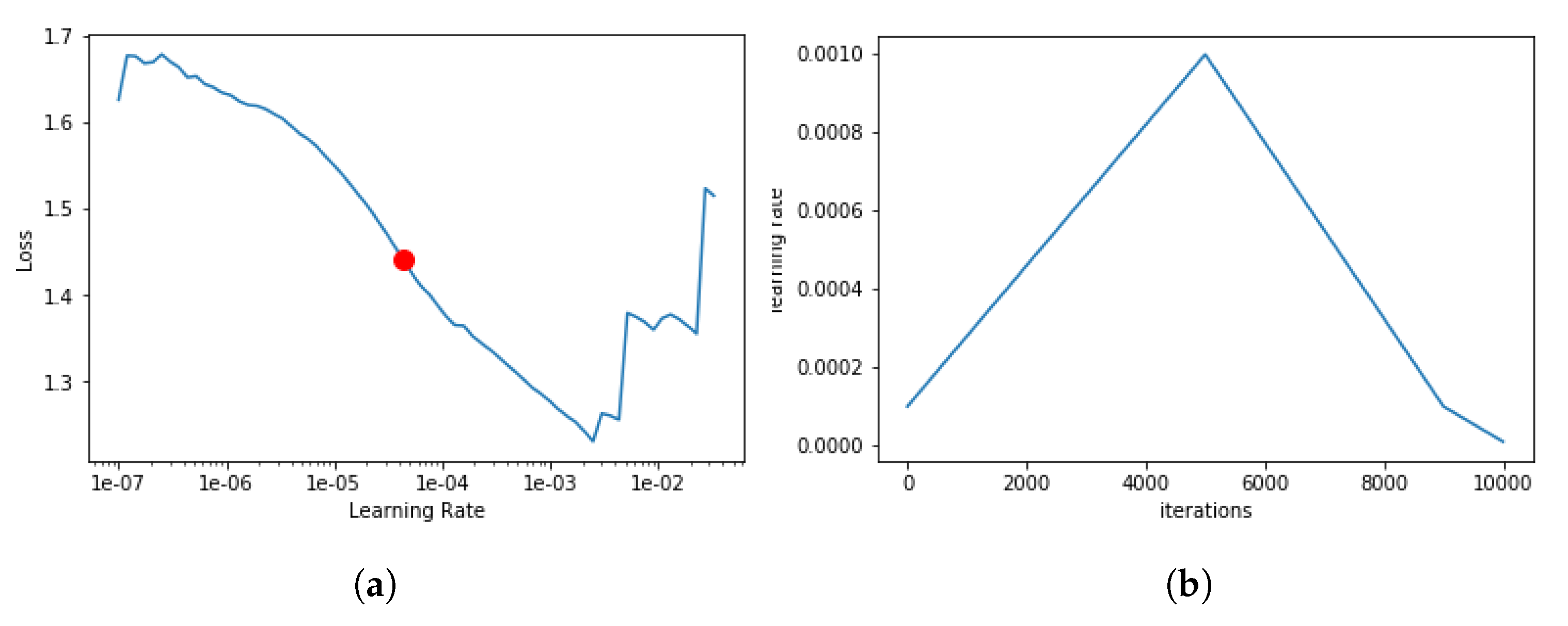
One of the most critical hyperparameters is the learning rate (LR): a big LR causes the model to diverge, while a small LR causes the model to converge slowly or stack in an unfavourable solution. We used two methods, the learning rate range test [38] and the one-cycle policy [39], to determine the ideal LR value and train the model for accurate fine-tuning. The LR range test is a method for determining what are considered to be the acceptable minimum and maximum boundary values for LR. It entails running the model over several epochs while letting the LR rise linearly between low and high LR values after each mini-batch until the loss value increases enormously. Plotting accuracy trend variating LR values, we can choose the LR one order lower than the point where loss is minimum. Figure 10a shows the output for ReFuse model learning range test: we chose a maximum LR of $1^{-3}$. On the other hand, one-cycle policy is a technique similar to the simulated annealing algorithm [40] designed for varying the LR during the training. The method needs an initial interval of values: we choose the maximum value using the LR range test and the lower one as 1/10th of the maximum LR. The algorithm moves from the lower to the higher value during the first half of the cycle and from the higher back to the lower during the latter half of the cycle. Finally, in the last few iterations, this method anneals the learning rate way below the lower learning rate value for a final fine-tuning. Conventionally, the learning rate decreases as the learning start converges, but the idea behind this approach is that a higher learning rate may help overcome saddle points. In [39] the author shows that when the learning rate is higher, during the middle of learning, the learning rate works as a regularisation method and keeps the network from overfitting because it avoids steep areas of loss and finds a better flatter minimum. Figure 10b shows LR values used during training across the considered iterations. As soon as the model performance on the validation dataset ceased improving, we employed an early-stopping criterion to stop the training.

The GIS web application and the inference pipeline were executed on cloud infrastructure, using a Kubernetes cluster. In particular, the inference pipeline was released on a serverless infrastructure to reduce the solution’s running costs.

5. Results

We compared our solution against some state-of-the-art CNNs and variants to measure the effectiveness of the proposed approach. In particular, we compared against some variants of three main architectures:

• We trained an FCN-8s, a variant of an FCN model introduced in Section 2. The classical FCN architecture consists of a series of convolutional and pooling layers, with FCN-8s also implementing a fusing strategy between predictions of the shallower layer Pool3 with twice-up-sampled sum of the two predictions derived from Pool4 and the last layer. The stride 8 predictions are subsequently up-sampled back to the image;
• We investigated the use of a standard U-Net using different pre-trained CNNs as encoders. In particular, we explored the use of VGG16 [41], ResNet [8] and EfficientNet [42] architectures pre-trained on ImageNet. The reasons behind this choice are the high generalization ability demonstrated over the years by VGG, the ability to deal with gradient vanishing of ResNet and the high efficiency/performance trade-off of EfficientNet;
• We used also DeepLabv3+ [43], an architecture introducing changes to the encoder–decoder structure, such as the use of dilated convolutions [44], to preserve most of the spatial input information.

We tested these architectures with different bands as input (i.e., RGB, RGB + NIR, all 13 bands resized to have the same spatial resolution). In all the experiments, as evaluation metrics, we used the pixel-wise segmentation accuracy and the Intersection over Union (IoU), defined as:

$$IoU=|Predicted\cap GT|/|Predicted\cup GT|$$

where $GT$ is the ground-truth imperviousness mask. Table 2 reports the results for the considered analysis, reporting for each configuration the base architecture, the used encoder (if any), the used input bands and the obtained performance. The table clearly shows that the proposed approach outperforms all the considered competitors by a large margin. Moreover, analysing the table, there are a few points worth highlighting:

• Models trained on RGB bands and using transfer learning (with weights pre-trained on ImageNet) tend to perform better than those using a different combination for the bands;
• Results obtained using all bands at 10 m spatial resolution, i.e., RGB and NIR, are slightly comparable with results obtained with RGB bands only;
• ResNet-50 tends to be the most effective encoder;
• Using all 13 bands causes the worst results both in terms of accuracy and IoU. This confirms our claim that using more bands does not necessarily result in better performance.

Table 2. Results obtained by the proposed approach (last row) and the considered competitors for the imperviousness map extraction. For the proposed approach (ReFuse), the use of brackets under the “bands” column highlights the ability of the proposed approach to use different bands type, without the need for resizing.

Network	Encoder	Bands	Accuracy	IoU
FCN-8s	-	R, G, B	89.54%	69.76%
FCN-8s	-	R, G, B, NIR	88.25%	69.55%
FCN-8s	-	All 13 bands	84.80%	60.35%
U-Net	VGG16	R, G, B	87.45%	70.03%
U-Net	ResNet-34	R, G, B	90.13%	70.54%
U-Net	ResNet-50	R, G, B	92.39%	73.50%
U-Net	ResNet-50	R, G, B, NIR	92.07%	71.37%
U-Net	ResNet-50	All 13 bands	89.37%	70.32%
U-Net	ResNet-101	R, G, B	90.39%	70.57%
U-Net	EfficientNetB7	R, G, B	94.48%	74.61%
DeepLabv3+	ResNet-50	R, G, B	92.19%	71.35%
DeepLabv3+	ResNet-50	R, G, B, NIR	91.32%	71.29%
DeepLabv3+	ResNet-50	All 13 bands	88.25%	68.50%
ReFuse	ResNet-50	(R, G, B) + (B7, B8, B11)	95.72%	75.85%

Table 2. Results obtained by the proposed approach (last row) and the considered competitors for the imperviousness map extraction. For the proposed approach (ReFuse), the use of brackets under the “bands” column highlights the ability of the proposed approach to use different bands type, without the need for resizing.

Network	Encoder	Bands	Accuracy	IoU
FCN-8s	-	R, G, B	89.54%	69.76%
FCN-8s	-	R, G, B, NIR	88.25%	69.55%
FCN-8s	-	All 13 bands	84.80%	60.35%
U-Net	VGG16	R, G, B	87.45%	70.03%
U-Net	ResNet-34	R, G, B	90.13%	70.54%
U-Net	ResNet-50	R, G, B	92.39%	73.50%
U-Net	ResNet-50	R, G, B, NIR	92.07%	71.37%
U-Net	ResNet-50	All 13 bands	89.37%	70.32%
U-Net	ResNet-101	R, G, B	90.39%	70.57%
U-Net	EfficientNetB7	R, G, B	94.48%	74.61%
DeepLabv3+	ResNet-50	R, G, B	92.19%	71.35%
DeepLabv3+	ResNet-50	R, G, B, NIR	91.32%	71.29%
DeepLabv3+	ResNet-50	All 13 bands	88.25%	68.50%
ReFuse	ResNet-50	(R, G, B) + (B7, B8, B11)	95.72%	75.85%

To better understand the effectiveness of the proposed approach, in Figure 11 we report an inference example on a single patch, highlighting false positives (FP) and false negatives (FN). Interestingly, ReFuse produces a segmentation mask very close to the ground truth, with errors almost all located along the borders of the urban areas or in shadow zones (misclassified as impervious areas). Similarly, Figure 12 reports the extraction results from the test set of two representative regions in the city of Turin in Italy, including small dense residential buildings and large high buildings in urban commercial areas. For both areas, the model produces excellent segmentation masks. Both images in Figure 12d,h reveal some difficulty in segmenting small buildings and noise along the edges of streets. This result can be explained in the first instance by the spatial resolution of the Sentinel-2 data. A spatial resolution of 10 m is too low to capture such levels of detail. Indeed, even observing Sentinel-2 images (Figure 12b–f) by the naked eye, we can exhibit the same difficulty in discriminating between impervious and non-impervious pixels.

It is worth noting, finally, the presence of mislabelled data shown in Figure 12c. Despite the presence of trees and gardens, everything is labelled as impervious. Even more interesting here is the result obtained. Despite errors in the ground truth, the network correctly detects the green infrastructure within the area, i.e., trees, grass and parks, showing an ability to generalize the result that is sometimes superior to that of the training data. This result is of fundamental interest in this work because, as stated in Section 1, one of the objectives was to address the difficulties of current solutions in extracting imperviousness maps with a high level of detail within the urban context.

6. Conclusions

In this study, we introduced a deep-learning-based method for extracting imperviousness maps from multi-spectral Sentinel-2 pictures leveraging bands with different spatial resolutions without the need for rescaling or other adaptations. Additionally, the proposed approach has also been made available through a portable and scalable inference pipeline, easily pluggable within a web-based GIS application. The aim is to support the generation of imperviousness maps as soon as new satellite images are available for a fast, effective and reliable analysis of human environmental impact. To achieve this, one of the biggest challenges was the lack of a labelled dataset, with a temporal and spatial granularity, as well as precision, suited for the task. To address this problem, we gathered a new dataset using the ISPRA imperviousness map as the ground-truth raster. In particular, as we used the soil consumption map covering Italy provided by ISPRA for 2017, we generated the used dataset by selecting Sentinel-2 tiles covering different parts of the Italian peninsula and for different periods of 2017 to include several soil characteristics.

The proposed approach is a deep-learning architecture designed for impervious surface extraction based on a U-Net backbone and leveraging residual blocks and the FuseNet principles (here the name) to effectively take advantage of Sentinel-2 multi-spectral bands despite their different spatial resolutions. To evaluate the effectiveness of the proposed approach, we compared the performance of the ReFuse architecture against some state-of-the-art CNNs. For the sake of completeness, we analysed the effectiveness of some variants obtained by changing the used encoder and\or considered bands, showing how the use of residual connections and the selected bands ensures the best performance. Nonetheless, all the considered competitors are outperformed by ReFuse.

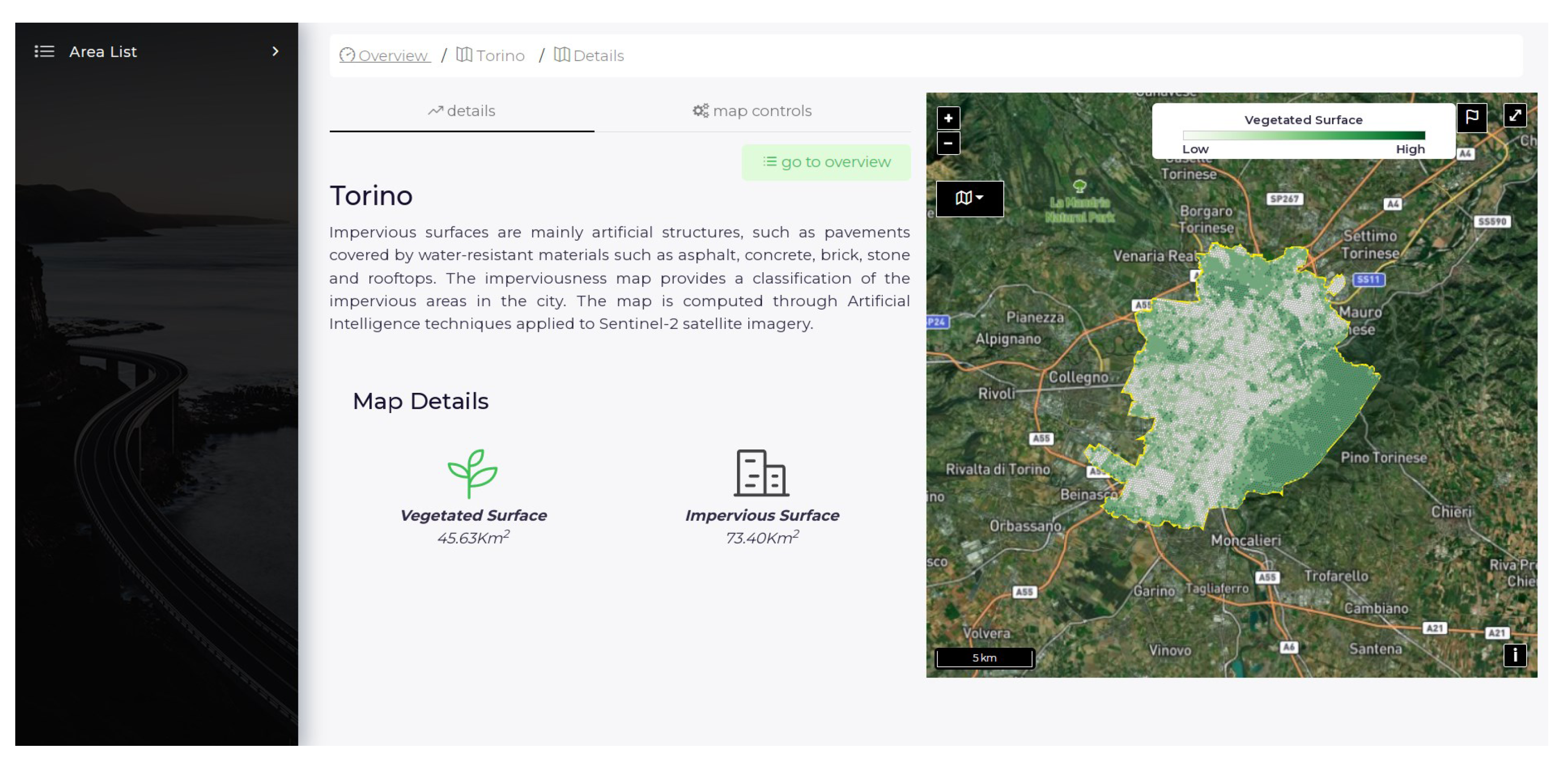
Additionally, as the work aims to realise a simple and effective tool, we integrated the proposed approach into a GIS web application. Figure 2 shows how requesting data for a specific area of interest can be simple, even for non-experts. In Figure 13, we share a web page we realised where the impervious data are presented to the end user using a map with a hexagonal grid. The grid was computed with a zonal statistics process applied to the imperviousness map computed through the proposed approach. The whiter areas represent the areas with the most impervious surfaces; vice versa, greener hexagons are the zones with the highest presence of trees, parks, and gardens. The image shows the map of impervious surfaces for the city of Turin in Italy. In particular, it shows how the areas with the highest content of impervious surfaces in the city centre can be easily identified, i.e., white hexagons.

In conclusion, the proposed approach shows how deep-learning, MLOPS and web-based application can effectively be used for a social-good application, such as imperviousness classification, in a simple and intuitive manner. The applicability of the proposed approach to different land-cover classification tasks will be tested to analyse the generalization capability of the approach across different applications. Finally, other experiments will be conducted, considering the time variable and extending the proposed dataset with new data sources, such as Sentinel-1 SAR satellite imagery.