Abstract
Determining the network size is a critical process in numerous areas (e.g., computer science, logistic, epidemiology, social networking services, mathematical modeling, demography, etc.). However, many modern real-world systems are so extensive that measuring their size poses a serious challenge. Therefore, the algorithms for determining/estimating this parameter in an effective manner have been gaining popularity over the past decades. In the paper, we analyze five frequently applied distributed consensus gossip-based algorithms for network size estimation in multi-agent systems (namely, the Randomized gossip algorithm, the Geographic gossip algorithm, the Broadcast gossip algorithm, the Push-Sum protocol, and the Push-Pull protocol). We examine the performance of the mentioned algorithms with bounded execution over random geometric graphs by applying two metrics: the number of sent messages required for consensus achievement and the estimation precision quantified as the median deviation from the real value of the network size. The experimental part consists of two scenarios—the consensus achievement is conditioned by either the values of the inner states or the network size estimates—and, in both scenarios, either the best-connected or the worst-connected agent is chosen as the leader. The goal of this paper is to identify whether all the examined algorithms are applicable to estimating the network size, which algorithm provides the best performance, how the leader selection can affect the performance of the algorithms, and how to most effectively configure the applied stopping criterion.
1. Introduction
1.1. Theoretical Background into Multi-Agent Systems
The term “multi-agent system” (MAS) is defined as a computer-based environment formed potentially by hundreds to thousands of interacting intelligent entities referred to as agents [1]. As the literature review shows [2,3,4], numerous experts from the computer science community provide various definitions of what the term “agent” means. In general, an agent of MAS is considered to be a part of a software/hardware computer-based system that exchanges messages with its peers as well as interacting with its surrounding environment [5,6]. Thus, the agents are able to learn novel actions and contexts, thereby being capable to make autonomous decisions [6]. One of the greatest advantages of the agents is their significant flexibility, making MASs applicable in many various fields such as diagnostics, civil engineering, power system restoration, market simulation, network control, etc. [3,6]. Besides, an agent of MAS is also characterized by other valuable features such as low cost, high efficiency, reliability, etc. and can take various forms—it is a software, hardware, pr hybrid (i.e., a combination of two previous) component [6] (see Figure 1 for a general structure of an agent forming MAS) [6].
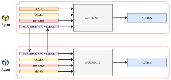
Figure 1.
General structure of agent forming multi-agent system.
Furthermore, as stated in [5], the agents of MASs can be characterized by four main features:
- □
- Autonomy is the ability to operate without any human interaction and to control its own actions/inner state.
- □
- Reactivity is the ability to react to a dynamic surrounding environment.
- □
- Social ability is the ability to communicate with other agents or human beings.
- □
- Pro-activeness is the ability to act as an initiative entity and not only to respond to an external stimulus.
All the mentioned benefits of the agents allow MASs to be applied to solving time-demanding and complex problems (often unsolvable by an individual agent) by splitting them into several simpler subtasks [6,7]. Thus, MAS can be understood as an interconnected computerized system of multi-functional entities interacting with each other in order to solve various complex problems in an effective manner. Therefore, MASs have been significantly gaining importance over the past decades [7].
1.2. Data Aggregation in Multi-Agent Systems
In our modern era, the amount of information is rapidly being increased in numerous industries whereby many modern systems benefit from the application of algorithms for data aggregation [8,9]. Data aggregation is a multidisciplinary research field addressing how to integrate data from independent multi-data sources into a more precise, consistent, and suitable form [10,11,12]. As stated in [9] and shown in Figure 2, there are many ways to classify the data aggregation methods.
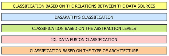
Figure 2.
Various classifications of data aggregation methods.
In this paper, we turn our attention to the classification based on the type of the system architecture. In this case, the data aggregation methods are divided into categories according to where (i.e., on which system component) data aggregation is executed. Namely, these four categories are defined by the authors of [9]:
- □
- Centralized architecture: Data aggregation is carried out by the fusion node, which collects the raw data from all the other agents in the system. Thus, all the agents measure the quantity of interest and are only required to deliver this information to the fusion node subsequently. Therefore, this approach is not too appropriate for real-world systems since it is characterized by a significant time delay, a massive transmitted information amount, high vulnerability to potential threats, etc.
- □
- Decentralized architecture: In this approach, there is no single point of data aggregation in contrast to the centralized architecture. In this case, each agent autonomously aggregates its local information with data obtained from its peers. Despite many advantages, decentralized architecture also has several shortcomings, e.g., communication costs, poor scalability, etc.
- □
- Distributed architecture: Each agent in a system independently processes its measurement; therefore, the object state is executed only according to the local information. This approach is characterized by a significant reduction of communication and communication cost, thereby gaining in popularity and finding a wide application in real-world systems over recent years [13,14,15,16].
- □
- Hierarchical architecture: This architecture (also referred to as hybrid architecture) is a combination of the decentralized and the distributed architecture, executing data aggregation at different levels at the hierarchy.
Even though the decentralized and the distributed architecture seem to be similar to one another, there are several differences between these two categories [9,17]. In this part, we turn the readers’ attention to the most significant contrasts. One of them is the fact that the measured data are pre-processed in the distributed architecture. Subsequently, a vector of features, which is then aggregated, is created as a result of this process. However, in the decentralized architecture, the data aggregation is completely executed at every agent in MAS whereby each agent can provide a globally aggregated output. Furthermore, in the decentralized architecture, information is commonly communicated, while, in the distributed one, the common notion of some states (position, identity, etc.) is shared. Besides, in decentralized architecture, it is an easy process to separate old information from the new one in contrast to the distributed one. On the other hand, the implementation of the decentralized architecture is generally considered to be more difficult. However, as shown in the literature [17,18], these two terms are often understood as synonyms and are therefore used as equivalents.
Note that one may find more general classifications according to the type of the system architecture [19]. As stated above, we focus our attention on distributed data aggregation mechanisms, a modern solution preferred in numerous modern applications (see Figure 3 for an example of the distributed architecture).
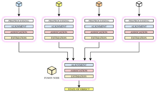
Figure 3.
Example of distributed architecture.
1.3. Consensus Theory
The problem of consensus achievement, an active research field with a long history in computer science, has been attracting great attention from both academia and industry over recent years [20]. In general, the term “consensus” means achieving an agreement upon a certain value determined by the inner states of all the agents in MAS [20,21]. In MASs, the term “consensus algorithm” (sometimes referred to as a consensus protocol) is understood as a set of rules specifying how the agents in MAS interact with their neighbors [20]. The goal of distributed consensus algorithms is to ensure agreement among a set of independent autonomous entities interconnected by potentially faulty networked systems [21]. Over the past decades, the consensus algorithms have found a wide range of applications in various fields such as wireless sensor networks, robotic systems, unmanned air vehicles, clustered satellites, etc. [19,21]. In this paper, we focus our attention on the distributed consensus algorithms, which are iterative schemes for determining/estimating various aggregate functions (e.g., the arithmetic mean, the sum, the graph order, the extreme, etc.).
The authors of [22] defined two categories of distributed consensus algorithms:
- □
- Deterministic algorithms include the Metropolis–Hastings algorithm, the Max-Degree weights algorithm, the Best Constant weights algorithm, the Convex Optimized weights algorithm, etc.
- □
- Gossip algorithms include the Push-Sum protocol, the Push-Pull protocol, the Randomized gossip algorithm, the Broadcast gossip algorithm, etc.
1.4. Our Contribution
In this paper, we analyze five frequently applied distributed consensus gossip algorithms with bounded execution for network size estimation. Namely, we choose these five algorithms for evaluation:
- □
- Randomized gossip algorithm (RG);
- □
- Geographic gossip algorithm (GG);
- □
- Broadcast gossip algorithm (BG);
- □
- Push-Sum protocol (PS); and
- □
- Push-Pull protocol (PP).
Our contribution is motivated by the lack of papers concerned with the applicability of these algorithms to network size estimation and their comparison. Our goal is to identify whether all the examined algorithms are applicable to estimating the network size, which algorithm is the best performing approach, how the leader selection can affect the performance of the algorithms, and how to most effectively configure the applied stopping criterion. In our analyses, the initial configuration of the applied stopping criterion is varied, either the best-connected or the worst-connected agent is the leader, and also the way to stop the algorithms differs. The algorithms are tested over 100 random geometric graphs (RGGs) each with a unique topology. The performance of the algorithms is quantified by applying two metrics, namely the number of sent messages required for consensus achievement and the estimation precision. Besides, the distribution of the number of sent messages is examined for each algorithm. Finally, we compare our conclusions made according to the presented experimental results with papers published by other authors and addressing the same algorithms.
1.5. Paper Organization
In Section 2, we provide papers published by other authors where the five examined algorithms are compared and analyzed. In Section 3, we present the used model of MAS. In Section 4, the analyzed algorithms are introduced. In Section 5, we present the applied research methodology and the metrics used to evaluate the performance of the analyzed algorithms. In Section 6, we present the results from the numerical experiments and compare our conclusion with related papers. Section 7 briefly summarizes the outputs of our research.
2. Related Work
In this section, we deal with papers concerned with distributed consensus gossip-based algorithms published by other authors. We focus our attention on papers (or their parts) where the algorithms that we analyze in this paper are compared.
The authors of [23] compared BG and RG using the simulator Castalia and by applying several metrics, namely the communication overhead, the latency, the energy consumption, the normalized absolute error, and the standard deviation. In addition, three different sets of the initial states are assumed in the presented research. They identified that BG in general achieves a greater performance than RG. BG achieves low performance only in terms of the normalized absolute error. As in the previously discussed manuscript, BG and RG are also compared in [24], however, under quantized communication in this case. In this paper, it is identified that BG outperforms RG in terms of the time required to achieve the quantized consensus over various network types, namely random geographical spatial networks with the same connectivity radius, small-world networks, and scale-free networks. The authors of [25] also focused their attention on a comparison of BG with RG and identified that BG outperforms RG in both the convergence time and the number of radio transmissions regardless of the network size. In [26], the authors examined and compared three gossip algorithms (BG, RG, and GG) by applying several metrics. They identified that BG outperforms the two other examined algorithms in terms of the per-node variance. It is furthermore concluded in the paper that GG performs better in terms of the mentioned metric than RG in large-scale networks. However, in smaller networks, RG achieves better performance than GG. In the paper, an analysis of the algorithms in terms of the per-node mean square error is also provided. In this case, an interesting phenomenon is identified by the authors: the error of BG does not drop below a specific threshold in contrast to the two other algorithms, the precision of which is increased with no bound as the number of radio transmissions increases. For fewer radio transmissions, BG outperforms the two other algorithms, but, for higher values, it is the worst-performing algorithm among the analyzed ones—in this case, RG achieves the lowest per-node mean square error. The same conclusion regarding the per-node variance as in the previous paper was also reported by Spano [27]. Wang [28] compared RG and GG in terms of the error in estimation. They identified that GG outperforms RG regardless of the network size except for the scenarios where low energy is spent. Moreover, it is identified in the paper that the more energy is spent, the higher precision of the estimation is achieved. In [29], RG and GG are compared in terms of the relative error under various initial inner states over RGGs and grid graphs. In RGGs, GG outperforms RG in all the realized scenarios except for low values of the number of transmissions. In grid topologies, GG is better for each value of the number of the transmission.
In this paragraph, we turn our attention to papers dealing with PS and PP. In [30], the authors compared the mentioned algorithms in terms of the convergence rate expressed as the root mean square error as a function of rounds under asynchronous and potentially faulty environments. They identified that PS is slightly outperformed by PP for a lower number of rounds. However, when the round number is equal to approximately 60, PS achieves higher performance than PP. In [31], very similar research to the one from [30] is carried out. In [31], PS outperforms PP also for lower values of iterations. Spano [32] compared PP and PS by applying the mean percentage error and the variance. It can be observed in the paper that PP outperforms PS for a lower number of rounds, but PS performs better for a greater number of rounds. The variance is greater in the case of PS. The authors of [33] identified that PS outperforms PP in terms of the mean least absolute percent error. Moreover, they showed that PS achieves worse performance only in large-scale networks with a low mean degree. PS is better than PP also in terms of the mean number of rounds except for large-scale networks with a high mean degree. It is furthermore shown in the paper that PS outperforms PP in terms of the mean number of wasted rounds in each analyzed scenario. In terms of the number of sent messages, PS achieves a greater performance than PP in all the executed scenarios.
In [34], the authors introduced a distributed algorithm based on Extrema Propagation, which is general considered to be a fast and fault-tolerant approach for estimating the network size. In the presented algorithm, each agent generates a vector containing random numbers (generated data have a known probability distribution). Then, the data are aggregated (an obtained value has a distribution dependent on the network size) over the whole network by applying a pointwise minimum, an idempotent operation. Afterward, the resulting vector as a sample is used to infer the number of the nodes. In contrast to this approach, PP is used to estimate the arithmetic mean, from which the network size is then estimated (it is equal to the inverse value of the arithmetic mean estimate). In this algorithm, the initial inner states are equal to either “1” or “0”, and one of the agents has to be selected as the leader. Thus, in [34], it is shown that there are also other ways to estimate the network size.
As shown in [35,36], network size estimation is an important process in many areas such as charging electric vehicles, social Internet of vehicles, etc.
Thus, as seen in the provided literature review, the papers addressing distributed consensus gossip algorithms are primarily focused on the problem of distributed averaging. Thus, there is a lack of papers concerned with an analysis of RG, GG, and BG for network size estimation. The two other chosen algorithms (i.e., PS and PP) for this purpose are briefly discussed in [30,34,37,38,39,40,41,42]. However, in none of these papers, a comprehensive analysis of these algorithms applied to estimating the network size is provided. Besides, a deep comparison of all the five algorithms is not found in the literature.
3. Mathematical Model of Multi-Agent Systems
In this paper, MASs are modeled as simple finite undirected unweighted graphs labeled as G and determined by two time-invariant sets, namely the vertex set V and the edge set E (G = (V, E)) [43,44]. The vertex set V consists of all the graph vertices representing the agents in MAS. The cardinality of this set determines the graph order (labeled as n), i.e., the number of agents in MAS. Each vertex from V is allocated a unique index, a positive integer value from the range [1, n], i.e., V = {v, v, … , v}. The other set, the edge set E⊂V×V, is formed by all the graph edges, which represent a direct link between two vertices. The cardinality of the edge set E determines the size of the corresponding graph G, i.e., the overall number of direct connections in MAS. The direct link between two agents v and v (i.e., their distance is one hop) is indicated by the existence of an edge in G labeled as e. Every two vertices directly linked to one another are said to be neighbors. Subsequently, the set containing all the neighbors of an agent v can be defined as:
In this paper, we examine the chosen algorithms over RGGs, graphs that represent spatial MASs with n randomly deployed agents [43,44] (see Figure 4 for an example of RGGs (one of 100 RGGs applied in our research is shown in this figure to illustrate what the network topology of the used graphs looks like) and Table 1 containing the graph parameters (the average value of each parameter of 100 applied graphs is shown)). In these graphs, the agents are placed uniformly at random over a square area of finite size. Subsequently, two agents are directly linked to one another, provided their distance is not greater than the transmission radius (each agent has the same transmission radius). In the case that there is a path between each pair of two vertices, we say that this graph is connected. If not, the graph is disconnected, thereby being composed of two or more components. Different connectivity in a graph can be ensured by modifying the value of the transmission radius. As shown in the literature [22,34,45,46], this graph type is often applied to modeling real-world systems such as wireless sensor networks, ad-hoc IoT networks, social networks, etc. The algorithm used to generate RGGs applied in our research can be described as follows: in the beginning, we have a blank working area formed by 150 points on both the x- and the y-axis. Thus, there are 150 coordinates (x,y) in the working area. Then, the first vertex is placed uniformly at random on one of these coordinates (i.e., it can be placed on each coordinate with the same probability equal to 1/150). Afterward, the other vertices (one by one) are placed on free coordinates—one coordinate can be allocated to only one vertex. Once all the vertices are distributed over the working area (200 vertices in overall in our case), edges linking all the adjacent vertices are added to the graph. As mentioned earlier, two vertices are linked to one another, provided that their distance is not greater than their transmission radius.
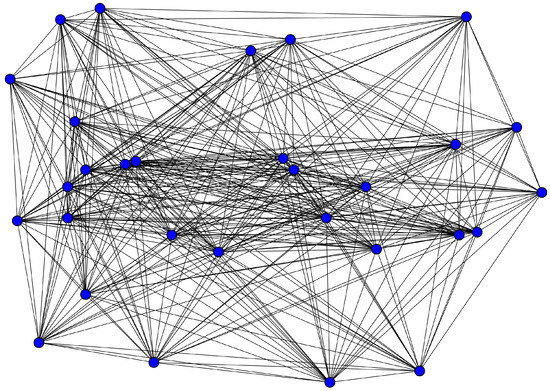
Figure 4.
Example of random geometric graphs used in our experiments.

Table 1.
Graph parameters of 100 RGGs used in our experiments.
4. Examined Distributed Consensus Gossip-Based Algorithms
In this section, we introduce all the distributed consensus gossip-based algorithms chosen for evaluation in our research presented in this paper. We analyze five frequently cited approaches primarily proposed for estimating arithmetic mean, namely we examine these algorithms:
- □
- Randomized gossip algorithm (RG): see Section 4.1.
- □
- Geographic gossip algorithm (GG): see Section 4.2.
- □
- Broadcast gossip algorithm (BG): see Section 4.3.
- □
- Push-Sum protocol (PS): see Section 4.4.
- □
- Push-Pull protocol (PP): see Section 4.5.
Furthermore, as stated above, we compare these five algorithms for not very frequently applied functionality—distributed network size estimation. In each algorithm, the agents of MAS initiate their inner state (or the variable sum in the case of PS) with, e.g., locally measured information in the case of distributed averaging or distributed summing. The vector gathering the inner states (representing arithmetic mean estimates) of all the agents at a time instance k is labeled as x(k), the inner state of v at a time instance k is labeled as x(k), and x(0) is a label of the initial inner state of v. However, in the case of distributed network size estimation, exactly one of the agents has to be selected as the leader—for example, the agent at which the query is inserted [47]. The initial inner state of the leader is equal to “1”, while all other agents set their initial inner state to “0”. In our experiments, either the best-connected or the worst-connected agent is chosen as the leader in order to identify the impact of the leader selection on the performance of the algorithms. Thus, the inner states of all the agents approach (n is equaled to 200 in our experiments) as the number of time instances is increased. Thus, the agent can easily estimate the network size at each time instance as follows:
Thus, in our experiments, NSE approaches 200 and x(k) 1/200. The vector gathering all the estimates at a kth time instance is labeled as NSE(k). We refer to the states/the estimates after the consensus among all the agents in MAS is achieved as the final inner states/the final estimates. Figure 5 shows an example of how the inner states/the network size estimates differ before and after any examined algorithm for network size estimation is executed.
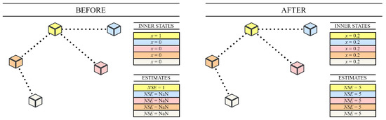
Figure 5.
Comparison of inner states/arithmetic mean estimates before and after consensus is achieved in multi-agent system.
4.1. Randomized Gossip Algorithm
The first analyzed algorithm is RG, where one of the agents is woken up (this agent is selected from all the agents in MAS uniformly at random—let us label it as v) at each time instance k and chooses one of its adjacent neighbors (i.e., one of the agents from —let it be labeled as v) [22,26,48]. Subsequently, these two agents exchange their current inner and execute the pairwise averaging operation [22]:
The inner states of the agents that do not send/receive any message at a time instance are not updated at this time instance. Thus, all other agents except for those that perform the pairwise averaging operation (3) use their current inner state also for the next time instance. In [48], it is identified that the consensus is achieved, provided that the graph is strongly connected on average. As stated in [26], this algorithm poses a vulnerable and communication-demanding approach.
4.2. Geographic Gossip Algorithm
Another analyzed approach is GG, the principle of which lies in the combination of gossiping with geographic routing mechanisms [28]. As in the case of the previous algorithm, at each time instance k, one of the agents is woken up and selects one of the agents from the whole network (except for itself) uniformly at random [26,28]. Subsequently, these two agents perform the pairwise averaging operation (3). Thus, the main idea of this approach is that an agent can perform the pairwise averaging operation with agents further than one hop [28]. Thus, one of the most serious drawbacks of this approach is the necessity to know the geographical information about the agents [26,28]. However, the diversity of pairwise exchanges is significantly increased compared to the previous algorithm whereby data aggregation is assumed to be optimized [26]. In our experiments, we assume the optimal routing, i.e., the messages are always transported to the addressee by the shortest path.
4.3. Broadcast Gossip Algorithm
The next examined algorithm is BG, whose principle can be described as follows: at each time instance k, one of the agents (let us refer to it as v) is selected uniformly at random [22,26]. Subsequently, this agent broadcasts its current inner states to all its neighbors, which updates their inner states as follows [26]:
Here, is the mixing parameter taking a value from the following interval [26]:
In our analyses, its value is set to 0.9. The inner state of all the other agents (including the broadcasting one) for the next time instance is determined as follows [26]:
Thus, this algorithm does not require a pairwise communication whereby it is significantly simplified in contrast to the two previous approaches. However, as shown in [26], the precision of BG can be much lower than the precision of concurrent approaches as the inner states may not approach the value of the estimated aggregate function.
4.4. Push-Sum Protocol
In this paper, PS is also chosen for evaluation. In this algorithm, every agent has to store and update two variables [47]:
- □
- sum s (initiated with either “1” (leader) or “0” (other agents) when the network size is estimated); and
- □
- weight w (each agent sets its value to “1”).
The principle of this algorithm can be described as follows [47]: at each time instance k, each agent in a system selects one of its neighbors uniformly at random and sends it half of its sum and half of its weight, both for the current time instance (we assume that the agents are synchronized; therefore, no collisions may occur while the messages are sent). In addition, the same values are stored in its memory. Each agent v can estimate the arithmetic mean (labeled as x(k)—this parameter is equivalent to the inner states in the other algorithms) at each time instance k as follows:
The sum s for the next time instance (i.e., s(k + 1)) is determined by the sum of all the received sums from other agents at a time instance k with half of its own sum at a time instance k. Analogically, the weight for the next time instance (i.e., w(k + 1)) is equal to the sum of all the received weights from other agents at a time instance k with half of its own weight at a time instance k. As stated in [47], the proper operation of PS is ensured, provided that the total system mass is preserved constant. Thus, losing messages causes that algorithm to not operate correctly [34].
4.5. Push-Pull Protocol
The last analyzed algorithm is PP, where each agent periodically (i.e., at each time instance k) sends a message containing its current inner state (referred to as a Push message) to one of its neighbors chosen uniformly at random [3,34]. The message receiver answers with its current inner state (a so-called Pull message) so that these two agents can perform the pairwise averaging operation [3,34]. Similar to the previous approach, PP is very sensitive to losing messages [34]. Again, the agents are assumed to be synchronized, so no collisions may occur while the messages are sent.
4.6. Comparison of Distributed Gossip Consensus Algorithms with Deterministic Ones
As mentioned above, we focus our attention on the gossip algorithms, where the message receivers are chosen randomly in contrast to the deterministic algorithms. Thus, many parameters of the gossip algorithms vary over the runs—in Figure 6, we provide the evolution of arithmetic mean estimates of the Push-Sum protocol (gossip algorithm) and the Max-Degree weights algorithm (deterministic algorithm) for three independents runs of the algorithms in order to demonstrate differences between these two categories.
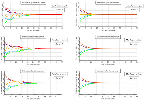
Figure 6.
Comparison of gossip Push-Sum protocol with deterministic Max-Degree weights algorithm over three runs—evolution of arithmetic mean estimates.
The Max-Degree weights algorithm is s a deterministic distributed consensus algorithm operating in synchronous mode [49]. It requires the exact value of the maximum degree of a graph (i.e., the degree of the best-connected agent in MAS) for the proper operation. In this algorithm, this parameter determines the value of the mixing parameter , i.e., all the graph edges are set to the value of this parameter. The update rule of this algorithm is defined as follows [49]:
Here, W is the weight matrix of this algorithm, a doubly-stochastic matrix defined as follows [49]:
Here, d is the degree of v. The principle of this algorithm can be described as follows: at each time instance, each agent broadcasts its current inner states to all its neighbors as well as receiving the inner states from them. Subsequently, it multiplies all received data and its current inner state with the allocated weights (as shown in (9)). The sum of all these values represents its inner state for the next time instance.
Figure 6 shows that the evolution of the estimates is the same for each run in the case of the deterministic Max-Degree weights algorithm, while the estimates may differ in the case of the Push-Sum protocol. In both cases, the estimates, however, approach the value of the arithmetic mean (=3 in this case), which is the most important fact.
In Figure 7, we show the distribution of the convergence rates (a stopping criterion is applied) for 100,000 runs for both algorithms. As seen, the convergence rates are the same for each run in the case of the Max-Degree weights algorithm. However, when the Push-Sum Protocol is applied, the convergence rates may differ from each other for various runs, and the distribution evokes a Gaussian distribution.
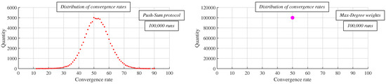
Figure 7.
Comparison of gossip Push-Sum protocol with deterministic Max-Degree weights algorithm—distribution of convergence rate over 100,000 runs.
5. Applied Research Methodology
In this section, we draw our attention to the methodology applied in our research and the metrics used to evaluate the performance of the algorithms chosen for an examination.
As mentioned above we carry out two extensive experiments differing from each other in the way to bound the algorithms:
- □
- Scenario 1: In this scenario, the value of the current inner states is relevant in the decision about whether or not to stop an algorithm at the current time instance. This stopping criterion is defined in (10), meaning that an algorithm is stopped at the time instance when (10) is met for the first time.
- □
- Scenario 2: In the case of applying the other applied stopping criterion, the values of the current network size estimates are checked instead of the inner states. In this scenario, the consensus is considered to be achieved when (11) is met.
The time instance when (10) or (11) is met for the first time is labeled as k. Once the conditions (10) and (11) are met, the agents forming MAS are said to have achieved consensus. Thus, the algorithms are completed.
Here, P is the parameter determining when to stop an algorithm. Its higher values mean that the difference between the inner states/the network size estimates is greater after the consensus is achieved. In our experiments, it takes the following values: {0.1, 0.01, 0.001, 0.0001}.
In this paragraph, we justify why we choose these two scenarios for evaluation. In Scenario 1, the arithmetic mean is estimated, and then network size estimates are determined by applying (2). Thus, the consensus achievement among the agents is conditioned by the arithmetic mean estimates. In this scenario, the consensus among the agents is achieved, provided that the difference in the absolute value between the maximum and the minimum from all the current arithmetic mean estimates is smaller than the parameter P. Unlike this scenario, consensus achievement is conditioned by the current network size estimates in Scenario 2. Therefore, in this case, consensus among the agents is achieved if the difference in the absolute value between the maximum and the minimum from all the current network size estimates is smaller than the parameter P.
In Figure 8 and Figure 9, we compare RG in both scenarios. The figures show that the algorithm is faster in Scenario 1, but the precision of the final estimates of the network size (the network size is 5 in this case) is lower than in Scenario 2.
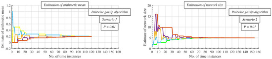
Figure 8.
Comparison of evolution of arithmetic mean estimates with evolution of network size estimates—pairwise gossip algorithm is applied.
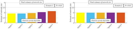
Figure 9.
Comparison of final network size estimates in both examined scenarios—pairwise gossip algorithm is applied.
As shown in [50], where distributed deterministic consensus algorithms are analyzed, the selection of the leader can affect the performance of algorithms for the network size estimation. Thus, we carry out two analyses in order to examine the impact of the leader selection on the performance of the examined algorithms:
- □
- The best-connected agent is the leader.
- □
- The worst-connected agent is the leader.
To evaluate the performance of the chosen algorithms, we apply two metrics, namely the number of sent messages required for consensus achievement and the median deviation of the final estimates from the real value of the network size. We do not apply the frequently applied metric—the number of time instances for consensus—as the number of sent messages per time instance differs for various algorithms. In the case of RG, two messages are sent at each time instance. When GG is used, the number of sent messages per time instance is equal to twice the distance between the two agents performing the pairwise averaging operation. If BG is applied, the number of sent messages per time instance equals one. In the case of PS, n messages are sent per time instance, and twice n messages are transmitted when PP is used. The precision of estimation is determined as the median deviation of the final estimates of all the agents from the real network size (the median is chosen instead of the average since the final inner state of some agents can be equal to zero whereby their final estimate is NaN). Its formula (for each algorithm same) is defined as follows:
As the algorithms are gossip, both metrics vary over runs; therefore, each algorithm is repeated 100 times in each graph. Subsequently, the median of these values is chosen as a representative of a corresponding metric in a graph.
In addition, as mentioned above, we analyze the algorithms over RGGs—to ensure high credibility of our research, we generate 100 graphs of unique topology each and with the graph order n = 30. All generated graphs are connected because the algorithms can be applied to estimating the network size only under this circumstance (in the disconnected graphs, the size of the components is estimated instead of the network size). In Figure 10, Figure 11, Figure 12 and Figure 13, we show the median of representatives of both metrics over 100 graphs.

Figure 10.
Comparison of the number of sent messages required for consensus achievement of all algorithms in both scenarios for various configurations of implemented stopping criterion—best-connected agent is leader.

Figure 11.
Comparison of the estimation precision of all algorithms in both scenarios for various configurations of implemented stopping criterion—best-connected agent is leader.
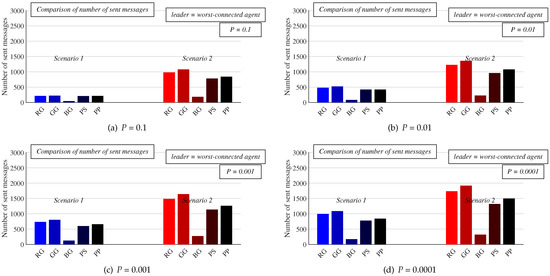
Figure 12.
Comparison of the number of sent messages required for consensus achievement of all algorithms in both scenarios for various configurations of implemented stopping criterion—worst-connected agent is leader.
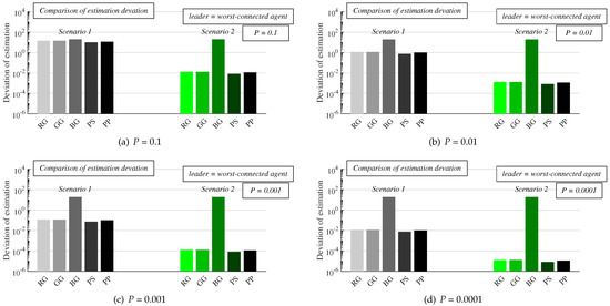
Figure 13.
Comparison of the estimation precision of all algorithms in both scenarios for various configurations of implemented stopping criterion—worst-connected agent is leader.
In the last experiment, the results of which are shown in Figure 14, each algorithm is repeated 10,000 times in one of the graphs (each algorithm in the same graph) in order to examine the distribution of the number of sent messages required for consensus achievement.
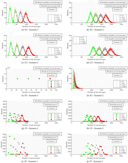
Figure 14.
Distribution of number of sent messages in both scenarios for various configurations of implemented stopping criterion and with the best-connected agent as leader.
Regarding the value of the mixing parameter of BG, we set this value to 0.9 as this configuration ensures the highest estimation precision compared to the other mixing parameters to the nearest tenth.
As shown in [51], the algorithms can also be analyzed by applying the topological distance. This kind of analysis is involved in our future plans.
6. Experiments and Discussion
In this section, we present and discuss the results of numerical experiments executed in Matlab 2018a. We use either software proposed by the authors of this paper or Matlab built-in functions. This section is partitioned into two subsections:
- □
- Experiments: In this subsection, we present the results from numeral experiments for each examined algorithm. In Figure 10 and Figure 11, we provide the number of sent messages for consensus and the estimation precision, respectively, in both scenarios, for four values of the parameter P, and with the best-connected agent selected as the leader. In Figure 12 and Figure 13, the results obtained in experiments with the worst-connected agent as the leader are provided. In Figure 14, the distribution of the sent messages over 10,000 runs for each algorithm, in both scenarios, for each value of P, and with the best-connected agent selected as the leader is provided.
- □
- Discussion: In this subsection, we compare the results presented in Section 6.1 with conclusions presented in the papers from Section 2.
6.1. Experiments
In our experiments, we assume that there are no potential failures negatively affecting the execution of the algorithms (e.g., communication breakdowns, deaths of agents, misbehavior of agents, etc.), and the communication is not affected by any noise worsening the quality of the transmitted messages. In addition, all the agents are assumed to be homogenous in the transmission range, communication, computation capabilities, and other aspects affecting the execution of the algorithms.
At first, we focus our attention on an analysis of the number of sent messages in Scenario 1 with the best-connected agent selected as the leader. From the results depicted in Figure 10 (blue bars), it can be seen that a decrease in P results in an increase in the number of sent messages for each analyzed algorithm. Thus, the best performance of all examined algorithms in terms of the number of sent messages is achieved when the value of P is equal to 0.1. In addition, the highest performance is achieved by BG, which significantly outperforms all the other algorithms for each value of P. Besides, a decrease in P has only a marginal impact on the performance of BG in contrast to the other algorithms—the sent messages take the values from this interval [22, 88]. In addition, a decrease in P ensures that the difference in the performance between BG and the other algorithms is increased. The second-best performing algorithm is PS followed by PP, the third-best performing algorithm. However, the difference between these two algorithms in the number of sent messages required for consensus is almost negligible except for lower values of P. The sent messages are from the interval [180, 780] in the case of PS and from [180, 840] in the case of PP. Thus, these algorithms require much more messages for consensus than previously discussed BG. The fourth best-performing is RG, the sent messages of which are from the following interval [193.5, 968]. The worst performance is achieved by GG, whose sent messages take the following values [225, 1085]. Moreover, it is seen that a decrease in P causes that the difference in the performance between these algorithms and the difference between these two algorithms and the others to increase.
As mentioned above, we compare two scenarios determining the way to bound the algorithms in order to identify whether it is better to stop the algorithms according to the current arithmetic mean estimates or the current network size estimates. The results presented in this paragraph and their comparison with those from the previous one help identify the optimal way to bound the algorithms. In the following, we turn our attention to Scenario 2, and the sent messages required for consensus achievement with the best-connected agent selected as the leader are analyzed again. Thus, in this paragraph, we present the results of the same experiments as in the previous one with the difference that the stopping criterion (11) is applied instead of (10). The purpose of this analysis is to identify the optimal way to bound the algorithms. The results for Scenario 2 are shown in Figure 10 (red bars). Again, it is seen that a decrease in P results in an increase in the number of sent messages regardless of the applied algorithm. As in Scenario 1, the best performance is achieved by BG (the number of sent messages is from the interval [100.5, 167.5], and the value of P has only a marginal impact on the performance of BG), the second-best by PS ([780, 1320]), the third-best by PP ([840, 1440]), the fourth-best by RG ([955, 1717]), and the worst performance is achieved by GG ([1078, 1923]). Again, a decrease in P causes that the difference in the performance between the algorithms to increase. Compared to Scenario 1, the algorithms require many more sent messages for consensus—in the case of RG, the difference between Scenario 1 and Scenario 2 in the number of sent messages is around 750 messages, around 840 in the case of GG, around 80 when BC is applied, around 540 if PS is used, and around 630 in the case of PP. Moreover, it is observed that the value of P has only a marginal impact on the value of this difference.
We next turn the readers’ attention to the precision of the network size estimation (see Figure 11). As mentioned above, we quantify this parameter by applying the median deviation defined in (12). At first, we focus on Scenario 1 with the best-connected agent as the leader (grey bars)—from the results, we can see that a decrease in P ensures a lower deviation of each analyzed algorithm whereby a higher precision of the final estimates is achieved. In contrast to the previous analyses, the algorithm requiring the lowest number of sent messages for consensus achievement, BG, is significantly outperformed by all the four other algorithms. Its deviation is from the range [32.95, 52.25] agents; therefore, its precision is so low that this algorithm is not applicable to estimating the network size for any P in Scenario 1. The four other algorithms do not significantly differ from each other in the estimation precision, but their precision is also very low (the median deviation is around 12 agents) for P = 0.1. In the case of P = 0.01, the median deviation is around one agent, which is a significantly more precise estimation compared to the previous case. Nevertheless, even this configuration is not appropriate for real-world applications requiring the exact value of the network size. Very high precision of the final estimates is achieved in the case of P = 0.001 (the median deviation is equal to around 0.1 agents) and P = 0.0001 (the median deviation is approximately 0.01 agents). Thus, only these two configurations of the stopping criterion can ensure estimation of the network size with high precision in Scenario 1.
We next focus on the precision of the final estimates in Scenario 2 with the best-connected agent as the leader (see green bars in Figure 11). As seen from the results, a decrease in P ensures a higher precision of the final estimates as in Scenario 1. In this scenario, the precision of BG is higher (the deviation is from the interval [32.52, 37.66] agents) compared to Scenario 1, but it is still very low. Thus, BG is useless in both scenarios and is, therefore, not applicable to estimating the network size at all. Conversely, the precision of the four other algorithms is very high for each P in this scenario, and, again, there is no significant difference between these algorithms in terms of the estimation precision. Even for P = 0.1, the deviation is low—the median deviation is approximately 0.01 agents. The lowest deviation is achieved for P = 0.0001, taking the value around 10 agent. Thus, the estimation precision is much greater in Scenario 2 than in Scenario 1—except for BG, the deviation is about three orders of magnitude lower, and P has only a marginal impact on this difference.
In Figure 12 and Figure 13, the same experiments are repeated, but the worst-connected agent is selected as the leader instead of the best-connected one. As seen, the number of sent messages is slightly increased compared to scenarios with the best-connected agent chosen as the leader, while the deviation of the final estimates from the real network size is slightly decreased. However, there is no significant difference in the values of both applied metrics when the worst-connected agent is selected as the leader instead of the best-connected one. As further observed from the results, the most affected algorithms are RG and BG. Thus, the selection of the leader has only a marginal impact on the performance of distributed consensus gossip algorithms in contrast to deterministic ones, the performance of which is intensively affected by the leader selection, as identified in [50].
In the last part, we analyze the distribution of the number of sent messages—the algorithms are carried out in one of the graphs 10,000 times in both scenarios and for each value of P as mentioned above. Since the number of sent messages is only marginally affected by the leader selection, we carry out only Scenario 1 (i.e., with the best-connected agent selected as the leader). The goal of this experiment is to identify how the number of sent messages differs over various runs of the algorithms. From the results shown in Figure 14, we can see that the number of sent messages in the cases of RG (Figure 14a,b) and GG (Figure 14c,d) has a Gaussian distribution in both scenarios and for each P. In addition, this distribution is slightly skewed to the right in all four figures. In addition, the data in each figure are more spread as the value of P is decreased. The next analyzed algorithm is BG (Figure 14e,f), in which case we can see an interesting phenomenon—the number of sent messages does no differ over various runs in Scenario 1. Such behavior is usually observed when a distributed deterministic consensus algorithm is analyzed (Figure 7). However, in Scenario 2, the data differ for various runs as in the case of the two previous algorithms and has a significantly right-skewed Gaussian distribution. As in the cases of the two previously analyzed algorithms, a decrease in P causes that data are more spread, but not as significantly as in the cases of RG and GG. Finally, the two remaining algorithms, PS and PP (see Figure 14g–j), are analyzed. It can be seen in the figures that the data of both algorithms have a Gaussian distribution, again with right skewness. Compared to RG and GG, the data do not vary for various runs as significantly as in the case of the first two analyzed algorithms. Again, as in the case of the three previous algorithms, lower values of P result in greater data dispersion.
6.2. Discussion
In this section, we discuss the results presented in Section 6.1 and compare them with those from Section 2 in order to compare the examined algorithms for distributed averaging with their application to distributed network size estimation.
As shown in [23,24,25,26,27,28,29], BG outperforms RG and GG in terms of numerous various metrics. However, in [26], it is identified that the error of BG cannot drop below a threshold value whereby BG is outperformed by RG and GG for a higher number of time instances. This fact causes that BG requires the lowest number of sent messages for consensus achievement (significantly lower than the other algorithms), but its estimation precision is so low that this algorithm cannot be applied to estimating the network size—very low precision is achieved in all our experiments. Thus, a high convergence rate of BG at the cost of lower estimation precision can be beneficial if the arithmetic mean is estimated. However, in the case of network size estimation, its low precision makes this algorithm inapplicable to estimating the network size. Furthermore, it is shown in many papers that GG performs better than RG in numerous scenarios. However, in our analyses, GG requires the most sent messages for consensus achievement and thus is worse for network size estimation than RG. In GG, many redundant messages are often transmitted as two agents many hops away from one another with zero inner states perform the pairwise averaging operation (3). In our experiments, it is identified that these two algorithms achieve high precision in general and therefore can be used to estimate the network size in real-world systems.
As shown above, a comparison of PS and PP both for distributed averaging is provided in [30,31,32,33]. Generally, it is identified that PS outperforms PP except for several scenarios. In addition, the application of these algorithms to estimating network size is discussed in [30,34,37,38,39,40,41,42], but a comprehensive analysis is provided in none of them. In our research, it is identified that there is no significant difference between these two algorithms (PS performs a bit better), their precision is high in general, and they require fewer messages for consensus than RG and GG.
In addition, our research identifies that the selection of the leader has only a marginal impact on the performance of all the five algorithms. According to the presented results, we can conclude that the best-performing algorithm for network size estimation is PS, which requires the second-lowest number of sent messages for consensus, and its estimation precision is very high (except for cases when P takes high values in Scenario 1). The best performance of all the four applicable algorithms is achieved for P = 0.001 in Scenario 1, where the estimation precision is high, and the number of sent messages is lower than in Scenario 2 or in Scenario 1 with P = 0.0001. It is further identified that the precision in Scenario 2 is much higher than in Scenario 1 but at the cost of a significant increase in the number of sent messages.
7. Conclusions
In this paper, we analyze five frequently cited distributed consensus gossip algorithms (RG, GG, BG with = 0.9, PS, and PP), which are bounded by a stopping criterion determined by the parameter P, for minor application—distributed network size estimation. We analyze their performance over RGGs in two scenarios—the consensus achievement is conditioned by either the inner states (Scenario 1) or the network size estimates (Scenario 2). Besides, in both scenarios, either the best-connected or the worst-connected agent is selected as the leader. From the results presented in Section 6.1, it can be seen that a decrease in P ensures higher estimation precision of every analyzed algorithm, however, at the cost of an increase in the number of sent messages for consensus in both scenarios. The lowest number of sent messages for consensus is required by BG, but the precision of this algorithm is very low. Thus, this algorithm is not applicable to estimating the network size in any of the analyzed scenarios. All four other algorithms achieve high precision except for two configurations of the applied stopping criterion: P = 0.1 in Scenario 1 and P = 0.01 in Scenario 1. Overall, the best performance is achieved by PS, whose precision is the highest (a bit greater than the precision of RG, GG, and PP), and the number of sent messages is the second-lowest among the examined algorithms. In addition, we identify that the algorithms are more precise in Scenario 2 but require many more sent messages for consensus than in Scenario 1. Besides, it is shown that the selection of the leader has only a marginal impact on all the analyzed algorithms. Regarding the distribution of the sent messages, all the examined algorithms have a Gaussian distribution skewed to the right except for BG in Scenario 1, where the number of sent messages does not differ over runs. Moreover, it is identified that lower values of P cause a greater dispersion. According to the presented results and their analysis, we conclude that the best performance for all the four applicable algorithms is achieved for P = 0.001 in Scenario 1. Thus, this configuration is recommended by us for real-world systems.
Author Contributions
Conceptualization, M.K. and J.K.; methodology, M.K.; software, M.K.; validation, M.K., and J.K.; formal analysis, M.K. and J.K.; investigation, M.K.; resources, M.K.; data curation, M.K. and J.K.; writing—original draft preparation, M.K.; writing—review and editing, M.K. and J.K.; visualization, M.K.; supervision, J.K.; project administration, M.K.; and funding acquisition, M.K. All authors have read and agreed to the published version of the manuscript.
Funding
This work was supported by the VEGA agency under the contract No. 2/0155/19 and by the project CHIST ERA III (SOON) “Social Network of Machines”. Since 2019, Martin Kenyeres has been a holder of the Stefan Schwarz Supporting Fund.
Data Availability Statement
The data presented in this study are available on request from the corresponding author.
Acknowledgments
We would like to thank the anonymous reviewers of this paper for their supportive and insightful comments.
Conflicts of Interest
The authors declare no conflict of interest.
Abbreviations
The following abbreviations are used in this manuscript:
| BG | Broadcast gossip algorithm |
| GG | Geographic gossip algorithm |
| MAS | Multi-agent system |
| NaN | Not a Number |
| PP | Push-Pull protocol |
| PS | Push-Sum protocol |
| RG | Randomized gossip algorithm |
| RGG | Random geometric graph |
References
- Zheng, Y.; Zhao, Q.; Ma, J.; Wang, L. Second-order consensus of hybrid multi-agent systems. Syst. Control Lett. 2019, 125, 51–58. [Google Scholar] [CrossRef]
- McArthur, S.; Davidson, E.M.; Catterson, V.M.; Dimeas, A.L.; Hatziargyriou, N.D.; Ponci, F.; Funabashi, T. Multi-agent systems for power engineering applications—Part I: Concepts, approaches, and technical challenges. IEEE Trans. Power Syst. 2007, 22, 1743–1752. [Google Scholar] [CrossRef]
- Shames, I.; Charalambous, T.; Hadjicostis, C.N.; Johansson, M. Distributed Network Size Estimation and Average Degree Estimation and Control in Networks Isomorphic to Directed Graphs. In Proceedings of the 50th Annual Allerton Conference on Communication, Control, and Computing, Allerton, Monticello, IL, USA, 1–5 October 2012; pp. 1885–1892. [Google Scholar]
- Seda, P.; Seda, M.; Hosek, J. On Mathematical Modelling of Automated Coverage Optimization in Wireless 5G and beyond Deployments. Appl. Sci. 2020, 10, 8853. [Google Scholar] [CrossRef]
- Wooldridge, M.; Jennings, N.R. Intelligent agents: Theory and practice. Knowl. Eng. Rev. 1995, 10, 115–152. [Google Scholar] [CrossRef]
- Dorri, A.; Kanhere, S.S.; Jurdak, R. Multi-Agent Systems: A Survey. IEEE Access 2018, 6, 28573–28593. [Google Scholar] [CrossRef]
- Rocha, J.; Boavida-Portugal, I.; Gomes, E. Introductory Chapter: Multi-Agent Systems. In Multi-Agent Systems; IntechOpen: Rijeka, Croatia, 2017. [Google Scholar]
- Li, M.; Zhang, X. Information fusion in a multi-source incomplete information system based on information entropy. Entropy 2017, 19, 570. [Google Scholar] [CrossRef]
- Castanedo, F. A review of data fusion techniques. Sci. World J. 2013, 2013, 704504. [Google Scholar] [CrossRef]
- Skorpil, V.; Stastny, J. Back-propagation and k-means algorithms comparison. In Proceedings of the 2006 8th International Conference on Signal Processing, ICSP 2006, Guilin, China, 16–20 November 2006; pp. 374–378. [Google Scholar]
- Zacchigna, F.G.; Lutenberg, A. A novel consensus algorithm proposal: Measurement estimation by silent agreement (MESA). In Proceedings of the 5th Argentine Symposium and Conference on Embedded Systems, SASE/CASE 2014, Buenos Aires, Argentina, 13–15 August 2014; pp. 7–12. [Google Scholar]
- Zacchigna, F.G.; Lutenberg, A.; Vargas, F. MESA: A formal approach to compute consensus in WSNs. In Proceedings of the 6th Argentine Conference on Embedded Systems, CASE 2015, Buenos Aires, Argentina, 12–14 August 2015; pp. 13–18. [Google Scholar]
- Merezeanu, D.; Nicolae, M. Consensus control of discrete-time multi-agent systems. U. Politeh. Buch. Ser. A 2017, 79, 167–174. [Google Scholar]
- Antal, C.; Cioara, T.; Anghel, I.; Antal, M.; Salomie, I. Distributed Ledger Technology Review and Decentralized Applications Development Guidelines. Future Int. 2021, 13, 62. [Google Scholar] [CrossRef]
- Merezeanu, D.; Vasilescu, G.; Dobrescu, R. Context-aware control platform for sensor network integration. Stud. Inform. Control 2016, 25, 489–498. [Google Scholar] [CrossRef]
- Vladyko, A.; Khakimov, A.; Muthanna, A.; Ateya, A.A.; Koucheryavy, A. Distributed Edge Computing to Assist Ultra-Low-Latency VANET Applications. Future Int. 2019, 11, 128. [Google Scholar] [CrossRef]
- Xiao, L.; Boyd, S.; Lall, S. A Scheme for robust distributed sensor fusion based on average consensus. In Proceedings of the 4th International Symposium on Information Processing in Sensor Networks, IPSN 2005, Los Angeles, CA, USA, 25–27 April 2005; pp. 63–70. [Google Scholar]
- Hlinka, O.; Sluciak, O.; Hlawatsch, F.; Djuric, P.M.; Rupp, M. Likelihood consensus and its application to distributed particle filtering. IEEE Trans. Signal Process. 2012, 60, 4334–4349. [Google Scholar] [CrossRef]
- Xiao, L.; Boyd, S. Fast linear iterations for distributed averaging. Syst. Control. Lett. 2004, 53, 65–78. [Google Scholar] [CrossRef]
- Mahmoud, M.S.; Oyedeji, M.O.; Xia, Y. Advanced Distributed Consensus for Multiagent Systems; Academic Press: Cambridge, MA, USA, 2020. [Google Scholar]
- Kenyeres, M.; Kenyeres, J. Average consensus over mobile wireless sensor networks: Weight matrix guaranteeing convergence without reconfiguration of edge weights. Sensors 2020, 20, 3677. [Google Scholar] [CrossRef]
- Gutierrez-Gutierrez, J.; Zarraga-Rodriguez, M.; Insausti, X. Analysis of Known Linear Distributed Average Consensus Algorithms on Cycles and Paths. Sensors 2018, 18, 968. [Google Scholar] [CrossRef] [PubMed]
- Yu, J.Y.; Rabbat, M. Performance comparison of randomized gossip, broadcast gossip and collection tree protocol for distributed averaging. In Proceedings of the 5th IEEE International Workshop on Computational Advances in Multi-Sensor Adaptive Processing, CAMSAP 2013, Montreal, QC, Canada, 15–18 December 2013; pp. 93–96. [Google Scholar]
- Liu, Z.W.; Guan, Z.H.; Li, T.; Zhang, X.H.; Xiao, J.W. Quantized consensus of multi-agent systems via broadcast gossip algorithms. Asian J. Control 2012, 14, 1634–1642. [Google Scholar] [CrossRef]
- Baldi, M.; Chiaraluce, F.; Zanaj, E. Performance of gossip algorithms in wireless sensor networks. Lect. Notes Electr. Eng. 2011, 81, 3–16. [Google Scholar]
- Aysal, T.C.; Yildiz, M.E.; Sarwate, A.D.; Scaglione, A. Broadcast gossip algorithms for consensus. IEEE Trans. Signal Process. 2009, 57, 2748–2761. [Google Scholar] [CrossRef]
- Aysal, T.C.; Yildiz, M.E.; Sarwate, A.D.; Scaglione, A. Broadcast gossip algorithms. In Proceedings of the IEEE Information Theory Workshop, ITW, Porto, Portugal, 5–9 May 2008; pp. 343–347. [Google Scholar]
- Dimakis, A.A.G.; Sarwate, A.D.; Wainwright, M.J.; Scaglione, A. Geographic gossip: Efficient averaging for sensor networks. IEEE Trans. Signal Process. 2008, 56, 1205–1216. [Google Scholar] [CrossRef]
- Aysal, T.C.; Yildiz, M.E.; Sarwate, A.D.; Scaglione, A. Broadcast gossip algorithms: Design and analysis for consensus. In Proceedings of the 47th IEEE Conference on Decision and Control, CDC 2008, Cancun, Mexico, 9–11 December 2008; pp. 4843–4848. [Google Scholar]
- Jesus, P.; Baquero, C.; Almeida, P.S. Dependability in Aggregation by Averaging. arXiv 2010, arXiv:1011.6596. [Google Scholar]
- Jesus, P.; Baquero, C.; Almeida, P.S. A study on aggregation by averaging algorithms (poster). In Proceedings of the EuroSys 2007–2nd EuroSys Conference, Lisbon, Portugal, 21–23 March 2007; p. 1. [Google Scholar]
- Blasa, F.; Cafiero, S.; Fortino, G.; Di Fatta, G. Symmetric push-sum protocol for decentralised aggregation. In Proceedings of the 3rd International Conference on Advances in P2P Systems, AP2PS 2011, Lisbon, Portugal, 20–25 November 2011; pp. 27–32. [Google Scholar]
- Huang, W.; Wang, Y.; Provan, G. Comparing Asynchronous Distributed Averaging Gossip Algorithms Over Scale-free Graphs. Available online: http://www.cs.ucc.ie/~gprovan/Provan/comparegossip.pdf (accessed on 16 May 2021).
- Cardoso, J.C.S.; Baquero, C.; Almeida, P.S. Probabilistic Estimation of Network Size and Diameter. In Proceedings of the 4th Latin-American Symposium on Dependable Computing, LADC 2009, Joao Pessoa, Brazil, 1–4 September 2009; pp. 33–40. [Google Scholar]
- García-Magariño, I.; Palacios-Navarro, G.; Lacuesta, R.; Lloret, J. ABSCEV: An agent-based simulation framework about smart transportation for reducing waiting times in charging electric vehicles. Comput. Netw. 2018, 138, 119–135. [Google Scholar] [CrossRef]
- García-Magariño, I.; Sendra, S.; Lacuesta, R.; Lloret, J. Security in Vehicles with IoT by Prioritization Rules, Vehicle Certificates, and Trust Management. IEEE Internet Things J. 2019, 6, 5927–5934. [Google Scholar] [CrossRef]
- Baquero, C.; Almeida, P.S.; Menezes, R.; Jesus, P. Extrema Propagation: Fast Distributed Estimation of Sums and Network Sizes. IEEE Trans. Parallel Distrib. Syst. 2012, 23, 668–675. [Google Scholar] [CrossRef]
- Kennedy, O.; Koch, C.; Demers, A. Dynamic Approaches to In-Network Aggregation. In Proceedings of the 25th IEEE International Conference on Data Engineering, ICDE 2009, Shanghai, China, 29 March–2 April 2009; pp. 1331–1334. [Google Scholar]
- Jesus, P.; Baquero, C.; Almeida, P.S. A Survey of Distributed Data Aggregation Algorithms. IEEE Commun. Surveys Tuts. 2015, 17, 381–404. [Google Scholar] [CrossRef]
- Nyers, L.; Jelasity, M. A comparative study of spanning tree and gossip protocols for aggregation. Concurr. Comp. 2015, 27, 4091–4106. [Google Scholar] [CrossRef]
- Nyers, L.; Jelasity, M. Spanning tree or gossip for aggregation: A comparative study. In Proceedings of the European Conference on Parallel Processing, Euro-Par 2014, Porto, Portugal, 25–29 August 2014; pp. 379–390. [Google Scholar]
- Nyers, L.; Jelasity, M. A practical approach to network size estimation for structured overlays. Lect. Notes Comput. Sci. 2008, 5343, 71–83. [Google Scholar]
- Fraser, B.; Coyle, A.; Hunjet, R.; Szabo, C. An Analytic Latency Model for a Next-Hop Data-Ferrying Swarm on Random Geometric Graphs. IEEE Access 2020, 8, 48929–48942. [Google Scholar] [CrossRef]
- Gulzar, M.M.; Rizvi, S.T.H.; Javed, M.Y.; Munir, U.; Asif, H. Multi-agent cooperative control consensus: A comparative review. Electronics 2018, 7, 22. [Google Scholar] [CrossRef]
- Qurashi, M.A.; Angelopoulos, C.M.; Katos, V.; Munir, U.; Asif, H. An Architecture for Resilient Intrusion Detection in IoT Networks. In Proceedings of the 2020 IEEE International Conference on Communications, ICC 2020, Dublin, Ireland, 7–11 June 2020; pp. 1–7. [Google Scholar]
- Mustafa, A.; Islam, M.N.U.; Ahmed, S. Dynamic Spectrum Sensing under Crash and Byzantine Failure Environments for Distributed Convergence in Cognitive Radio Networks. IEEE Access 2021, 9, 23153–23167. [Google Scholar] [CrossRef]
- Kempe, D.; Dobra, A.; Gehrke, J. Gossip-based computation of aggregate information. In Proceedings of the 44th Annual IEEE Symposium on Foundations of Computer Science, FOCS 2003, Cambridge, MA, USA, 11–14 October 2003; pp. 482–491. [Google Scholar]
- Boyd, S.; Ghosh, A.; Prabhakar, B.; Shah, D. Randomized gossip algorithms. IEEE Trans. Inf. Theory 2006, 52, 2508–2530. [Google Scholar] [CrossRef]
- Avrachenkov, K.; Chamie, M.E.; Neglia, G. A local average consensus algorithm for wireless sensor networks. In Proceedings of the 7th IEEE International Conference on Distributed Computing in Sensor Systems, DCOSS’11, Barcelona, Spain, 27–29 June 2011; pp. 1–6. [Google Scholar]
- Kenyeres, M.; Kenyeres, J.; Budinska, I. On Performance Evaluation of Distributed System Size Estimation Executed by Average Consensus Weights. Fuzziness Soft Comput. 2021, 403, 15–24. [Google Scholar]
- Shang, Y.; Bouffanais, R. Consensus reaching in swarms ruled by a hybrid metric-topological distance. Eur. Phys. J. B 2014, 87, 1–7. [Google Scholar] [CrossRef]


Publisher’s Note: MDPI stays neutral with regard to jurisdictional claims in published maps and institutional affiliations. |
© 2021 by the authors. Licensee MDPI, Basel, Switzerland. This article is an open access article distributed under the terms and conditions of the Creative Commons Attribution (CC BY) license (https://creativecommons.org/licenses/by/4.0/).