Article

Research on the Impacts of Generalized Preceding Vehicle Information on Traffic Flow in V2X Environment

1
College of Electromechanical Engineering, Qingdao University of Science & Technology, Qingdao 266000, China
2
School of Transportation and Vehicle Engineering, Shandong University of Technology, Zibo 255000, China
3
Shandong Intelligent Green Manufacturing Technology and Equipment Collaborative Innovation Center, Qingdao 266000, China
4
School of Physics Science and Information Engineering, Liaocheng University, Liaocheng 252000, China
*
Author to whom correspondence should be addressed.
Future Internet 2021, 13(4), 88; https://doi.org/10.3390/fi13040088
Submission received: 14 March 2021 / Revised: 29 March 2021 / Accepted: 29 March 2021 / Published: 30 March 2021

Abstract

:
With the application of vehicles to everything (V2X) technologies, drivers can obtain massive traffic information and adjust their car-following behavior according to the information. The macro-characteristics of traffic flow are essentially the overall expression of the micro-behavior of drivers. There are some shortcomings in the previous researches on traffic flow in the V2X environment, which result in difficulties to employ the related models or methods in exploring the characteristics of traffic flow affected by the information of generalized preceding vehicles (GPV). Aiming at this, a simulation framework based on the car-following model and the cellular automata (CA) is proposed in this work, then the traffic flow affected by the information of GPV is simulated and analyzed utilizing this framework. The research results suggest that the traffic flow, which is affected by the information of GPV in the V2X environment, would operate with a higher value of velocity, volume as well as jamming density and can maintain the free flow state with a much higher density of vehicles. The simulation framework constructed in this work can provide a reference for further research on the characteristics of traffic flow affected by various information in the V2X environment.

1. Introduction

In the last few years, the informatization degree of traffic system has been substantially increasing with the application of intelligent and connected technologies. The new generation connected technology including the C-V2X as well as the ITS-G5 can transmit information between vehicles, facilities and other elements in the transportation system in a low-latency and high-reliability way [1,2,3,4,5,6,7,8,9], which makes it possible for drivers to obtain massive information about elements in the system in real time. A larger number of efforts were carried out to explore the impacts of the new connected technologies on the operation of the transportation system [10,11,12,13,14,15]. Among these researches, a considerable part of the important ones explore the impacts of the application of the new connected technologies on car-following behavior or traffic flow from the perspective of traffic flow theory, which is the theoretical basis for effectively organizing and managing the transportation system. In the vehicles to everything (V2X) environment, drivers can obtain massive traffic information with the technologies mentioned above and, according to the information, adjust their car-following behavior, which will further influence the characteristics of traffic flow [16,17,18].
The impacts of various information on drivers’ car-following behavior and the characteristics of traffic flow in the V2X environment have become a hot topic in traffic flow theory. The impacts of individual motion state information of vehicles, including headway, velocity and acceleration, on car-following behavior and traffic flow were explored in [19,20,21,22,23,24,25,26,27]. Compared with the arbitrary number of preceding vehicles in the current lane, drivers would pay more attention to the vehicles within their view field. For the vehicles out of their view, drivers tended to focus on the overall motion state of these vehicles rather than the individual motion state. Based on these, the influence of overall motion state information of the vehicle fleet, such as average headway and average velocity, was discussed in [28,29,30,31,32]. Results of the above research suggest that individual as well as overall motion state information of preceding vehicles in the current lane can assist drivers to optimize their car-following behavior and, thus, stabilize the traffic flow to a different extent. However, realistic roads are not all one-lane roads, and the motion of the vehicle fleet in the different lanes of the multi-lane road is not independent. Drivers would also pay attention to the motion of front vehicles in the adjacent lanes, especially the left/right preceding vehicle in the adjacent lanes, when they are at the car-following state. With the aforementioned connected technologies enabled by fifth generation mobile networks, drivers can obtain motion state information of multiple preceding vehicles including the left/right preceding vehicle. According to this, we proposed a generalized preceding vehicles (GPV) model, which can describe drivers’ car-following behavior with consideration of GPV information in a relatively accurate way, in the previous research [33]. The research results confirmed the stabilizing effect of GPV information on traffic flow. However, there is only qualitative analysis of the impacts of various information on the stability of traffic flow in the V2X environment, and the quantitative analysis of operating characteristics of traffic flow is still absent, which makes the above research fail to provide a sufficient and appropriate theoretical basis and reference for the design, organization and management of the transportation system in the V2X environment.
Motived by this, we propose a simulation framework based on the car-following model and cellular automata (CA) in this work to quantitatively analyze the traffic flow affected by GPV information in the V2X environment by employing velocity, volume and density as indicators. In Section 2, the simulation framework is established. In Section 3, the framework is employed to simulate the traffic flow. In Section 4, the simulation results are discussed. The research results are concluded in Section 5.

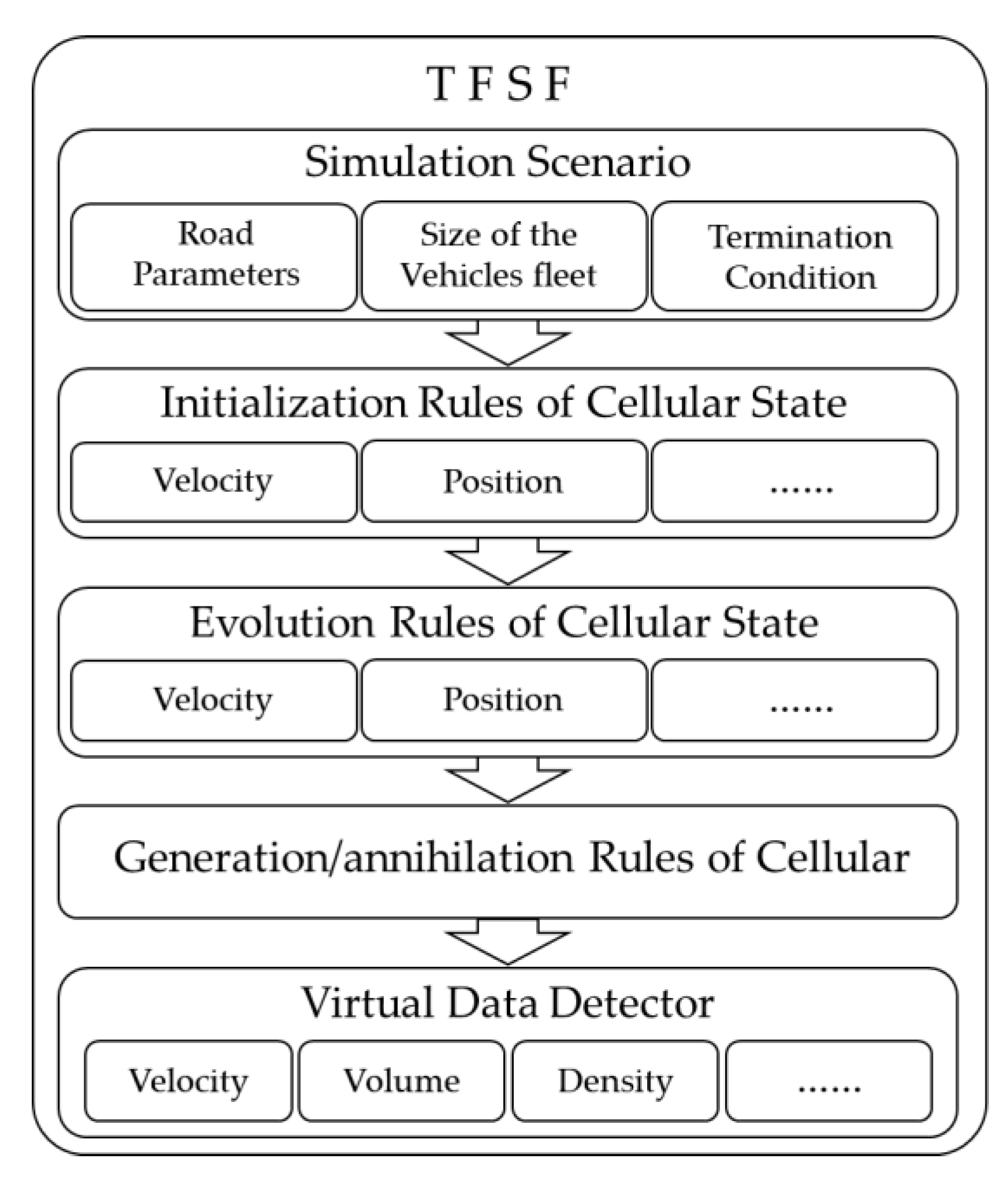
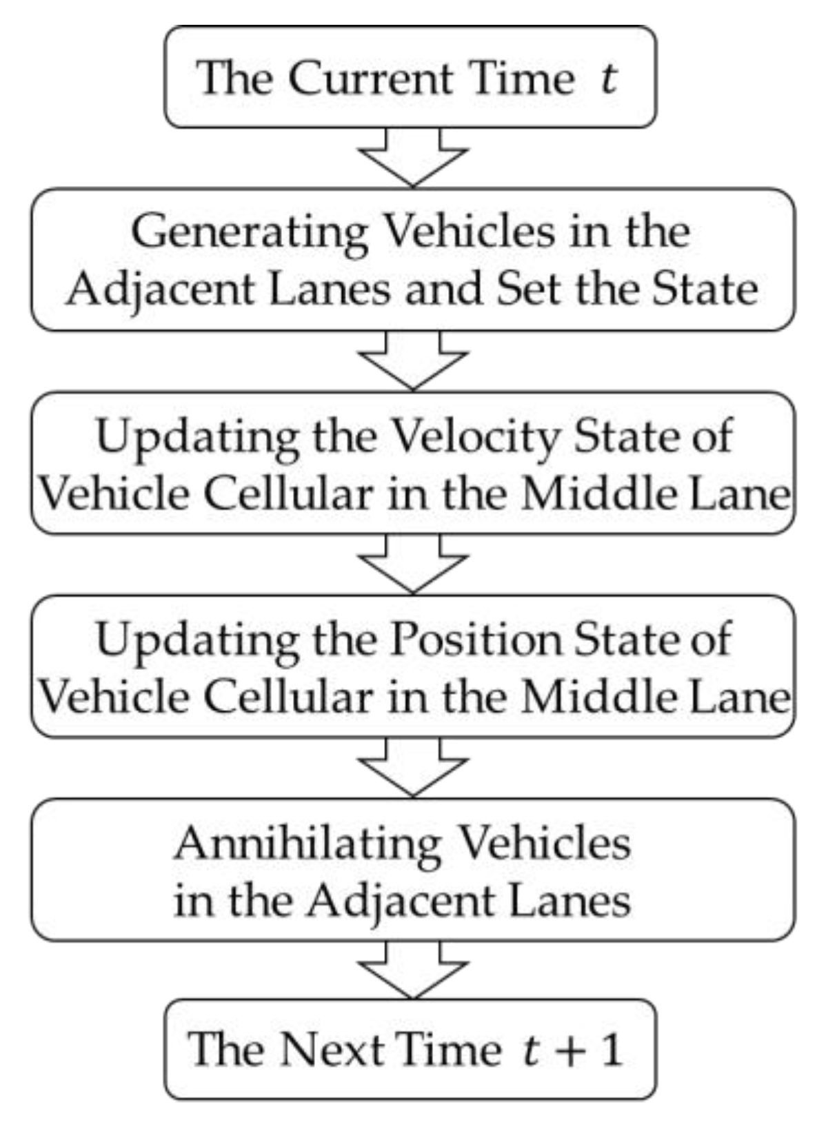
2. Simulation Framework

Car-following behavior is the most basic driving behavior, which is prevalent in the traffic system. As one of the cores of traffic flow theory, car-following models can describe the interaction between the successive vehicles in a detailed way, which are the theoretical basis of macro-characteristics of traffic flow and its simulation. Bando et al. [34] believed that drivers would adjust their car-following behavior according to the distance between their vehicle and the front vehicle, and constructed an optimal velocity (OV) model. (All abbreviations, including the ones in the Abstract, and the corresponding full names are as shown in Table A1 in the Appendix A). Calibrating the OV model with trajectory data, Helbing et al. [35] found that the model would compute unrealistic acceleration/deceleration. To fix this default, Helbing et al. established a generalized force (GF) model with consideration of the negative velocity effect. In the following research, it was found [36] that the GF model could not describe the phenomenon that the object vehicle would not decelerate when the distance between it and its front vehicle was shorter than the safety distance and the front vehicle is much faster than the object vehicle. Based on this, Jiang et al. [37] further considered the positive velocity effect and proposed a full velocity difference (FVD) model. The equation of the FVD model is as follows:
d v n ( t ) d t = a [ V ( Δ x n ) v n ( t ) ] + λ Δ v n
where a is the sensitivity parameter of the driver, V ( Δ x n ) is the optimal velocity function, Δ x n = x n + 1 ( t ) x n ( t ) denotes the headway of two successive vehicles and Δ v n = v n + 1 ( t ) v n ( t ) represents their velocity difference. x n + 1 ( t ) , x n ( t ) , v n + 1 ( t ) and v n ( t ) , respectively, are the position and velocity of the n th vehicle and its front vehicle n + 1 th where t represents time.
The above models are generally referred to as “optimal velocity models”, and the core of these models is the optimal velocity function, which is as follows:
V ( Δ x n ) = v max 2 [ tanh ( Δ x n h c ) + tanh ( h c ) ]
V ( Δ x n ) = V 1 + V 2 tanh [ C 1 ( Δ x n l c ) C 2 ]
where v max is the maximum velocity, h c and l c are the length of the vehicle, V 1 , V 2 , C 1 and C 2 are parameters to be calibrated.
The optimal velocity function has properties including monotonically increasing, existing upper bound, existing inflection point at Δ x n = h c , V ( Δ x n ) 0 when Δ x n 0 and V ( Δ x n ) v max when Δ x n , which enable the function to be able to describe characteristics, such as avoiding collisions, following velocity depending on the distance, driving faster when they can, of drivers’ car-following behavior from a mathematical standpoint. In subsequent studies, the optimal velocity models, especially the FVD model, showed a high performance in simulating car-following behavior in a vehicles fleet and analyzing the stability of the traffic flow. Many extended models were proposed.
However, the optimal velocity models can only reflect the interaction between the object vehicle and its front vehicle, and there are problems existing in directly employing these models to describe drivers’ car-following behavior in the V2X environment. Although there are multiple extended models mentioned in Section 1 with consideration of the impacts exerted by the motion state information of an arbitrary number of preceding vehicles in the current lane, there was no research considering the influence caused by preceding vehicles in the adjacent lanes, of which information is available for the driver in the V2X environment. Based on these, we considered the motion state information of GPV, which consists of the preceding vehicle, the non-neighboring preceding vehicle and the left/right preceding vehicle in the adjacent lanes, and proposed an extended model named the GPV model [33]. The equation of this model is as follows:
d v n ( t ) d t = p { a [ V ( Δ x n ) v n ( t ) ] + λ v n ( t ) } + ( 1 p ) ( v n ¯ v n ( t ) )
where a , λ and p respectively represent the sensitivity of the driver about optimal velocity difference, velocity difference and the difference between the GPV’s average velocity and self-vehicle velocity. v n ¯ is the average velocity of GPV and v n ¯ = ( v n + 1 ( t ) + v n + 2 ( t ) + v l ( t ) + v r ( t ) ) / 4 , where v n + 1 ( t ) , v n + 2 ( t ) , v l ( t ) and v r ( t ) are the velocity of front vehicle, non-neighboring front vehicle, left and right front vehicles in adjacent lanes.
In the GPV model, the optimal velocity function in Equation (3) was employed and the parameters in the function are as shown in Table 1.
Performance of the GPV model in describing drivers’ car-following behavior with consideration of the GPV motion state information in the V2X environment has been confirmed, and the parameters of the model has been calibrated (the calibration results are as shown in Table 2) with the NGSIM dataset in our previous research. And the stability criterion was also obtained through the linear stability analysis, which confirmed the stabilization effect of GPV information on traffic flow. This research as well as other research mentioned above have explored the drivers’ car-following behavior and the stability of traffic flow affected by various information in the V2X environment. However, the quantitative analysis of the traffic flow characteristics is absent in these efforts.
The characteristics of traffic flow are essentially the overall expression of the microscopic car-following behavior of individual vehicles in the system. The macroscopic traffic flow models [38,39,40,41,42,43], which are also known as continuous medium models, are the commonly used approach to explore the impacts of V2X technology on traffic flow in the previous work. In these continuous medium models, vehicles in the system are regarded as a compressible medium, and fluid dynamics as well as other related theories are used to study the traffic flow at the system level. However, these models show a relatively low performance in expressing the differences in macro characteristics of traffic flow caused by the differences in drivers’ micro behavior. Based on this, a simulation framework is combined with the car-following model and the CA for the quantitative analysis of traffic flow characteristics affected by the GPV information in the V2X environment.
As a mesh dynamic model, the CA model is suitable for simulating the space-time evolution process of complex systems and has been widely used in the simulation of traffic flow [44,45,46,47,48,49,50,51,52,53,54,55,56,57,58,59]. Ordinary CA models, as shown in Figure 1, employed in the simulation of traffic flow define the discrete road sections as cellular. In these models, the cellular state contains whether there is or is not a vehicle and other information, and updates according to the pre-set evolution rules.
Research based on discrete CA models could make reappear the evolution of traffic flow and some macroscopic phenomena during the simulation, but the output data are discrete and stepped. Thus, there are some defaults for the discrete CA models in studying traffic flow, especially in the exploration of continuous operation and evolution on the timescale. Although the above problems can be solved to a certain extent by further subdividing the road sections, this approach can obtain approximately continuous data at the cost of consuming massive computing power, which makes the approach not suitable for the simulation of the large-scale transportation system. To solve these problems, Yeldan et al. [60,61,62,63,64,65] defined the vehicles as cellular instead of road sections and proposed the continuous CA model (as shown in Figure 2) for simulating traffic flow.
In the continuous CA model, the vehicles are defined as cellular, and their motion is regarded as the evolution of cellular states, which enables the model to output data continuous on the time scale. However, the evolution rules in the continuous CA models, which have been applied in simulating traffic flow, are relatively simple and, thus, cannot represent the characteristics of drivers’ car-following behavior and directly be used in simulation traffic flow in the V2X environment. Motived by these facts, we define the vehicles as cellular and the velocity as well as position of the vehicles as the cellular state and set the evolution rules based on the car-following model. Based on this, a traffic flow simulation framework (TFSF) for the research on traffic flow characteristics is constructed. The basic structure of the TFSF can be seen in Figure 3.
In this work, the evolution rules of the cellular state are set based on the GPV model to explore the operating characteristics of traffic flow affected by GPV information in the V2X environment.
Rules in the TFSF are set as follows:
Initialization Rules of Cellular State
In the TFSF, the vehicles are defined as cellular, and the state of each cellular state contains the position and velocity of the corresponding vehicle, i.e., S n = [ x n ( t ) , v n ( t ) ] . The initialization rules of the cellular state are as follows:
(1) Position. At the initial time, there are a total of N vehicles on the road with a length of L . Assigning the same motion area l for all vehicles, and the initial position of the n th ( n = 1 , 2 , , N ) vehicle x n ( 0 ) , which is defined as the distance between the vehicle head and the starting line of the road, this can be given as
x n ( 0 ) ~ N ( n d l + ( h c d l ) / 2 , ( d l h c ) 2 / 36 )
where d l = L / N is the length of the motion area l , and h c is the length of the vehicle.
According to the properties of normal distribution, it is necessary to set constraints to avoid the “overlapping” phenomenon, which means the two successive vehicles overlap in space. The constraints are as follows:
i f x m ( 0 ) > m d l
t h e n x m ( 0 ) = m d l
i f x m ( 0 ) < ( m 1 ) d l + h c
t h e n x m ( 0 ) = ( m 1 ) d l + h c
where m = 1 , 2 , , N .
(2) Velocity. According to the NGSIM data, the initial velocity of the vehicle is set as
v n ( 0 ) = min { max [ r 1 v max , v min ] , v d n }
where r 1 is a random number and r 1 ( 0 , 1 ] , v max and v min are, respectively, the upper and lower limit of velocity in the simulation, v d n is the safety limit of velocity to avoid collision, and its value is equal to the headway between the n th vehicle and its front vehicle, i.e., d n ( t ) = x n + 1 ( t ) x n ( t ) h c .
Evolution Rules of Cellular State
For each simulation step, the state of each vehicle cell in the system is updated simultaneously according to the following rules:
(1) Velocity. The velocity of the n th vehicle at the next time t + 1 can be given as
v n ( t + 1 ) = min { v max , v d n , max [ 0 , v n ( t ) + a n ( t ) ] }
where v n ( t + 1 ) and v n ( t ) are, respectively, the velocity of the n th vehicle at the time t and the next time t + 1 , and a n ( t ) is the acceleration of the n th vehicle at the time t , which can be determined according to Equation (4).
(2). Position. The position of the n th vehicle at the next time t + 1 is
x n ( t + 1 ) = x n ( t ) + v n ( t + 1 )
where r 2 is a random number and r 2 ~ N ( 0.5 , 0.0225 ) , and v m t is the maximum velocity of all vehicles at the time t .
It is very rare that two vehicles in the two adjacent lanes side by side are driving at the same velocity. Due to this, a random noise is added to the state of the cell when the generated left and right front vehicles have the same velocity and the same position. Then, the velocity of the n th vehicle’s left front vehicle at the time t is
v r ( t ) = v min + r 3 ( v max v min )
i f v r ( t ) = v l ( t )
t h e n v r ( t ) = v r ( t ) + r 4
where r 3 and r 4 are random numbers, r 3 ~ N ( 0.5 , 0.0225 ) and r 4 ~ N ( 0 , 1 ) .
(2) Position. The position of the n th vehicle’s left front vehicle at the time t is a random number as
x l ( t ) = r a n d [ x n , x n + 1 ]
That of the right front vehicle of the n th vehicle at the time t is
x l ( t ) = r a n d [ x n , x n + 1 ]
i f x r ( t ) = x l ( t )
t h e n x r ( t ) = x r ( t ) + r 5
where r 5 is a random number and r 5 ~ N ( 0 , 1 ) .
To sum up, the evolution process of the cellular state can be seen in Figure 4.
Initialization and Annihilation Rules of Cellular States
The periodic boundary condition is used in this work, which means the cellular state annihilates when the corresponding vehicle drives out of the road and a cellular state generates in the beginning of the road with the same state at the same time. Among all object vehicles in the middle lane, the vehicle group, which form the GPV, of the N th and the N 1 th vehicle, respectively, lacks the preceding vehicle and the non-neighboring preceding vehicle. According to the properties of the periodic boundary condition, the first vehicle can be regarded as the preceding vehicle of the N th vehicle and the non-neighboring preceding vehicle of the N 1 th vehicle, and the second vehicle can be regarded as the non-neighboring preceding vehicle of the N 1 th vehicle.

3. Simulation

The TFSF used in this section is based on the GPV model that has been verified. Thus, it is unnecessary to carry out the verification on the performance of the TFSF in describing drivers’ car-following behavior affected by the GPV information in the V2X environment. All simulation conducted in this section was accomplished with the MATLAB software (Version 9.6).

3.1. Setting of the Simulation Scenario

According to the data measured in the field and the previous research [33,66], the length of the road and the vehicle are respectively set as L = 1500 m and h c = 5 m. The velocity limits are set as v max = 30 m/s and v min = 8 m/s. The acceleration limits are set as a max = 3 m/s2 and a min = 4 m/s2. The total time of the simulation is T = 3000 s. Letting N represent the total number of the vehicles on the road, one can obtain
{ v f = v ¯ k = L / N q = v f k
where v f is the operating velocity of traffic flow, and v ¯ is the average velocity of all object vehicles. k is the density of vehicles on the road. q is the volume of traffic flow.

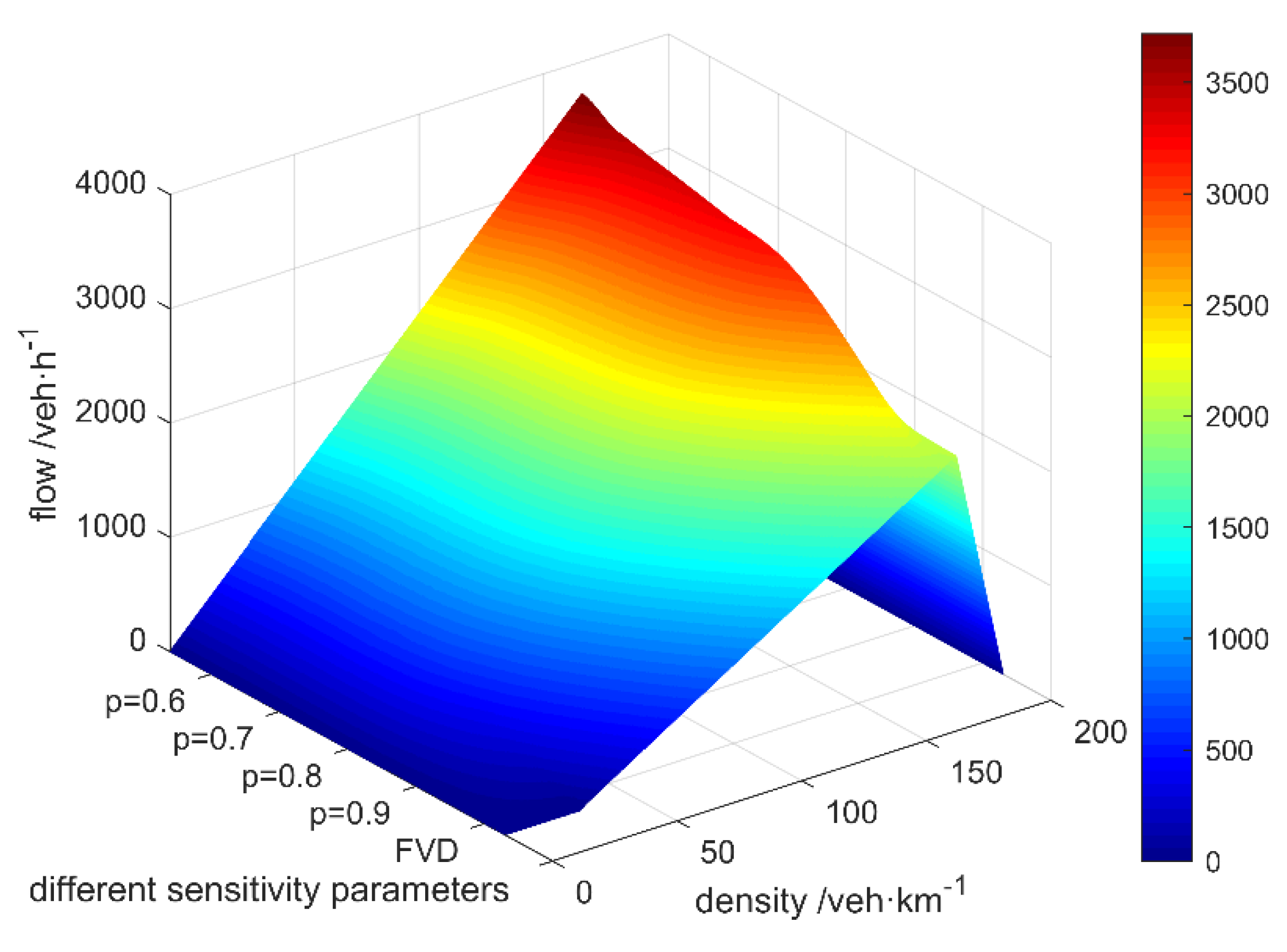
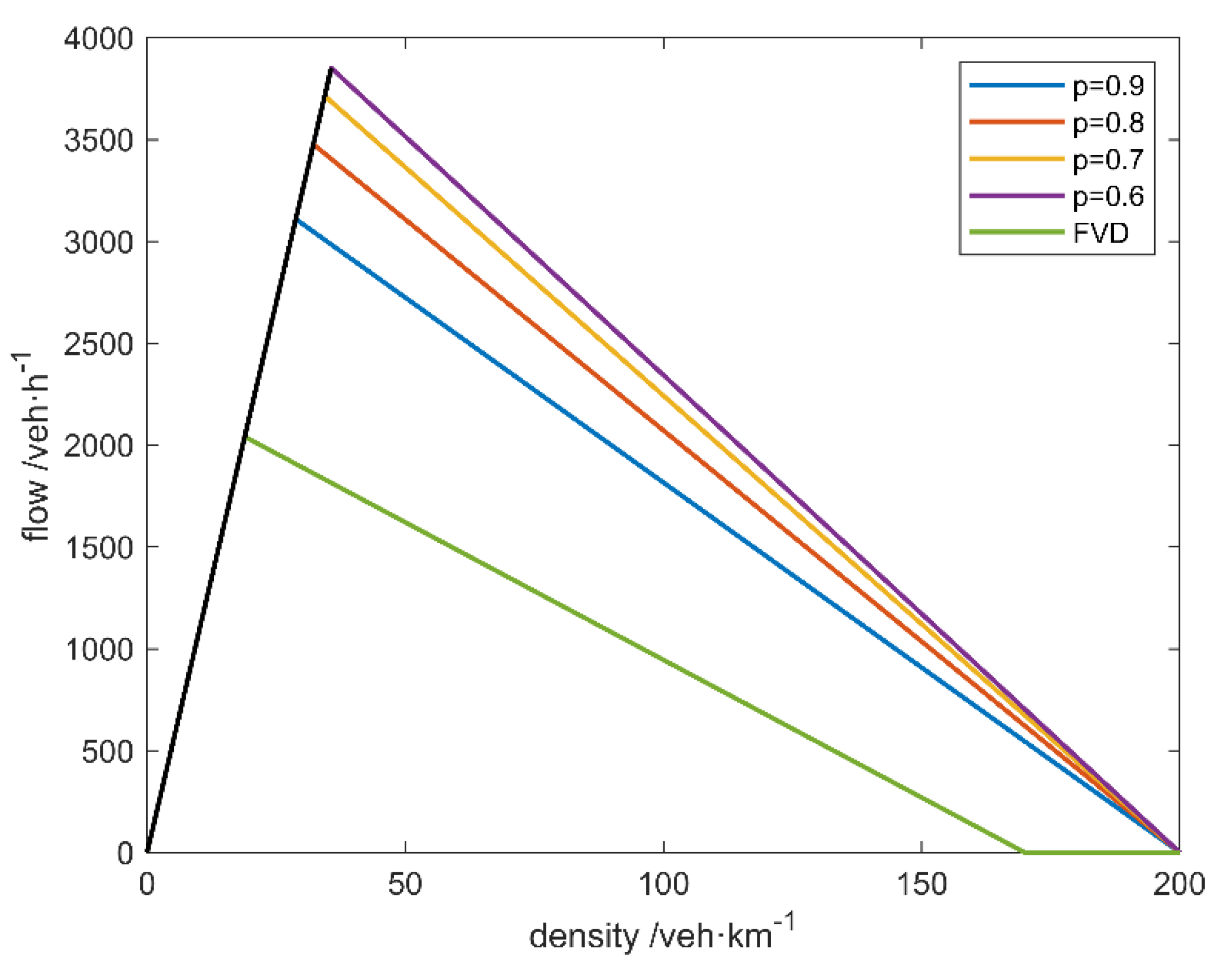
3.2. The Simulation of Traffic Flow

To explore the impacts of GPV information on traffic flow under different levels of drivers’ attention to the information, the sensitivity parameter p is respectively set as 0.9, 0.8, 0.7 and 0.6. The FVD model is employed to represent the unconnected environment for comparison. The calibrated values of the corresponding parameters can be seen in Table 1 and Table 2. With the simulation of the traffic flow affected by the GPV information in the V2X environment, a volume–density surface can be obtained as shown in Figure 5.
As shown in Figure 5, the GPV information in the V2X environment has a significant positive influence on the operation of traffic flow. In the V2X environment, the maximum volumes of the traffic flow affected by the GPV information with a different sensitivity parameter p are as shown in Table 3.
From Table 3, one can obtain that the maximal volume of traffic flow affected by the GPV information in the V2X environment is significantly increased, and the rate of the increase can reach up to 88.73% compared with the unconnected environment, in which the maximum volume of the traffic flow is 2040.96 veh∙h−1 under the same condition. To further explore the positive effect of the GPV information on the traffic flow in the V2X environment, extra simulation is carried out, and the fundamental diagram represented by the volume–density relationship is obtained, which can be seen in Figure 6.
From Figure 6, one can obtain that compared with the unconnected environment, the traffic flow in the V2X environment can maintain the free-flow state under the condition of a higher density of vehicles. The traffic flow in the V2X environment can operate with a higher value of volume and velocity, which is expressed by the derivative value at the corresponding points, under the same density of vehicles after breaking away from the free-flow state. Besides, the jamming density in the V2X environment is much higher than that in the unconnected environment.
To reflect the impacts of the GPV information on the operating velocity of traffic flow, the velocity–density surface and the corresponding velocity–density curves are obtained and can be seen in Figure 7 and Figure 8.
As shown in Figure 7 and Figure 8, the traffic flow can only maintain the free-flow state within the density of 18.91 veh/km in the unconnected environment, and the traffic flow affected by the GPV information can maintain the free-flow state within the density up to 35.67 veh/km in the V2X environment. The breaking values of density, which mean the traffic flow cannot maintain a free-flow state when the density is higher than this value under the corresponding condition, affected by the GPV information with different values of sensitivity parameter p in the V2X environment, are as shown in Table 4.
After breaking away from the free-flow state, the traffic flow affected by the GPV information in the V2X environment would operate with higher values of velocity and volume than those in the unconnected environment. The jamming density of traffic flow in the unconnected environment is 170.00 veh∙km−1. By contrast, the jamming density of traffic flow affected by the GPV information in the V2X environment can reach up to 197.79 veh∙km−1, which means the increase is up to 16.35%, under the same condition. These results are consistent with the fundamental diagram in the above contents. It is worth noting that there is a phenomenon of a “steep drop” of operating velocity after the traffic flow breaks away from the free-flow state in the unconnected environment represented by the FVD model. This phenomenon may be caused by the increase of density, which usually means an increase of headway and decrease of the velocity when the traffic flow breaks away from the free-flow state. These changes in density and velocity can be regarded as a disturbance, to a certain extent. When the changes happen, it can be regarded as a disturbance that emerges in the traffic flow and then propagates in the vehicle fleet, which eventually causes the “steep drop” of the operating velocity of the traffic flow.

3.3. Simulation on the Impacts of Disturbance on Traffic Flow

In the previous section, the traffic flow affected by the GPV information in the V2X environment was simulated, and the operating characteristics of the traffic flow were explored. With the simulation, one can obtain that the traffic flow affected by the GPV information could maintain the free-flow state with higher density and operate with higher velocity when it breaks away from the free-flow state. To reveal the operating characteristics of traffic flow affected by the GPV information in the V2X environment, the disturbance was not considered in the previous simulation. However, the disturbance is not rare in the realistic traffic system. For instance, when a vehicle in the system changes its velocity, the headway between the vehicle and its preceding as well as its rear vehicle, a disturbance emerges in the system and will affect the operating of traffic flow. Based on this, the impacts of disturbance on the traffic flow affected by the GPV information in the V2X environment are simulated and explored in this section. Parameters of the simulation scenario are set as: p = 0.769 , L = 1000 m and N = 50 . When t = 1000 s, a disturbance with the scale of 4 m/s is exerted in the traffic flow, and the simulation continues. The FVD model is employed to represent the unconnected environment for comparison. The propagation of disturbance has been discussed in our previous work [33], and the attention is attached to the impacts of the disturbance on traffic flow in this research. The simulation results are as shown in Figure 9 and Figure 10.
As shown in Figure 9a and Figure 10a, the traffic flow in the two kinds of environment are all at a free-flow and equilibrium state before exerting the disturbance. Compared with the unconnected environment, the traffic flow affected by the GPV information is operating with the velocity 30.73 km∙h−1 in the V2X environment. By contrast, the traffic flow is operating with the velocity 28.47 km∙h−1 in the unconnected environment.
From Figure 9b and Figure 10b, one can obtain that the time for the traffic flow in the unconnected environment returns to an equilibrium and stable state is 540 s, and that for the traffic flow affected by the GPV information in the V2X environment it is 300 s. The improvement in the time for traffic flow to return to an equilibrium and stable state is up to 44.44%. Besides, the deviation of operation of the traffic flow affected by the GPV information from the state before the exerting of disturbance is slighter than that of the traffic flow in the unconnected environment. The deviation in the V2X environment is 6.38%, which is represented by the velocity deviation, and the improvement on the deviation is up to 25.27%.

4. Discussion

The macroscopic characteristics of traffic flow are essentially the overall expression of the microscopic behavior of individual vehicles in the system. The application of the V2X technology to the traffic system significantly enhanced the information perception ability of drivers and, thus, affects their car-following behavior, which will cause differences in the characteristics of traffic flow. The impacts of various connected information on drivers’ car-following behavior and traffic flow have been explored in the previous research [19,20,21,22,23,24,25,26,27,28,29,30,31,32], and the car-following behavior as well as the stability characteristics of traffic flow affected by various connected information have been studied. However, quantitative analysis of the operating characteristics of traffic flow affected by the GPV information in the V2X environment is still absent. The influence of connected technology on the traffic system has attracted more and more attention, and many achievements have been reported [38,39,40,41,42,43,67,68,69,70,71,72,73,74]. The impacts of V2X and other connected technologies on the traffic system have been discussed based on various theories and methods in the previous research. However, there are some limitations for these efforts to answer the question of the impacts of GPV information on traffic flow in a quantitative way, including the continuous medium models [38,39,40,41,42,43] as well as its limitations mentioned in the previous section. In addition to the continuous medium models, the research [70,71,72,73,74] based on the Intelligent Driver Model as well as other related methods is another research hotpot in the field. These efforts focus on the impacts of the cooperative adaptive cruise control (CACC) system equipped on the traffic flow, and the impacts of various connected information, especially the GPV information, on the traffic flow are not explored in those efforts. Moreover, there are many difficulties in employing the models as well as the methods used in these efforts to explore the impacts of various information on the traffic flow. On the one hand, the CACC system is a longitudinal driving assistance system that assists the driver to manipulate the vehicle to follow the preceding vehicle (fleet) in the current lane. The preceding vehicles in the adjacent lanes are not considered in the system, with the result that the corresponding efforts cannot be used in the exploration on the impacts of GPV information on traffic flow. On the other hand, as a driving assistance system, the CACC system can automatically respond to the motion of the preceding vehicles in the current lane, with the result that the corresponding efforts cannot be used in the exploration of the impacts of difference attention degree of the connected information on traffic flow. In summary, the previous achievements are not suitable for answering the question of the impacts of GPV information on traffic flow in the V2X environment.
Motivated by this, we proposed a simulation framework (the TFSF) based on the car-following model and the CA, then employed the TFSF in the quantitative analysis of traffic flow affected by the GPV information in the V2X environment. The research results suggest that there is a significant positive influence of the GPV information on the traffic flow in the V2X environment. As shown in Figure 5, Figure 6, Figure 7 and Figure 8, the traffic flow affected by the GPV information could maintain the free-flow state under the condition of a much higher density of vehicles, and the maximal volume of the traffic flow at the free-flow state is much higher than that in the unconnected environment. The value of the operating velocity as well as the jamming density is higher than that in the unconnected environment when the traffic flow breaks away from the free-flow state. These positive effects of the GPV information are enhanced with more drivers’ attention attached to the GPV information. It is noteworthy that the enhancement rate of these positive effects, as shown in Table 3 and Table 4, is getting lower as drivers pay more attention to the GPV information. This is consistent with the characteristics that the driver pays attention to the GPV information rather than focusing on the information when he/she is in the car-following state. The impacts of disturbance on the traffic flow affected by the GPV information in the V2X environment were explored with simulation based on the TFSF. The results reveal that the traffic flow operates with higher velocity than that in the unconnected environment before exerting the disturbance, which is consist with the above results. After exerting the disturbance, the time for the traffic flow affected by the GPV information to return to an equilibrium and stable state is shorter than that in the unconnected environment, and the traffic flow affected by the GPV information could operate with higher velocity when returned to an equilibrium and stable state. The deviation of the operation state of the traffic flow affected by the GPV information in the V2X environment is smaller than that in the unconnected environment. These results confirm the positive effects of the GPV information on the traffic flow in the V2X environment.
The TFSF proposed in this work is essentially an extended one-dimension three-lane CA model with good expansibility, which ensures the TFSF is suitable for simulating the traffic flow affected by various information in the V2X environment with some adjustment of the parameters or rules in it. As shown in Figure 3, the expansibility of TFSF means that the TFSF can be used in simulating the operation characteristics of traffic flow affected by various information in the V2X environment by setting the parameters about the scenario as well as the vehicle fleet, the initialization and evolution rules of cellular states and the generation as well as annihilation rules of cellular states according to the research needs. Adjusting the parameters about the scenario and the vehicle fleet can make the TFSF suitable for simulating the traffic flow in various systems with different scales. Changing the initialization and evolution rules of the cellular state can give TFSF the ability to simulate the traffic flow affected by the various connected information. For instance, setting Equation (11) of the evolution rules of the cellular state according to the calculation formula given in [28] can give TFSF the ability to simulate the traffic flow affected by the average velocity information of the arbitrary number of preceding vehicles in the current lane. The TFSF proposed in this work can be utilized in simulating the traffic flow under the open boundary condition by altering the generation and annihilation rules of cellular states.
This work focuses on the impacts of connected technologies on the transportation system. By means of numerical simulation, the positive effects of the GPV information on the operation characteristics of traffic flow in the V2X environment and the impacts of different degrees of drivers’ attention to the connected information on these positive effects were quantitatively analyzed, which can provide a reference for the design and management of the transportation system with new connected technologies. An approach to link the macro-characteristics of traffic flow to the micro-characteristics of driving behavior was proposed, and it can be employed in exploring the operating characteristics of traffic flow in different development stages of the V2X technology.
The TFSF proposed in this work as well as the research results can provide the theoretical basis and method reference for further research on the characteristics of traffic flow in the V2X environment. However, there are some shortcomings in this research. For instance, the TFSF employed to simulate the traffic flow affected by the GPV information is essentially an extended one-dimension three-lane CA model to ensure the integrity of the vehicle group that constitutes the GPV. However, the generation as well as annihilation rules of cellular states and the initialization as well as the evolution rules of cellular states are relatively simple and cannot perfectly represent the moving characteristics of the left/right preceding vehicle in the realistic transportation system, which we look forward to improving in our future work.

5. Conclusions

A simulation framework based on the car-following model and CA was proposed in this work and then employed to simulate the traffic flow affected by the GPV information in the V2X environment. With the simulation, operation characteristics of the traffic flow were explored quantitatively. The research results suggest that the operation of the traffic flow has been effectively improved with the GPV information, and the improvement degree is up to 88.73%, which is calculated by the maximal volume of traffic flow. It is confirmed that the application of the V2X and other connected technologies has positive impacts on traffic flow and can effectively improve transportation efficiency.

Author Contributions

Writing—original draft, J.H.; Writing—review & editing, X.W.; Software, J.H., H.S. and J.Z.; Validation, J.H., C.B. and J.Z.; Visualization, J.H. and G.W.; Funding acquisition, X.W.; Project administration, X.W.; Resources, X.W.; Supervision, X.W.; Formal analysis, C.B.; Methodology, C.B.; Investigation, H.S. All authors have read and agreed to the published version of the manuscript.

Funding

This study was funded by the National Key Research and Development Project (Grant No.2018YFB1601500), the Natural Science Foundation of Shandong Province (Grant No. ZR2020MF082), the Qingdao Top Talent Program of Entrepreneurship and Innovation (Grant No.19-3-2-11-zhc) and the Foundation of Shandong Intelligent Green Manufacturing Technology and Equipment Collaborative Innovation Center (Grant No. IGSD-2020-012).

Data Availability Statement

Not Applicable, the study does not report any data.

Conflicts of Interest

The authors declare no conflict of interest.

Appendix A

All abbreviations used in this article and the corresponding full names are as shown in Table A1.
Table A1. All abbreviations and the corresponding full names.
AbbreviationsFull Name
V2Xvehicles to everything
GPVgeneralized preceding vehicles
CAcellular automata
OVoptimal velocity
GFgeneralized force
FVDfull velocity difference
TFSFtraffic flow simulation framework
CACCcooperative adaptive cruise control

References

  1. Kuutti, S.; Fallah, S.; Katsaros, K.; Dianati, M.; Mccullough, F.; Mouzakitis, A. A Survey of the State-of-the-Art Localization Techniques and Their Potentials for Autonomous Vehicle Applications. IEEE Internet Things J. 2018, 5, 829–846. [Google Scholar] [CrossRef]
  2. Haider, A.; Hwang, S.H. Adaptive Transmit Power Control Algorithm for Sensing-Based Semi-Persistent Scheduling in C-V2X Mode 4 Communication. Electronics 2019, 8, 846. [Google Scholar] [CrossRef] [Green Version]
  3. Mannoni, V.; Berg, V.; Sesia, S.; Perraud, E. A Comparison of the V2X Communication Systems: ITS-G5 and C-V2X. In Proceedings of the 2019 IEEE 89th Vehicular Technology Conference (VTC2019-Spring), Kuala Lumpur, Malaysia, 28 April–1 May 2019; pp. 1–5. [Google Scholar]
  4. Naik, G.; Choudhury, B.; Park, J.-M. IEEE 802.11bd & 5G NR V2X: Evolution of Radio Access Technologies for V2X Communications. IEEE Access 2019, 7, 70169–70184. [Google Scholar] [CrossRef]
  5. Chen, S.; Hu, J.; Shi, Y.; Zhao, L.; Li, W. A Vision of C-V2X: Technologies, Field Testing, and Challenges with Chinese Development. IEEE Internet Things J. 2020, 7, 3872–3881. [Google Scholar] [CrossRef] [Green Version]
  6. Qi, W.; Landfeldt, B.; Song, Q.; Guo, L.; Jamalipour, A. Traffic Differentiated Clustering Routing in DSRC and C-V2X Hybrid Vehicular Networks. IEEE Trans. Veh. Technol. 2020, 69, 7723–7734. [Google Scholar] [CrossRef] [Green Version]
  7. Romeo, F.; Campolo, C.; Molinaro, A.; Berthet, A.O. DENM Repetitions to Enhance Reliability of the Autonomous Mode in NR V2X Sidelink. In Proceedings of the 2020 IEEE 91st Vehicular Technology Conference (VTC2020-Spring), Antwerp, Belgium, 25–28 May 2020; pp. 1–5. [Google Scholar]
  8. Tang, F.; Kawamot, Y.; Kato, N.; Liu, J. Future Intelligent and Secure Vehicular Network Toward 6G: Machine-Learning Approaches. Proc. IEEE 2020, 108, 292–307. [Google Scholar] [CrossRef]
  9. Zadobrischi, E.; Dimian, M. Vehicular Communications Utility in Road Safety Applications: A Step toward Self-Aware Intelligent Traffic Systems. Symmetry 2021, 13, 438. [Google Scholar] [CrossRef]
  10. Li, Y.; Wang, H.; Wang, W.; Xing, L.; Liu, S.; Wei, X. Evaluation of the Impacts of Cooperative Adaptive Cruise Control on Reducing Rear-End Collision Risks on Freeways. Accid. Anal. Prev. 2017, 98, 87–95. [Google Scholar] [CrossRef]
  11. Rios-Torres, J.; Malikopoulos, A.A. A Survey on the Coordination of Connected and Automated Vehicles at Intersections and Merging at Highway On-Ramps. IEEE Trans. Intell. Transp. Syst. 2017, 18, 1066–1077. [Google Scholar] [CrossRef]
  12. Stern, R.E.; Cui, S.; Delle Monache, M.L.; Bhadani, R.; Bunting, M.; Churchill, M.; Hamilton, N.; Haulcy, R.; Pohlmann, H.; Wu, F.; et al. Dissipation of Stop-and-Go Waves via Control of Autonomous Vehicles: Field Experiments. Transp. Res. Part C Emerg. Technol. 2018, 89, 205–221. [Google Scholar] [CrossRef] [Green Version]
  13. Papadoulis, A.; Quddus, M.; Imprialou, M. Evaluating the Safety Impact of Connected and Autonomous Vehicles on Motorways. Accid. Anal. Prev. 2019, 124, 12–22. [Google Scholar] [CrossRef] [Green Version]
  14. Ye, L.; Yamamoto, T. Evaluating the Impact of Connected and Autonomous Vehicles on Traffic Safety. Phys. Stat. Mech. ITS Appl. 2019, 526. [Google Scholar] [CrossRef]
  15. Zadobrischi, E.; Cosovanu, L.-M.; Dimian, M. Traffic Flow Density Model and Dynamic Traffic Congestion Model Simulation Based on Practice Case with Vehicle Network and System Traffic Intelligent Communication. Symmetry 2020, 12, 1172. [Google Scholar] [CrossRef]
  16. Farah, H.; Koutsopoulos, H.N. Do Cooperative Systems Make Drivers’ Car-Following Behavior Safer? Transp. Res. Part C Emerg. Technol. 2014, 41, 61–72. [Google Scholar] [CrossRef]
  17. Li, X.; Cui, J.; An, S.; Parsafard, M. Stop-and-Go Traffic Analysis: Theoretical Properties, Environmental Impacts and Oscillation Mitigation. Transp. Res. Part B Methodol. 2014, 70, 319–339. [Google Scholar] [CrossRef]
  18. Jia, D.; Ngoduy, D. Enhanced Cooperative Car-Following Traffic Model with the Combination of V2V and V2I Communication. Transp. Res. Part B Methodol. 2016, 90, 172–191. [Google Scholar] [CrossRef]
  19. Nagatani, T. Stabilization and Enhancement of Traffic Flow by the Next-Nearest-Neighbor Interaction. Phys. Rev. E 1999, 60, 6395–6401. [Google Scholar] [CrossRef] [Green Version]
  20. Lenz, H.; Wagner, C.K.; Sollacher, R. Multi-Anticipative Car-Following Model. Eur. Phys. J. B 1999, 7, 331–335. [Google Scholar] [CrossRef]
  21. Ge, H.X.; Dai, S.Q.; Dong, L.Y.; Xue, Y. Stabilization Effect of Traffic Flow in an Extended Car-Following Model Based on an Intelligent Transportation System Application. Phys. Rev. E 2004, 70, 066134. [Google Scholar] [CrossRef]
  22. Li, Z.-P.; Liu, Y.-C. Analysis of Stability and Density Waves of Traffic Flow Model in an ITS Environment. Eur. Phys. J. B 2006, 53, 367–374. [Google Scholar] [CrossRef]
  23. Peng, G.H.; Sun, D.H. A Dynamical Model of Car-Following with the Consideration of the Multiple Information of Preceding Cars. Phys. Lett. A 2010, 374, 1694–1698. [Google Scholar] [CrossRef]
  24. Li, Y.; Sun, D.; Liu, W.; Zhang, M.; Zhao, M.; Liao, X.; Tang, L. Erratum to: Modeling and Simulation for Microscopic Traffic Flow Based on Multiple Headway, Velocity and Acceleration Difference. Nonlinear Dyn. 2011, 66, 845. [Google Scholar] [CrossRef] [Green Version]
  25. Hu, Y.; Ma, T.; Chen, J. An Extended Multi-Anticipative Delay Model of Traffic Flow. Commun. Nonlinear Sci. Numer. Simul. 2014, 19, 3128–3135. [Google Scholar] [CrossRef]
  26. Chen, J.; Liu, R.; Ngoduy, D.; Shi, Z. A New Multi-Anticipative Car-Following Model with Consideration of the Desired Following Distance. Nonlinear Dyn. 2016, 85, 2705–2717. [Google Scholar] [CrossRef]
  27. Guo, L.; Zhao, X.; Yu, S.; Li, X.; Shi, Z. An Improved Car-Following Model with Multiple Preceding Cars’ Velocity Fluctuation Feedback. Phys. Stat. Mech. Its Appl. 2017, 471, 436–444. [Google Scholar] [CrossRef]
  28. Sun, D.; Kang, Y.; Yang, S. A Novel Car Following Model Considering Average Speed of Preceding Vehicles Group. Phys. Stat. Mech. Its Appl. 2015, 436, 103–109. [Google Scholar] [CrossRef]
  29. Kuang, H.; Xu, Z.-P.; Li, X.-L.; Lo, S.-M. An Extended Car-Following Model Accounting for the Average Headway Effect in Intelligent Transportation System. Phys. Stat. Mech. Its Appl. 2017, 471, 778–787. [Google Scholar] [CrossRef]
  30. Guo, Y.; Xue, Y.; Shi, Y.; Wei, F.; Lü, L.; He, H. Mean-Field Velocity Difference Model Considering the Average Effect of Multi-Vehicle Interaction. Commun. Nonlinear Sci. Numer. Simul. 2018, 59, 553–564. [Google Scholar] [CrossRef]
  31. Wen-Xing, Z.; Li-Dong, Z. A New Car-Following Model for Autonomous Vehicles Flow with Mean Expected Velocity Field. Phys. Stat. Mech. Its Appl. 2018, 492, 2154–2165. [Google Scholar] [CrossRef]
  32. Kuang, H.; Wang, M.-T.; Lu, F.-H.; Bai, K.-Z.; Li, X.-L. An Extended Car-Following Model Considering Multi-Anticipative Average Velocity Effect under V2V Environment. Phys. Stat. Mech. Its Appl. 2019, 527, 121268. [Google Scholar] [CrossRef]
  33. Han, J.; Zhang, J.; Wang, X.; Liu, Y.; Wang, Q.; Zhong, F. An Extended Car-Following Model Considering Generalized Preceding Vehicles in V2X Environment. Future Internet 2020, 12, 216. [Google Scholar] [CrossRef]
  34. Bando, M.; Hasebe, K.; Nakayama, A.; Shibata, A.; Sugiyama, Y. Dynamical Model of Traffic Congestion and Numerical Simulation. Phys. Rev. E 1995, 51, 1035–1042. [Google Scholar] [CrossRef] [PubMed]
  35. Helbing, D.; Tilch, B. Generalized Force Model of Traffic Dynamics. Phys. Rev. E 1998, 58, 133–138. [Google Scholar] [CrossRef] [Green Version]
  36. Treiber, M.; Hennecke, A.; Helbing, D. Derivation, Properties, and Simulation of a Gas-Kinetic-Based, Nonlocal Traffic Model. Phys. Rev. E 1999, 59, 239–253. [Google Scholar] [CrossRef] [Green Version]
  37. Jiang, R.; Wu, Q.; Zhu, Z. Full Velocity Difference Model for a Car-Following Theory. Phys. Rev. E 2001, 64, 017101. [Google Scholar] [CrossRef] [Green Version]
  38. Yi, J.; Horowitz, R. Macroscopic Traffic Flow Propagation Stability for Adaptive Cruise Controlled Vehicles. Transp. Res. Part C Emerg. Technol. 2006, 14, 81–95. [Google Scholar] [CrossRef]
  39. Ngoduy, D. Application of Gas-Kinetic Theory to Modelling Mixed Traffic of Manual and ACC Vehicles. Transportmetrica 2012, 8, 43–60. [Google Scholar] [CrossRef]
  40. Ngoduy, D. Instability of Cooperative Adaptive Cruise Control Traffic Flow: A Macroscopic Approach. Commun. Nonlinear Sci. Numer. Simul. 2013, 18, 2838–2851. [Google Scholar] [CrossRef]
  41. Ngoduy, D. Platoon-Based Macroscopic Model for Intelligent Traffic Flow. Transp. B Transp. Dyn. 2013, 1, 153–169. [Google Scholar] [CrossRef]
  42. Ngoduy, D.; Jia, D. Multi Anticipative Bidirectional Macroscopic Traffic Model Considering Cooperative Driving Strategy. Transp. B Transp. Dyn. 2017, 5, 96–110. [Google Scholar] [CrossRef]
  43. Delis, A.I.; Nikolos, I.K.; Papageorgiou, M. A Macroscopic Multi-Lane Traffic Flow Model for ACC/CACC Traffic Dynamics. Transp. Res. Rec. 2018, 2672, 178–192. [Google Scholar] [CrossRef]
  44. Wolfram, S. Statistical Mechanics of Cellular Automata. Rev. Mod. Phys. 1983, 55, 601–644. [Google Scholar] [CrossRef]
  45. Cremer, M.; Ludwig, J. A Fast Simulation Model for Traffic Flow on the Basis of Boolean Operations. Math. Comput. Simul. 1986, 28, 297–303. [Google Scholar] [CrossRef]
  46. Nagel, K.; Schreckenberg, M. A Cellular Automaton Model for Freeway Traffic. J. Phys. I 1992, 2, 2221–2229. [Google Scholar] [CrossRef]
  47. Biham, O.; Middleton, A.A.; Levine, D. Self-Organization and a Dynamical Transition in Traffic-Flow Models. Phys. Rev. A 1992, 46, R6124–R6127. [Google Scholar] [CrossRef] [PubMed] [Green Version]
  48. Takayasu, M.; Takayasu, H. 1/f noise in a traffic model. Fractals 1993, 1, 860–866. [Google Scholar] [CrossRef]
  49. Nagatani, T. Self-Organization and Phase Transition in Traffic-Flow Model of a Two-Lane Roadway. J. Phys. Math. Gen. 1993, 26, L781–L787. [Google Scholar] [CrossRef]
  50. Fukui, M.; Ishibashi, Y. Traffic Flow in 1D Cellular Automaton Model Including Cars Moving with High Speed. J. Phys. Soc. Jpn. 1996, 65, 1868–1870. [Google Scholar] [CrossRef]
  51. Rickert, M.; Nagel, K.; Schreckenberg, M.; Latour, A. Two Lane Traffic Simulations Using Cellular Automata. Phys. Stat. Mech. Its Appl. 1996, 231, 534–550. [Google Scholar] [CrossRef] [Green Version]
  52. Knospe, W.; Santen, L.; Schadschneider, A.; Schreckenberg, M. Towards a Realistic Microscopic Description of Highway Traffic. J. Phys. Math. Gen. 2000, 33, L477. [Google Scholar] [CrossRef]
  53. Pedersen, M.; Ruhoff, P.T. Entry Ramps in the Nagel-Schreckenberg Model. Phys. Rev. E Stat. Nonlin. Soft Matter Phys. 2002, 65, 056705. [Google Scholar] [CrossRef]
  54. Bham, G.H.; Benekohal, R.F. A High Fidelity Traffic Simulation Model Based on Cellular Automata and Car-Following Concepts. Transp. Res. Part C Emerg. Technol. 2004, 12, 1–32. [Google Scholar] [CrossRef]
  55. He, Y.; Yao, D.; Zhang, Y.; Pei, X.; Li, L. Cellular Automaton Model for Bidirectional Traffic under Condition of Intelligent Vehicle Infrastructure Cooperative Systems. In Proceedings of the 2016 IEEE International Conference on Vehicular Electronics and Safety (ICVES), Beijing, China, 10–12 July 2016; pp. 1–6. [Google Scholar]
  56. Darwish, S.M. Empowering Vehicle Tracking in a Cluttered Environment with Adaptive Cellular Automata Suitable to Intelligent Transportation Systems. IET Intell. Transp. Syst. 2017, 11, 84–91. [Google Scholar] [CrossRef]
  57. Xue, S.; Jia, B.; Jiang, R.; Li, X.; Shan, J. An Improved Burgers Cellular Automaton Model for Bicycle Flow. Phys. Stat. Mech. Its Appl. 2017, 487, 164–177. [Google Scholar] [CrossRef]
  58. Pang, M.-B.; Ren, B.-N. Effects of Rainy Weather on Traffic Accidents of a Freeway Using Cellular Automata Model. Chin. Phys. B 2017, 26, 108901. [Google Scholar] [CrossRef]
  59. Mu, R.; Yamamoto, T. Analysis of Traffic Flow with Micro-Cars with Respect to Safety and Environmental Impact. Transp. Res. Part Policy Pract. 2019, 124, 217–241. [Google Scholar] [CrossRef]
  60. Yeldan, Ö.; Colorni, A.; Luè, A.; Rodaro, E. A Stochastic Continuous Cellular Automata Traffic Flow Model with a Multi-Agent Fuzzy System. Procedia Soc. Behav. Sci. 2012, 54, 1350–1359. [Google Scholar] [CrossRef] [Green Version]
  61. Zamith, M.; Leal-Toledo, R.C.P.; Clua, E.; Toledo, E.M.; de Magalhães, G.V.P. A New Stochastic Cellular Automata Model for Traffic Flow Simulation with Drivers’ Behavior Prediction. J. Comput. Sci. 2015, 9, 51–56. [Google Scholar] [CrossRef]
  62. Li, X.; Li, X.; Xiao, Y.; Jia, B. Modeling Mechanical Restriction Differences between Car and Heavy Truck in Two-Lane Cellular Automata Traffic Flow Model. Phys. Stat. Mech. Its Appl. 2016, 451, 49–62. [Google Scholar] [CrossRef]
  63. Heeroo, K.N.S.; Gukhool, O.; Hoorpah, D. A Ludo Cellular Automata Model for Microscopic Traffic Flow. J. Comput. Sci. 2016, 16, 114–127. [Google Scholar] [CrossRef]
  64. Qian, Y.-S.; Feng, X.; Zeng, J.-W. A Cellular Automata Traffic Flow Model for Three-Phase Theory. Phys. Stat. Mech. Its Appl. 2017, 479, 509–526. [Google Scholar] [CrossRef]
  65. Yan, F.; Pan, P.-Z.; Feng, X.-T.; Lv, J.-H.; Li, S.-J. An Adaptive Cellular Updating Scheme for the Continuous–Discontinuous Cellular Automaton Method. Appl. Math. Model. 2017, 46, 1–15. [Google Scholar] [CrossRef]
  66. Kesting, A.; Treiber, M. Calibrating Car-Following Models by Using Trajectory Data: Methodological Study. Transp. Res. Rec. 2008, 2088, 148–156. [Google Scholar] [CrossRef] [Green Version]
  67. Levin, M.W.; Boyles, S.D. A Cell Transmission Model for Dynamic Lane Reversal with Autonomous Vehicles. Transp. Res. Part C Emerg. Technol. 2016, 68, 126–143. [Google Scholar] [CrossRef] [Green Version]
  68. Levin, M.W.; Boyles, S.D. A Multiclass Cell Transmission Model for Shared Human and Autonomous Vehicle Roads. Transp. Res. Part C Emerg. Technol. 2016, 62, 103–116. [Google Scholar] [CrossRef] [Green Version]
  69. Tiaprasert, K.; Zhang, Y.; Aswakul, C.; Jiao, J.; Ye, X. Closed-Form Multiclass Cell Transmission Model Enhanced with Overtaking, Lane-Changing, and First-in First-out Properties. Transp. Res. Part C Emerg. Technol. 2017, 85, 86–110. [Google Scholar] [CrossRef]
  70. van Arem, B.; van Driel, C.J.G.; Visser, R. The Impact of Cooperative Adaptive Cruise Control on Traffic-Flow Characteristics. IEEE Trans. Intell. Transp. Syst. 2006, 7, 429–436. [Google Scholar] [CrossRef] [Green Version]
  71. Ngoduy, D.; Hoogendoorn, S.P.; Liu, R. Continuum Modeling of Cooperative Traffic Flow Dynamics. Phys. Stat. Mech. Its Appl. 2009, 388, 2705–2716. [Google Scholar] [CrossRef]
  72. Saffarian, M.; Happee, R. Supporting Drivers in Car Following: A Step towards Cooperative Driving. In Proceedings of the 2011 IEEE Intelligent Vehicles Symposium (IV), Baden-Baden, Germany, 5–9 June 2011; pp. 939–944. [Google Scholar]
  73. Milanés, V.; Shladover, S.E. Modeling Cooperative and Autonomous Adaptive Cruise Control Dynamic Responses Using Experimental Data. Transp. Res. Part C Emerg. Technol. 2014, 48, 285–300. [Google Scholar] [CrossRef] [Green Version]
  74. Liu, H.; Kan, X.D.; Shladover, S.E.; Lu, X.-Y.; Ferlis, R.E. Modeling Impacts of Cooperative Adaptive Cruise Control on Mixed Traffic Flow in Multi-Lane Freeway Facilities. Transp. Res. Part C Emerg. Technol. 2018, 95, 261–279. [Google Scholar] [CrossRef]
Figure 1. The discrete cellular automata (CA) model with defining road sections as cellular.
Futureinternet 13 00088 g001
Figure 2. The continuous CA model with defining vehicles as cellular.
Futureinternet 13 00088 g002
Figure 3. The basic structure of the traffic flow simulation framework (TFSF).
Futureinternet 13 00088 g003
Figure 4. The evolution process of cellular states.
Futureinternet 13 00088 g004
Figure 5. The volume–density surface.
Futureinternet 13 00088 g005
Figure 6. The fundamental diagram represented by the volume–density relationship.
Futureinternet 13 00088 g006
Figure 7. The velocity–density surface.
Futureinternet 13 00088 g007
Figure 8. The velocity–density curves.
Futureinternet 13 00088 g008
Figure 9. The operation of traffic flow affected by the generalized preceding vehicles (GPV) information in the vehicles to everything (V2X) environment: (a) Before exerting the disturbance; (b) After exerting the disturbance.
Futureinternet 13 00088 g009
Figure 10. The operation of traffic flow in the unconnected environment: (a) Before exerting the disturbance; (b) After exerting the disturbance.
Futureinternet 13 00088 g010
Table 1. Parameters value in Equation (3) [35].
ParametersV1V2C1C2lc
6.757.910.131.575
Table 2. Parameters value in Equation (4) [33].
ParametersGeneralized Preceding Vehicles (GPV) ModelFull Velocity Difference (FVD) Model
α0.7670.852
λ0.3010.389
p0.769--
Table 3. Maximum volumes of the traffic flow affected by the GPV information.
Parameter   p Maximum VolumeRate A of the IncreaseRate B of the Increase
0.9 3110.40 veh∙h−152.40%0%
0.8 3477.60 veh∙h−170.39%11.80%
0.7 3715.21 veh∙h−182.03%6.83%
0.6 3852.00 veh∙h−188.73%3.68%
1 The rate A is the increasing rate of the corresponding maximum volume compared with the one in the unconnected environment. 2 The rate B is the increasing rate of the corresponding maximum volume compared with the previous one.
Table 4. Breaking values of density affected by the GPV information.
Parameter   p Breaking ValueRate A of the IncreaseRate B of the Increase
0.9 28.8 veh/km 52.30%0%
0.8 32.20 veh/km 70.28%34.37%
0.7 34.40 veh/km 81.91%16.55%
0.6 35.67 veh/km 88.63%8.20%
1 The rate A is the increasing rate of the corresponding breaking value compared with the one in the unconnected environment. 2 The rate B is the increasing rate of the corresponding breaking value compared with the previous one.
Publisher’s Note: MDPI stays neutral with regard to jurisdictional claims in published maps and institutional affiliations.

