Abstract
Great achievements have been made in pedestrian detection through deep learning. For detectors based on deep learning, making better use of features has become the key to their detection effect. While current pedestrian detectors have made efforts in feature utilization to improve their detection performance, the feature utilization is still inadequate. To solve the problem of inadequate feature utilization, we proposed the Multi-Level Feature Fusion Module (MFFM) and its Multi-Scale Feature Fusion Unit (MFFU) sub-module, which connect feature maps of the same scale and different scales by using horizontal and vertical connections and shortcut structures. All of these connections are accompanied by weights that can be learned; thus, they can be used as adaptive multi-level and multi-scale feature fusion modules to fuse the best features. Then, we built a complete pedestrian detector, the Adaptive Feature Fusion Detector (AFFDet), which is an anchor-free one-stage pedestrian detector that can make full use of features for detection. As a result, compared with other methods, our method has better performance on the challenging Caltech Pedestrian Detection Benchmark (Caltech) and has quite competitive speed. It is the current state-of-the-art one-stage pedestrian detection method.
1. Introduction
Pedestrian detection, which is a very important problem in computer vision, is very critical in many practical fields, such as the automatic driving and security fields. Because of its high practicality, it has higher requirements for accuracy and speed than general object detection.
Traditionally, in the field of object detection, a method based on sliding windows is usually used, and it is generally necessary to design and select features manually, so the effect is usually not ideal. Then through the use of R-CNN [1], the convolutional neural network (CNN) was introduced into object detection. This two-stage object detector based on deep learning opened a new era in which deep learning occupies the mainstream position in object detection. The subsequent Faster R-CNN [2] was used to propose the region proposal network(RPN) to generate proposals, which greatly improved the speed and effect. Because of its great success in object detection, it has become the most important and popular framework in pedestrian detection. The subsequent one-stage methods are faster than the two-stage methods represented by Faster R-CNN because they do not need to generate proposals before classification and regression, but their accuracy is lower. Among them, SSD [3] is one of the early representatives, and it directly classifies and regresses anchors to get bounding boxes without having to generate region proposals first.
However, the detection effects of existing methods based on deep learning are directly related to the features that can be utilized, which range from lower-level edge features and corner features to higher-level semantic features. Feature utilization, such as through an RPN, only predicts at the last layer of feature maps, which indicates that it only utilizes the feature map of higher-level semantic features with smaller size, but makes inadequate use of the feature maps of lower levels but larger size. Therefore, it is difficult to give a good solution to the problems of how much feature maps should be utilized and how to utilize the feature maps adequately. The second method is used to detect objects of different scales on feature maps of different scales, as proposed in SSD, which leads to the problem that adjacent objects may be detected on different feature maps only due to small-scale differences, thus splitting the semantic information of each feature map and leading to new problems. The third method, FPN [4], performs feature fusion through the feature pyramid, but the problem of the fragmentation of the semantic information is still exists like in SSD, and it is increasingly difficult to achieve good results for complex tasks due to the relatively simple feature fusion method. Therefore, making rational use of the feature maps of various scales has become the key to all of these.
Above all, there are two main problems to be solved that exist in current detectors: (1) the problem of inadequate multi-scale feature fusion, which makes it difficult to fuse features of different scales in adequate proportions; (2) the problem that, when there are many feature fusion modules like Multi-Scale Feature Fusion Units (MFFUs), it is difficult to adequately fuse the features already fused by the MFFUs at multiple levels. It may be because only the higher-level features are retained, or some lower-level features are retained but the retention ratio is difficult to determine. In other words, there will be a loss of lower-level feature information in multi-level feature fusion modules.
To solve these challenges, our idea is to adopt adaptive feature fusion as the core method. We propose our original MFFU as an adaptive feature fusion module, which makes it possible for the model to fuse the feature maps with different scales in adequate proportions. In addition, we propose our original Multi-Level Feature Fusion Module (MFFM) as an adaptive connection structure of feature fusion modules like MFFUs, which makes it possible for the model to fuse all the feature maps, from the lower-level feature maps to the higher-level feature maps, in adequate proportions. Finally, we propose the Adaptive Feature Fusion Detector (AFFDet) as the original adaptive feature fusion detector with strong multi-scale feature expression ability in which the MFFM and MFFU are embedded.
The main contributions of this work include:
- To solve problem 1, in our original MFFU, we adopt the same-scale feature maps connections with learnable weights horizontally, and different-scale feature maps connections with learnable weights vertically, and shortcut structures with learnable weights. As a result, our proposed MFFU can adaptively fuse multi-scale features;
- To solve problem 2, in our original MFFM, we adopt an innovative shortcut connection structure with learnable weights to connect multiple feature fusion modules such as MFFUs, at multiple levels, which is equivalent to adding a special attention mechanism. In brief, it can further adaptively fuse features that have been fused in feature fusion modules, such as MFFUs, at multiple levels;
- In order to solve the problem of inadequate utilization of features of other works, we propose a complete pedestrian detector based on our adaptive feature fusion idea. It can adaptively fuse multi-scale features at multiple levels, and has been proved to be a state-of-the-art one-stage pedestrian detector with competitive speed on the challenging Caltech benchmark.
2. Related Work
2.1. Two-Stage Detection
Two-stage object detection usually generates a region of interest (RoI), and then classifies and regresses on the generated RoI. The most typical detectors of this type are the R-CNN series. R-CNN, as a pioneering work, uses selective search to obtain region proposals, converts these region proposals into fixed sizes, and inputs them into a CNN. Then, an SVM is used to classify the regions, and linear regression loss is used to regress the bounding boxes. Fast R-CNN [5] uses CNN to extract images to get feature maps; then, it generates region proposals on the feature maps instead of the original images, and classifies and locates them through the full connection layer, thus reducing a lot of repetitive computational complexity and significantly improving the detection speed. Faster R-CNN uses an RPN to generate an RoI, which greatly accelerates the speed of the region proposal. Mask R-CNN [6] adds a mask branch to detect objects or segment them. Cascade R-CNN [7] uses an RPN for the proposal and trains multiple cascaded detectors to work with different IoU thresholds, thus improving the performance. R-FCN [8] replaced the full connection layer in Faster R-CNN with a convolution layer and used position-sensitive score maps to enhance detection performance.
Since Faster R-CNN gained great success in the field of general object detection, the same trend appeared in pedestrian detection. A series of algorithms based on two-stage detection were proposed one after another. The Faster R-CNN framework became the most popular framework in the field of pedestrian detection, and a lot of research was based on it. Among them, RPN+BF [9] was the first to generate RoI by RPN proposed in Faster R-CNN and classified by boosted forest. It also pointed out many problems existing in Faster R-CNN. For example, the Faster R-CNN dose not perform well in pedestrian detection, especially for small objects, due to the small size of the final feature map and poor branching effect of classification. However, it also pointed out that RPN has a good effect as a network of proposal. Then, in order to solve this problem, MS-CNN [10] designed detectors with different scales for different output layers and made more use of multi-scale feature maps.
In the field of pedestrian detection, the more advanced Reploss [11] designed a new loss function to separate bounding boxes to deal with the dense crowd with occlusion.
2.2. Anchor-Based One-Stage Detection
In the one-stage object detection, the classifications of objects and the regressions of their positions are directly carried out instead of generating region proposals first. SSD independently detects on several feature maps with different scales, which improves the detection effect of small objects. RetianNet [12] uses FPN and focal loss. The former enhances the ability of multi-scale detection, while the latter reduces the influence of class imbalance on detection.
In the field of pedestrian detection, the more advanced representative is ALFNet [13] based on SSD framework, which gradually approaches the most suitable anchor boxes by multi-step prediction.
2.3. Anchor-Free One-Stage Detection
The one-stage object detector of anchor-free, which abandoned a large number of anchor boxes with preset sizes and aspect ratios, directly predicted the object category and generated bounding boxes on the feature maps. DenseBox [14] uses Fully Convolutional Network (FCN) to predict the bounding boxes and confidence scores, which belongs to dense prediction, and uses FCN structure to realize landmark localization. YOLO [15] divides the image into several grids and predicts on each grid. Through the full connection layer after the last feature map, YOLO directly obtains the confidence scores of categories and the object positions. CornerNet [16] converts object detection into keypoint detection, which inputs heatmap into two brunches with Corner Pooling to obtain Top-Left Corners and Bottom-Right Corners respectively. Then, the location of the object bounding box is obtained by the embedding vectors of a pairs of corners. Grid R-CNN [17] detects (3 × 3) 9 keypoints of the object on the feature map to get the boundary of the object. FCOS [18] outputs the category of each point, the coordinates of four points, and center-ness through three branches of the network. The center-ness proposed in this paper can effectively filter some boxes with high scores and low IoU. Centernet [19] based on Cornernet detects the center point in addition to the two corners of the object, which further improves the false detection rate.
In the field of pedestrian detection, the advanced CSP [20], a full FCN structure, which fuses features directly with concatenating feature maps for prediction, achieved excellent results as well as state-of-the-art.
3. Proposed Method
3.1. Preliminary
Our method is an anchor-free one-stage detector based on CNN. Generally speaking, in the one-stage detector, the image is input into the backbone network firstly, and then the feature map is calculated. These feature maps can be defined as:
In which O represents the original input image, represents one layer in a network, and represents the feature map generated through the n-th layer. Generally speaking, with the increase of network depth, the size of the feature map will gradually decrease, while the channels of the feature map increase step by step. For general anchor-based detectors, the detection process can be formulated as follows:
In which, represents the n-th feature map, and represents the preset anchor boxes in the n-th feature map. represents the result of converting the information in the n-th feature map into detection results. represents the process of utilizing feature maps and then producing prediction results. Its function is to obtain regressed boxes from all feature maps and output the final regressed boxes after processing. is obtained by the following process:
In which, represents the classification score in the n-th layer feature map, and represents the size and offset of anchor boxes regressed in the n-th layer feature map. Thus, it is easy to obtain the bounding boxes through these two items.
The RPN proposed in Faster R-CNN is different from the Formula (2), because RPN does all the prediction work only in the last feature map. Thus, the process is as follows:
In SSD, multi-scale feature maps are used, and their representations are the same as those in Formula (2). However, as a model of using multi-scale feature maps, FPN combines the information of the feature maps of different scales by combining bottom-up, top-down and horizontal connection. The process is as follows:
In which each has fused the information of each . However, in the anchor-free method, because there is no need for preset anchor boxes, they can directly perform all the detection work only by processing the feature maps, thus it has a more concise structure as follows:
3.2. Overall Architecture
The overall architecture of the proposed AFFDet is shown in Figure 1, which consists of three parts: Backbone, MFFM, and Detection Head. The backbone outputs the feature maps of , and . MFFM fuse the multi-scale feature maps through these feature maps and output a final feature map after weighted multi-level feature fusion. The detection head module consists of three branches, which are the branch of center point prediction, the branch of the offset prediction, and the branch of the scale prediction on the final feature map.
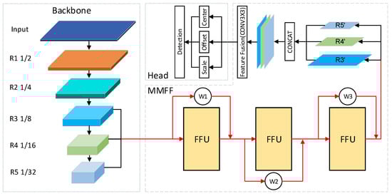
Figure 1.
Overall architecture of Adaptive Feature Fusion Detector (AFFDet). The red line represents the route with weights representing a series of weights that can be learned, and it is actually three routes with weights (corresponding to , and respectively).
3.2.1. Backbone Module
Res2Net-DLA-60 [21] is used as the backbone network, and light-weight ShuffleNet V2 [22] is also chosen as an extra backbone network. For convenience of description, we define the feature map obtained by stage n as . For Res2Net-DLA-60, we found that using , , and got the best performance through experiments, which are the feature maps with , , and times the size of the original image. And we use , , and in ShuffleNetV2, which are the feature maps with , , and times the size of the original image. In , the larger the number, the higher the feature level, and often the smaller the size. At the same time, because the scale reduction in feature maps is generally a multiple of 2, and the number of stages and the processing methods in different networks are different. In order to maintain consistency in the representations of different networks, we define that, with the increase of the network depth, the feature map whose size is scaled to the n-th power of 2 relative to the size of the input image is , thus , , and in Res2Net-DLA-60 correspond to , , and respectively. And , , and in ShuffleNetV2 correspond to , , and respectively. In , the smaller n, the larger the size, and the smaller the receptive field. At the same time, the utilized feature levels are lower, and the detection effect for small objects is better than that for large objects. Reversely, the larger n in , the smaller the size, but the larger the receptive field. At the same time, the utilized feature levels are higher, and the detection effect on large objects is better. However, because of its smaller size, the detection effect on small objects is not ideal, and some certain errors are prone to occur in object location.
3.2.2. Multi-Level Feature Fusion Module (MFFM)
In order to solve the disadvantages of different feature maps mentioned above with different sizes, and to improve the detection effect, we adopted some strategies to adaptively fuse multi-scale feature maps at multiple levels, that is MFFM, which is composed of its sub-module MFFU.
MFFU
The internal structure of MFFU is shown in Figure 2. First of all, we use step-by-step upsampling and fusion, and also step-by-step downsampling and fusion, but we only do it in , , and . Specifically, firstly, , , and are convoluted by 3 × 3 kernels. Then the convoluted , , and are bottom-up and top-down, respectively, and then connected horizontally. To solve the problem of original information loss after an MFFU, we add a shortcut structure. At the same time, for each process of feature fusion in the MFFU and the shortcut, how they achieves the best effect of feature fusion, we add the weight parameters that can be learned to every branch, which is denoted as in Figure 2, so that we can get the best fusion weights through training. In this way, more advantageous information can be contained in both the lower-level feature maps and the higher-level feature maps, and the feature map of each scale has a more consistent degree of feature fusion.
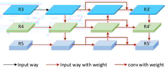
Figure 2.
Internal structure of MFFU. Through horizontal connection, vertical connection, shortcut and learnable weights, feature information is fused.
MFFM
In MFFM, if the number of MFFUs in MFFM is n, it is denoted as MFFM of . The connection form of MFFU in MFFM is shown in Figure 3.
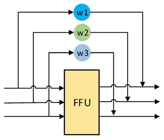
Figure 3.
Connection form of MFFU in MFFM, represents a weight that can be learned. The fusion ratio of each part depends on the shortcut and the learnable weight.
The input of the n-th MFFU is denoted as , and the processing of the n-th MFFU is denoted . At first, , , feature maps generated by the backbone network are taken as inputs, and it is specifically denoted as . For any n-th MFFU, its input is processed by the n-th MFFU, then multiplied by the learnable adaptive weights , and will be added with multiplied by the learnable adaptive weights . The result of that is used as the input of the (n + 1)-th MFFU. The formula is described as follows:
Within each MFFU, where , , .
In which represents the weight in the weighted training branch corresponding to feature map () in , and is obtained by the following process:
The advantage of such processing is that, as the number of MFFUs in MFFM increases, the lower-level features become less and less, and many of them are advantageous for detection. The weight of features in each stage can be adaptively determined by parameter W, which is equivalent to adding a special attention mechanism. It can make the training process smoother, and the effect is also better.
The feature maps with scales of , and after n MFFUs have fused features of different scales at multiple levels. These three feature maps are all deconvolved into scale, and then concatenated into one feature map. Then, the dimensions of the concatenated feature map will be compressed through a 3 × 3 convolution layer to further fuse features, consequently the final feature map is generated.
3.2.3. Detection Head
The output of the MFFM is the input of the detection head, and the multi-scale features in MFFM have been fully fused for detection. And then three prediction branches are used to predict on the final feature map . Specifically, the first branch uses a 1 × 1 convolution layer to process to generate the center heatmap. The second branch performs a 1 × 1 convolution layer to obtain the offset of the center point. The location and score of the center point of the object can be obtained through the center heatmap. However, because the scale of is down-sampled compared with the original image scale, the predicted location directly using the center heatmap will have deviation, which will result in inaccurate positioning. Thus, the offset branch is just to learn this deviation to offset it. In the third branch, a 1 × 1 convolution layer is performed to generate the scale map, and the length and width of scale values of each object corresponding to each center are obtained.
3.3. Loss Function
The total loss function consists of three parts, which correspond to the three prediction branches of the network.
Center Prediction Loss
First of all, for the center prediction branch, we directly transform it into a classification problem, and each pixel is assigned a classification score, so we use the cross-entropy loss commonly used in classification problems. Because the center point often predicted by this branch may not be the actual center point. For example, the predicted center point is the adjacent point of the actual center point, and the effect is still very good. However, it will be directly recognized as a recognition error, which is obviously inappropriate and difficult to train. Thus, we need to use a two-dimensional Gaussian mask besides locating the center point positive and determining other points as negative. Let the points around the center point have a certain weight according to Gaussian distribution. The closer to the center point, the higher the weight, which is advantageous for convergence, makes the training process smoother and predicts the center point easier. This Gaussian mask can be formulated as:
In which i and j represent the i-th row and the j-th column of the feature map respectively, thus i and j represent a single pixel when combined. k represents the k-th object in the image, and , , , respectively represent the abscissa, ordinate, width, and height of the center point of the k-th object. represents the Gaussian kernel used to control the range of Gaussian mask. If Gaussian masks overlap, the maximum value is taken as the value of the overlapping part. represents the Gaussian mask value of the point.
The loss function of the center branch is as shown above. In which, , , and s indicates the scaling factor of the original image compared with the current feature map.
Since pedestrian detection is often extremely imbalanced in samples and many negative samples are very similar to positive samples, we refer to the focal loss and give a smaller weight to a large number of samples that are easy to classify but give greater weight to samples that are difficult to classify. The formulas for and in the above formula are as follows:
represents the probability that the object center point exists at the point predicted by the model, with the value ranging from 0 to 1. While represents the ground truth of the point, with the value being 0 or 1. When is 1, it means that it is the actual object center point, while 0 means the negative point. Among them, and are two hyperparameters, and is used to reduce the weight of easily classified samples. Experiments show that the best performance is got when is set to 2, is used to adjust the penalty degree of Gaussian mask, and 4 for is the best.
Offset Prediction Loss
With the offset prediction branch, the model can learn the offset value between the actual center point and the scaled center point. We use SmoothL1 loss to penalize for ease of training and convergence. Its losses are as follows:
Among them, represents the ground-truth offset value after scaling at the point and represents the predicted offset value after scaling at the point. Therefore, , .
Scale Prediction Loss
For the scale prediction branch, similar to the center offset branch, we also used SmoothL1 loss, except that we took the actual size logarithm, which makes the training process easier to proceed. Its loss is as follows:
where, represents the scaled which represents ground truth of the object size at point, and represents the scaled which represents the object size predicted by the model. Thus and . and are used because logarithm loss makes the training process smoother and easier to train.
Final Detection Loss
The final detection loss is composed of the above three items which are center loss, offset loss and scale loss. The total loss formula is as follows:
In which, the hyperparameter is set to 0.1, is set to 1 and is set to 10.
3.4. Inference
The process of inference is shown in Figure 4.
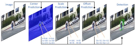
Figure 4.
Inference Process. When inferring, the three branches of the detection head is used to infer where there are the objects in the image, how many offsets are needed, and what are the sizes of the objects. In the figure, p represents the probability of being an object, and represent the coordinates of the center point of the object, H and W represent the height and width of the object, and represent the offset of the abscissa and ordinate of the object, and the bounding box can be obtained.
Particularly, in the center heatmap, if the confidence score is less than the threshold value , it will be set to 0; if it is greater than , it is reserved. Then NMS processing with the threshold value is performed to remove a plurality of predicted center points of the same object which may exist, and the remaining point is denoted as . The predicted value of the offset branch is ; the height and width values in the corresponding scale map of the point are and respectively. Thus, the coordinates of the bounding box can be obtained by the following formulas:
4. Experiments
4.1. Datasets
We used Caltech Pedestrian Detection Benchmark [23], which is one of the most widely recognized and challenging benchmarks for pedestrian detection. Caltech is composed of about 10 h of videos with a resolution of 640 × 480, which contains nearly 13 K people. These videos are recorded from the roads where vehicles are driving in the regular traffic environment in urban areas, which are basically consistent with the real environment. The training set enhanced by [24] is used, which takes one frame every three frames, totaling 42,782 frames, and the standard test set containing 4024 frames is used.
Because there are only about one-fifth of the images (positive samples) with pedestrians in the training set, the positive and negative samples are seriously out of balance. In order to alleviate this problem, we set the positive and negative samples of the training set to half the size of the training set by unequal sampling, 1024 samples respectively.
4.2. Evaluate Standard
The evaluation standard used by Caltech is log-average Miss Rate over False Positive Per Image (FPPI) ranging in , which is denoted as , and the lower curves or the smaller numbers indicate the better performance. In this paper, the default refers to the Reasonable setting which is the general setting with , and it will be specifically indicated if it is IoU = 0.75 setting.
FPS stands for frames per second, which is a unit for measuring the speed of a model, and the larger value indicate the faster speed. When testing, we set the mini-batch to 1.
The Params or the parameters represents the number of total parameters in the model, which measures the size and complexity of the model. The larger the value, the larger the model. In this paper, its unit is usually mega which is denoted as M.
4.3. Training
We implemented the proposed method on Pytorch [25], and the training and inference process are completed on one RTX 2080Ti GPU. We use the Mixed Precision [26] strategy to train in the whole process, aiming at accelerating the training speed by nearly 30% at the expense of little precision and developing the algorithm quicker. The selected backbone network are Res2Net-DLA-60 and ShuffleNetv2, which are pretrained on ImageNet [27], and are truncated on the basis of the original networks. Adam [28] is chosen as the optimizer. For Caltech, we used a mini-batch contains 8 images for Res2Net-DLA-60 and a mini-batch contains 32 images for ShuffleNetv2. The dynamic learning rate of warm-up cosine is used, the initial learning rate is , and the lowest learning rate is . The total training iterations is 204.8 K. It should be noted that due to the limitation of our conditions, we only used 2048 training samples instead of all 42,782 training samples for training. We take 0.41 as a fixed aspect ratio to strengthen training, and if we don’t do this, we can also complete the detection with a slight decrease in accuracy. We use the mean-teacher [29] strategy, which makes the previous training process teach the later training process, making the training process smoother. In the first epoch of the training process, , and in the subsequent epochs, . In which, represents the final model weights of the current epoch, and represents the final model weights of the last epoch. represents model weights after the current epoch training. is a hyperparameter that represents the ratio of occupies , and it is set to 0.001.
Only very simple and fundamental data augmentation techniques are adopted: random brightness, horizontal flip, random resize, and random padding.
4.4. Backbone Networks
Res2Net-DLA-60
The innovative Res2Net Module proposed in Res2Net replaces a group of 3 × 3 convolution layers in the network with a smaller group of 3 × 3 convolution layers and connects different filter groups in a hierarchical residual-like [30] style. With the Res2Net Module, more levels of receptive fields and the stronger ability of multi-scale representation are obtained.
Deep Layer Aggregation (DLA) [31] is an image classification network, which mainly introduces two structures: Iterative Deep Aggregation (IDA) and Hierarchical Deep Aggregation (HDA). IDA focuses on fusing different scales and resolutions, while HDA focuses on fusing all modules and channels. The combination of the two is manifested in the form that many hierarchical skip connections are used to fuse the features of different scales and stages.
The Res2Net-DLA-60 is a network obtained by replacing the common convolution structure in DLA with Res2Net Module. We removed the global pooling layer and full connection layer in Res2Net-DLA-60 and frozen the stage1, stage2 and stage3 for easier training. Then, using the outputs of stage4, stage5 and stage6, that are the scales of , and and the channels of 256, 512 and 1024, respectively.
The number of intermediate channels processed in MFFU in Res2Net-DLA-60 is 256
ShuffleNetV2
ShuffleNetV2 is a light-weight image classification network, which presents practical guidelines and novel architecture. It focuses on reducing computational complexity.
We removed the global pooling layer and full connection layer in ShuffleNetV2 and frozen the first convolution layer for easier training. Then, using the outputs of stage2, stage3, and stage4, which are the scales of , , and and the channels of 116, 232, and 464, respectively.
The number of intermediate channels processed in MFFU in ShuffleNetV2 is 116.
4.5. Ablation Study
Comparisons of Different Architectures of MFFM
In order to illustrate the proposed method, we have carried out many comparative experiments. These experiments are all done on the Caltech benchmark. These results were obtained from an average of five runs.
Table 1 shows the comparisons of the main experimental methods. Under the condition of no shortcut structure and only adding 3 MFFUs to Res2Net-DLA-60 directly, the performance has been obviously improved, from 4.75% to 4.31%, and the effect has also been improved to 4.16% when 6 MFFUs are added directly. This shows that our MFFU can directly improve the performance as a feature fusion unit when used only in series connection. If the shortcut structure without weights is directly added, the accuracy will be reduced whenever the levels are 3 or 6, compared with no shortcut structure. However, when the shortcut structure with weights is added, the effect has been greatly improved, which is far better than the no shortcut structure and the shortcut structure without weights. The results show that after adding MFFM of weighted shortcut structure with 3 MFFUs, compared with the case without MFFM, has been significantly improved from 4.75% to 3.65%, and the number of model parameters is reduced from 42 M to 40 M, although the speed is reduced from 36.7 to 32.3. When the number of MFFUs of MFFM is 6, the speed is further reduced to 28.0, but the is 3.71% without further improvement, probably because the features after 3 MFFUs are high enough for detection. The performance of 6 MFFUs and 3 MFFUs is basically the same under the setting, but the accuracy of 6 MFFUs is lower under setting.

Table 1.
Comparisons of Different Architectures of Multi-Level Feature Fusion Module (MFFM). In which, R2-DLA represents Res2Net-DLA-60 and SNv2 represents ShuffleNetV2. And shortcut/n means no shortcut structure in the MFFM, and weights/n indicates that there are shortcut structures but without learnable weights in MFFM and weights/w indicates that there are shortcut structures with learnable weights. The number below MFFM (level=) represents how many Multi-Scale Feature Fusion Units (MFFUs) are added in the corresponding connection form of MFFM.
After adding MFFM with level = 3, compared with the ShuffleNetV2 without MFFM, improved significantly from 14.35% to 11.97%, the model parameters decreased from 5.2 M to 4.8 M, but the speed decreased from 58.7 to 45.0.
No matter whether the backbone network is Res2Net-DLA-60 or ShuffleNetV2, its performance has obviously improved after adding MFFM of . And both the parameters of the two networks are reduced after adding MFFM of , but the speeds are decreased.
Comparisons of Different External Structures of MFFUs
In terms of the connection modes of MFFUs in MFFM, we have tried many different structures. Their structures are shown in Figure 5, and their experimental results are shown in Table 2. For (a) structure in Figure 5, the feature maps output from the previous MFFUs and the original feature map output from the backbone are added with weights and then input to the current MFFU. In this way, the deep structure can retain some original and lower-level features, but its experimental performance is not good, and its is 4.12% when level = 3. For (b) structure in Figure 5, the output of all MFFUs before the last MFFU and the original feature map output by backbone are added in the form of weights and then output to the last MFFU for processing, but it may be that the last MFFU cannot process and fuse so much information well. This method is not effective, and its is 4.35% when level = 3. For (c) structure in Figure 5, starting from the original feature map output by backbone, the weighted addition of the output of the current MFFU and the shortcut of the input of the current MFFU has the best effect, and its MR is 3.65% at level = 3, far better than that of (a) and (b). Among the three structures, (a) is the fastest and (c) is the slowest, but there is just slight difference in the overall speed. (a), (b) and (c) are 35.9, 35.1 and 32.3 respectively when level = 3. Experiments show that (c) structure of our MFFM has the best comprehensive performance and speed, and has great advantages.
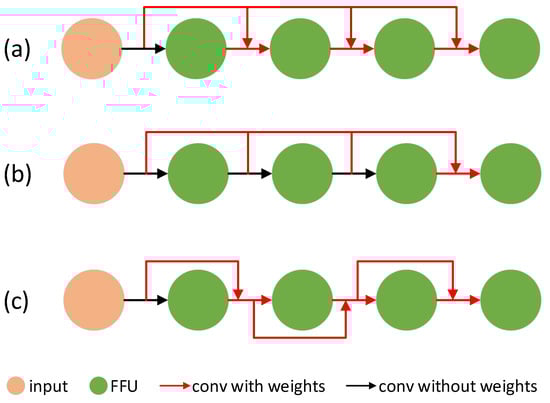
Figure 5.
Different external structures of MFFUs in MFFM. (a–c) are three different structures.
Table 2.
Comparisons of different external structures of MFFUs on Caltech. In which, The number under level= represents the number of MFFUs in MFFM.
4.6. Comparisons with Other Methods
We use Caltech as a benchmark. Figure 6 shows the comparisons with other methods under the setting, Figure 7 shows the comparisons with other methods under setting, and more methods are compared in Table 3. AFFDet, our proposed method, achieves 3.7% under the setting, which is 0.8% better than the closest CSP’s 4.5%. Compared with the stricter setting, we are even more ahead, and have achieved 21.0% , which is 4.8% better than the closest CSP’s 25.8%. And in terms of speed, our AFFDet achieved 32.3, which is faster than the officially implemented CSP’s 23.6. For the case of heavy occlusion, we also achieved 43.2%, which has a better effect of more than 4% compared with 47.9% of RepLoss detector specially designed for occlusion problem. This shows that our adaptive multi-level and multi-scale feature fusion method is very effective in pedestrian detection, and our performance is ahead of other methods.
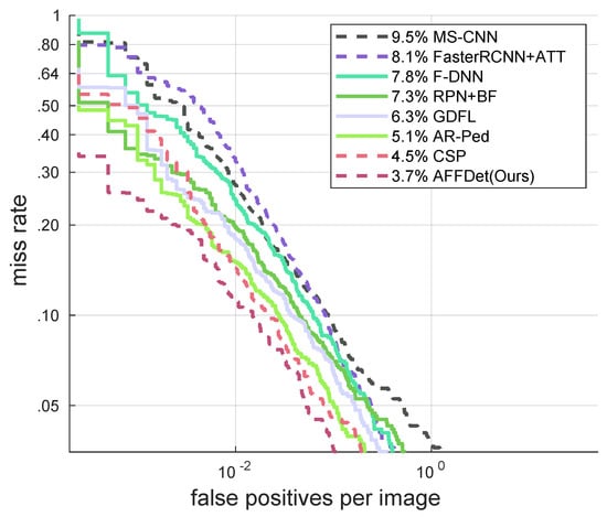
Figure 6.
Comparisons with other methods under IoU = 0.5 setting on Caltech.
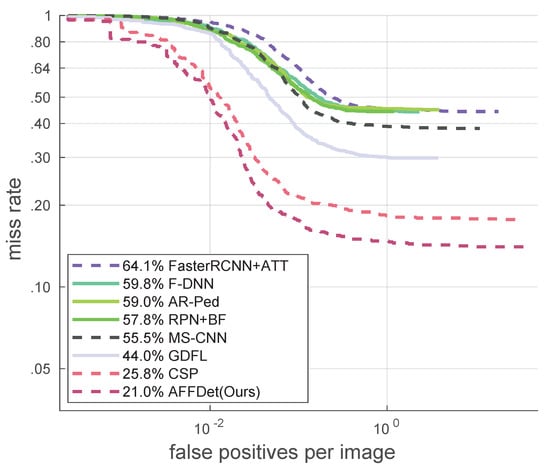
Figure 7.
Comparisons with other methods under IoU = 0.75 setting on Caltech.
Table 3.
Comparisons with other methods on Caltech.
5. Discussion and Conclusions
In order to solve the problems of inadequate feature utilization and inadequate feature fusion in previous pedestrian detectors, we propose AFFDet. As its name suggests, the original adaptive feature fusion methods are the main contributions of this work. Specifically, AFFDet is a detector that uses our original adaptive multi-level and multi-scale feature fusion methods to get the best features for detection, and our innovative MFFU and MFFM play a vital role in it. Among them, MFFU reflects adaptive multi-scale feature fusions, and MFFM reflects adaptive multi-level feature fusions. In the field of pedestrian detection, the proposed AFFDet has achieved leading detection results in the Caltech benchmark. It is the state-of-the-art one-stage pedestrian detector at present with competitive speed as an anchor-free one-stage approach. According to our experiments, MFFU can be used independently as a feature fusion module, which can improve the model performance. Compared with many feature fusion modules like MFFU which are simply connected together, MFFM structure can further improve the performance. Great performance has been achieved by our proposed detector when only very simple data augmentation techniques are adopted and a small part of samples are used for training due to the limitation of our conditions. Theoretically, training with some powerful data augmentation techniques used in many detection methods and more training samples can further improve the performance. When the number of MFFU in MFFM is 3, it already achieved excellent results, and it does not increase the parameters of the model but only slightly reduces the speed.
Since Caltech is a dataset recorded by car cameras in the regular traffic scenes in different cities, which is basically consistent with the scenes in real life, the excellent performance of the proposed method on Caltech can basically continue to real life. However, in the real scene, especially in some scenes that need high-resolution detection, the computation of this method is too large, and it is difficult to achieve the speed of real-time detection. The follow-up work will mainly focus on reducing the amount of computation and improving the speed of the model while keeping the current performance basically unchanged or slightly reduced. It will be divided into a high-performance network and a high-efficiency network for high-precision detection scenarios and high-speed detection scenarios to further improve the practicality. We will also verify our method in more fields such as vehicle detection and more datasets.
Author Contributions
Conceptualization, Y.X.; methodology, Y.X. and Q.Y.; software, Y.X.; validation, Y.X.; writing—original draft preparation, Y.X.; writing—review and editing, Y.X. and Q.Y.; supervision, Q.Y.; project administration, Q.Y. All authors have read and agreed to the published version of the manuscript.
Funding
This research received no external funding.
Data Availability Statement
The data presented in this study are openly available in Computational Vision at Caltech at http://www.vision.caltech.edu/Image_Datasets/CaltechPedestrians/, reference number [23].
Conflicts of Interest
The authors declare no conflict of interest.
References
- Girshick, R.; Donahue, J.; Darrell, T.; Malik, J. Rich feature hierarchies for accurate object detection and semantic segmentation. In Proceedings of the IEEE conference on computer vision and pattern recognition, Columbus, OH, USA, 23–28 June 2014; pp. 580–587. [Google Scholar]
- Ren, S.; He, K.; Girshick, R.; Sun, J. Faster r-cnn: Towards real-time object detection with region proposal networks. IEEE Trans. Pattern Anal. Mach. Intell. 2016, 39, 1137–1149. [Google Scholar] [CrossRef] [PubMed]
- Liu, W.; Anguelov, D.; Erhan, D.; Szegedy, C.; Reed, S.; Fu, C.Y.; Berg, A.C. Ssd: Single shot multibox detector. In European Conference on Computer Vision; Springer: Berlin/Heidelberg, Germany, 2016; pp. 21–37. [Google Scholar]
- Lin, T.Y.; Dollár, P.; Girshick, R.; He, K.; Hariharan, B.; Belongie, S. Feature pyramid networks for object detection. In Proceedings of the IEEE Conference on Computer Vision and Pattern Recognition, Honolulu, HI, USA, 21–26 July 2017; pp. 2117–2125. [Google Scholar]
- Girshick, R. Fast r-cnn. In Proceedings of the IEEE International Conference on Computer Vision, Santiago, Chile, 7–13 December 2015; pp. 1440–1448. [Google Scholar]
- He, K.; Gkioxari, G.; Dollár, P.; Girshick, R. Mask r-cnn. In Proceedings of the IEEE International Conference on Computer Vision, Santiago, Chile, 7–13 December 2017; pp. 2961–2969. [Google Scholar]
- Cai, Z.; Vasconcelos, N. Cascade r-cnn: Delving into high quality object detection. In Proceedings of the IEEE Conference on Computer Vision and Pattern Recognition, Salt Lake City, UT, USA, 18–23 June 2018; pp. 6154–6162. [Google Scholar]
- Dai, J.; Li, Y.; He, K.; Sun, J. R-fcn: Object detection via region-based fully convolutional networks. arXiv 2016, arXiv:1605.06409. [Google Scholar]
- Zhang, L.; Lin, L.; Liang, X.; He, K. Is faster R-CNN doing well for pedestrian detection? In European Conference on Computer Vision; Springer: Berlin/Heidelberg, Germany, 2016; pp. 443–457. [Google Scholar]
- Cai, Z.; Fan, Q.; Feris, R.S.; Vasconcelos, N. A unified multi-scale deep convolutional neural network for fast object detection. In European Conference on Computer Vision; Springer: Berlin/Heidelberg, Germany, 2016; pp. 354–370. [Google Scholar]
- Wang, X.; Xiao, T.; Jiang, Y.; Shao, S.; Sun, J.; Shen, C. Repulsion loss: Detecting pedestrians in a crowd. In Proceedings of the IEEE Conference on Computer Vision and Pattern Recognition, Salt Lake City, UT, USA, 18–23 June 2018; pp. 7774–7783. [Google Scholar]
- Lin, T.Y.; Goyal, P.; Girshick, R.; He, K.; Dollár, P. Focal loss for dense object detection. In Proceedings of the IEEE International Conference on Computer Vision, Santiago, Chile, 7–13 December 2017; pp. 2980–2988. [Google Scholar]
- Liu, W.; Liao, S.; Hu, W.; Liang, X.; Chen, X. Learning efficient single-stage pedestrian detectors by asymptotic localization fitting. In Proceedings of the European Conference on Computer Vision (ECCV), Munich, Germany, 8–14 September 2018; pp. 618–634. [Google Scholar]
- Huang, L.; Yang, Y.; Deng, Y.; Yu, Y. Densebox: Unifying landmark localization with end to end object detection. arXiv 2015, arXiv:1509.04874. [Google Scholar]
- Redmon, J.; Divvala, S.; Girshick, R.; Farhadi, A. You only look once: Unified, real-time object detection. In Proceedings of the IEEE Conference on Computer Vision and Pattern Recognition, Las Vegas, NV, USA, 27–30 June 2016; pp. 779–788. [Google Scholar]
- Law, H.; Deng, J. Cornernet: Detecting objects as paired keypoints. In Proceedings of the European Conference on Computer Vision (ECCV), Munich, Germany, 8–14 September 2018; pp. 734–750. [Google Scholar]
- Lu, X.; Li, B.; Yue, Y.; Li, Q.; Yan, J. Grid r-cnn. In Proceedings of the IEEE Conference on Computer Vision and Pattern Recognition, Long Beach, CA, USA, 15–21 June 2019; pp. 7363–7372. [Google Scholar]
- Tian, Z.; Shen, C.; Chen, H.; He, T. Fcos: Fully convolutional one-stage object detection. In Proceedings of the IEEE International Conference on Computer Vision, Seoul, Korea, 27 October–2 November 2019; pp. 9627–9636. [Google Scholar]
- Duan, K.; Bai, S.; Xie, L.; Qi, H.; Huang, Q.; Tian, Q. Centernet: Keypoint triplets for object detection. In Proceedings of the IEEE International Conference on Computer Vision, Seoul, Korea, 27 October–2 November 2019; pp. 6569–6578. [Google Scholar]
- Liu, W.; Liao, S.; Ren, W.; Hu, W.; Yu, Y. High-level semantic feature detection: A new perspective for pedestrian detection. In Proceedings of the IEEE Conference on Computer Vision and Pattern Recognition, Long Beach, CA, USA, 15–21 June 2019; pp. 5187–5196. [Google Scholar]
- Gao, S.; Cheng, M.M.; Zhao, K.; Zhang, X.Y.; Yang, M.H.; Torr, P.H. Res2Net: A New Multi-Scale Backbone Architecture. IEEE Trans. Pattern Anal. Mach. Intell. 2021, 43, 652–662. [Google Scholar] [CrossRef] [PubMed]
- Ma, N.; Zhang, X.; Zheng, H.T.; Sun, J. Shufflenet v2: Practical guidelines for efficient cnn architecture design. In Proceedings of the European Conference on Computer Vision (ECCV), Munich, Germany, 8–14 September 2018; pp. 116–131. [Google Scholar]
- Dollár, P.; Wojek, C.; Schiele, B.; Perona, P. Pedestrian detection: A benchmark. In 2009 IEEE Conference on Computer Vision and Pattern Recognition; IEEE: Piscataway, NJ, USA, 2009; pp. 304–311. [Google Scholar]
- Zhang, S.; Benenson, R.; Omran, M.; Hosang, J.; Schiele, B. How far are we from solving pedestrian detection? In Proceedings of the IEEE Conference on Computer Vision and Pattern Recognition, Las Vegas, NV, USA, 27–30 June 2016; pp. 1259–1267. [Google Scholar]
- Paszke, A.; Gross, S.; Massa, F.; Lerer, A.; Bradbury, J.; Chanan, G.; Killeen, T.; Lin, Z.; Gimelshein, N.; Antiga, L.; et al. PyTorch: An Imperative Style, High-Performance Deep Learning Library. In Proceedings of the Advances in Neural Information Processing Systems, Vancouver, BC, Canada, 8–14 December 2019; pp. 8026–8037. [Google Scholar]
- Micikevicius, P.; Narang, S.; Alben, J.; Diamos, G.; Elsen, E.; Garcia, D.; Ginsburg, B.; Houston, M.; Kuchaiev, O.; Venkatesh, G.; et al. Mixed precision training. arXiv 2017, arXiv:1710.03740. [Google Scholar]
- Deng, J.; Dong, W.; Socher, R.; Li, L.J.; Li, K.; Fei-Fei, L. Imagenet: A large-scale hierarchical image database. In 2009 IEEE Conference on Computer Vision and Pattern Recognition; IEEE: Piscataway, NJ, USA, 2009; pp. 248–255. [Google Scholar]
- Kingma, D.P.; Ba, J. Adam: A method for stochastic optimization. arXiv 2014, arXiv:1412.6980. [Google Scholar]
- Tarvainen, A.; Valpola, H. Mean teachers are better role models: Weight-averaged consistency targets improve semi-supervised deep learning results. In Proceedings of the Advances in Neural Information Processing Systems, Long Beach, CA, USA, 4–9 December 2017; pp. 1195–1204. [Google Scholar]
- He, K.; Zhang, X.; Ren, S.; Sun, J. Deep residual learning for image recognition. In Proceedings of the IEEE Conference on Computer Vision and Pattern Recognition, Las Vegas, NV, USA, 26 June–1 July 2016; pp. 770–778. [Google Scholar]
- Feng, Z.; Jin, L.; Tao, D.; Huang, S. DLANet: A manifold-learning-based discriminative feature learning network for scene classification. Neurocomputing 2015, 157, 11–21. [Google Scholar] [CrossRef]
- Zhang, S.; Yang, J.; Schiele, B. Occluded pedestrian detection through guided attention in cnns. In Proceedings of the IEEE Conference on Computer Vision and Pattern Recognition, Salt Lake City, UT, USA, 18–23 June 2018; pp. 6995–7003. [Google Scholar]
- Mao, J.; Xiao, T.; Jiang, Y.; Cao, Z. What can help pedestrian detection? In Proceedings of the IEEE Conference on Computer Vision and Pattern Recognition, Honolulu, HI, USA, 21–26 July 2017; pp. 3127–3136. [Google Scholar]
- Perez, D.; Hasan, M.; Shen, Y.; Yang, H. Ar-ped: A framework of augmented reality enabled pedestrian-in-the-loop simulation. Simul. Model. Pract. Theory 2019, 94, 237–249. [Google Scholar] [CrossRef]


Publisher’s Note: MDPI stays neutral with regard to jurisdictional claims in published maps and institutional affiliations. |
© 2021 by the authors. Licensee MDPI, Basel, Switzerland. This article is an open access article distributed under the terms and conditions of the Creative Commons Attribution (CC BY) license (http://creativecommons.org/licenses/by/4.0/).