Online Service Function Chain Deployment for Live-Streaming in Virtualized Content Delivery Networks: A Deep Reinforcement Learning Approach

Abstract

Video delivery is exploiting 5G networks to enable higher server consolidation and deployment flexibility. Performance optimization is also a key target in such network systems. We present a multi-objective optimization framework for service function chain deployment in the particular context of Live-Streaming in virtualized content delivery networks using deep reinforcement learning. We use an Enhanced Exploration, Dense-reward mechanism over a Dueling Double Deep Q Network (E2-D4QN). Our model assumes to use network function virtualization at the container level. We carefully model processing times as a function of current resource utilization in data ingestion and streaming processes. We assess the performance of our algorithm under bounded network resource conditions to build a safe exploration strategy that enables the market entry of new bounded-budget vCDN players. Trace-driven simulations with real-world data reveal that our approach is the only one to adapt to the complexity of the particular context of Live-Video delivery concerning the state-of-art algorithms designed for general-case service function chain deployment. In particular, our simulation test revealed a substantial QoS/QoE performance improvement in terms of session acceptance ratio against the compared algorithms while keeping operational costs within proper bounds.

1. Introduction

Video traffic occupies more than three-quarters of total internet traffic nowadays, and the trend is to grow [1]. Such growth is mainly characterized by Over-The-Top (OTT) video delivery. Content providers need OTT Content Delivery systems to be efficient, scalable, and adaptive [2]. For this reason, cost and Quality of Service (QoS) optimization for video content delivery systems is an active research area. A lot of the research effort in this context is being placed on the optimization [3], and modeling [4] of Content Delivery systems’ performance.

Content Delivery Networks (CDN) are distributed systems that optimize the end-to-end delay of content requests over a network. CDN systems are based on the redirection of requests and content reflection. Well-designed CDN systems warrant good Quality of service (QoS) and Quality of Experience (QoE) for widely distributed users. CDN uses replica servers as proxies for the content providers’ origin servers. Traditional CDN systems are deployed on dedicated hardware and incur, thereby in high capital and operational expenditures. On the other hand, virtualized Content Delivery Networks (vCDN) use Network Function Virtualization (NFV) [5], and Software-defined Networking (SDN) [6] to deploy their software components on virtualized network infrastructures like virtual machines or containers. NFV and SDN are key enablers for 5G networks [7]. Over the last two years, numerous internet services providers (ISP), mobile virtual network operators (MVNO), and other network market players are exploiting 5G networks to augment the spectrum of network services they offer [8]. In this context, virtualized CDN systems are taking the profit of 5G networks to enable higher server consolidation, and flexibility during deployment [9,10]. VCDNs reduce both capital and operational expenditures concerning CDNs deployed to dedicated-hardware [11]. Further, vCDNs are edge-computing compliant [12] and make possible to act win-win strategies between ISP and CDN providers [13].

1.1. Problem Definition

Virtualized Network systems are usually deployed as a composite chain of Virtual Network Functions (VNF), often called a service function chain (SFC). Every incoming request to a virtualized network system will be mapped to a corresponding deployed SFC. The problem of deploying a SFC inside a VNF infrastructure is called VNF Placement or SFC Deployment [14]. Many service requests can share the same SFC deployment scheme, or the SFC deployments can vary. Given two service requests that share the same requested chain of VNFs, the SFC deployment will vary when at least one pair of same-type VNFs are deployed on different physical locations for each request.

This work focuses on the particular case of Live-Video delivery, also referred to as live-streaming. In such a context, each service request is associated with a Live-Video streaming session. CDNs have proved essential to meet scalability, reliability, and security in Live-Video delivery scenarios. One important Quality of Experience (QoE) measure in live-video streaming is the session startup delay, which is the time the end-user waits since the content is requested and the video is displayed. One important factor that influences the startup delay is the round-trip-time (RTT) of the session request, which is the time between the content request is sent, and the response is received. In live-Streaming, the data requested by each session is determined only by the particular content provider or channel requested. Notably, cache HIT and cache MISS events may result in very different request RTTs. Consequently, a realistic Live-Streaming vCDN model should keep track of the caching memory status of every cache-VNF module for fine-grain RTT simulation.

Different SFC deployments may result in different round-trip times (RTT) for live-video sessions. The QoS/QoE goodness of a particular SFC deployment policy is generally measured by the mean acceptance ratio (AR) of client requests, where the acceptance ratio is defined as the percentage of requests whose RTT is below a maximum threshold [14,15,16]. Notice that RTT is different from the total delay, which is the total propagation time of the data stream from the origin server and the end-user.

Another important factor that influences RTT computation is the request processing time. Such a processing time will notably depend on the current VNF utilization. To model VNF utilization in a video-delivery context, major video streaming companies [17] recommend to consider not only the content-delivery tasks, but also the resource consumption associated with content-ingestion processes. In other words, any VNF must ingest a particular data stream before being able to deliver it through its own client connections, and such ingestion will incur non-negligible resource usage. Further, a realistic vCDN delay model must incorporate VNF instantiation times, as they may notably augment the starting delay of any video-streaming session. Finally, both instantiation time and resource consumption may differ significantly depending on the specific characteristics of each VNF [3].

In this paper, we model a vCDN following the NFV Management and orchestration (NFV-MANO) framework published by the ETSI standard group specification [9,18,19,20]. We propose elastic container-based virtualization of a CDN inspired by [5,19]. One of the management software components of a vCDN in the ETSI standard is the Virtual Network Orchestrator (VNO), which is generally responsible for the dynamic scaling of the containers’ resource provision [19]. The resource scaling is triggered when needed, for example, when traffic bursts occur. Such a resource scaling may influence the resource provision costs, also called hosting costs, especially if we consider a cloud-hosted vCDN context [20]. Also, data-transportation (DT) routes in the substrate network of a vCDN may be affected by different SFC deployment decisions. Consequently, DT costs may also vary [9], especially if we consider a multi-cloud environment as we do in this work. Thus, DT costs may also be an important part of the operational costs of a vCDN.

Finally, Online SFC Deployment implies taking fine-grained control decisions over the deployment scheme of SFCs when the system is running. For example, one could associate one SFC deployment for each incoming request to the system or keep the same SFC deployment for different requests but be able to change it whenever requested. In all cases, Online SFC Deployment implies that SFC policy adaptions can be done each time a new SFC request comes into the system. Offline deployment instead takes one-time decisions over aggregations of input traffic to the system [21]. Offline optimization’s effectiveness relies on the estimation accuracy of future environment characteristics [22]. Such estimation may not be trivial, especially in contexts where incoming traffic patterns may be unpredictable or when request characteristics might be heterogeneous, which is the case of Live-Streaming [9,14,23,24]. Consequently, in this work, we consider the Online optimization of a Live-Streaming vCDN SFC deployment, and we seek such optimization in terms of both QoS/QoE and operational costs, where the latter are composed of hosting costs and data-transportation costs.

1.2. Related Works

SFC Deployment is an NP-hard problem [25]. Several exact optimization models, and sub-optimal heuristics, have been proposed in recent years. Ibn-Khedher et al. [26] defined a protocol for optimal VNF placement based on SDN traffic rules and an exact optimization algorithm. This work solves the optimal VNF placement, migration, and routing problem, modeling various system and network metrics as costs and user satisfaction. HPAC [27] is a heuristic proposed by the same authors to scale the solutions of [26] for bigger topologies based on the Gomory-Hu tree transformation of the network. Their call for future work includes the need for the dynamic triggering of adaptation like monitoring user demands, network loads, and other system parameters. Yala et al. [28] present a resource allocation and VNF placement optimization model for vCDN and a two-phase offline heuristic for solving it in polynomial time. This work models server availability through an empirical probabilistic model and optimizes this score alongside the VNF deployment costs. Their algorithm produces near-optimal solutions in minutes for a Network Function Virtualization Infrastructure (NFVI) deployed on a substrate network made of even 600 physical machines. They base the dimensioning criteria on extensive video streaming VNF QoE-aware benchmarking.

Authors in [20] keep track of resource utilization in the context of an optimization model for multi-cloud placement of VNF chains. Utilization statistics per node and network statistics per link are taken into account inside a simulation/optimization framework for VNF placement in vCDN in [29]. This offline algorithm can handle large-scale graph topologies being designed to run on a parallel-supercomputer environment. This work analyzes the effect of routing strategies on the results of the placement algorithm and performs better with a greedy max-bandwidth routing approach. The caching state of each cache-VNF is modeled with a probabilistic function in this work. Offline Optimization of Value Added Service (VAS) Chains in vCDN is proposed in [30], where authors model an Integer Linear Programming (ILP) problem to optimize QoS and Provider Costs. This work models license costs for each VNF added in a new physical location. An online alternative is presented in [31], where authors model the cost of VNF instantiations when optimizing online VNF placement for vCDN. This model lacks to penalize the Roud Trip Time (RTT) of requests with the instantiation time of such VNFs. More scalable solutions for this problem are leveraged with heuristic-based approaches like the one in [32]. On the other hand, regularization-based techniques are used to present an online VNF placement algorithm for geo-distributed VNF chain requests in [32]. This work optimizes different costs and the end-to-end delay providing near-optimal solutions in polynomial time.

Robust Optimization (RO) has also been applied to solve various network-related optimization problems. RO and stochastic programming techniques have been used to model optimization under scenarios characterized by data uncertainty. Uncertainty concerning network traffic fluctuations or resource request amount can be modeled if one seeks to minimize network power consumption [33] or the costs related to cloud resource provisioning [34], for example. In [35], Marotta et. al. present a VNF placement and SFC routing optimization model that minimizes power consumption taking into account that resource requirements are uncertain and fluctuate in virtual Evolved Packet Core scenarios. Such an algorithm is enhanced in a successive work [36] where authors improve the scalability of their solution by dividing the task into sub-problems and adopting various heuristics. Such an improvement permits solving high-scale VNF placement in less than a second, making such an algorithm suitable for online optimization. Remarkably, the congestion-induced delay has been modeled in this work. Ito et. al. [37] instead provide various models of the VNF placement problem where the objective is to warrant probabilistic failure recovery with minimum backup required capacity. Authors in [37] model uncertainty in both failure events and virtual machine capacity.

Deep Reinforcement Learning (DRL) based approaches have been modeled to solve the SFC deployment also. DRL algorithms have recently evolved to solve problems on high-dimensional action spaces through the usage of state-space discretization [38], Policy Learning [39,40], and sophisticated Value learning algorithms [41]. Network-related problems like routing [42], and VNF forwarding graph embedding [43,44,45] have been solved with DRL techniques. Authors in [46] use the Deep Q-learning framework to implement a VNF placement algorithm which is aware of the server reliability. A policy learning algorithm is used for optimizing operational costs and network throughput on SFC Deployment optimization in [14]. A fault-tolerant version of SFC Deployment is presented in [47], where authors use a Double Deep Q-network (DDQN) and propose different resource reservation schemes to balance the waste of resources and ensure service reliability. Authors in [48] assume to have accurate incoming traffic predictions in input and use a DDQN based algorithm for choosing small-scale network sub-regions to optimize every 15 min. Such a work uses a threshold-based policy to optimize the number of fixed-dimensioned VNF instances. A Proximal Policy Optimization DRL scheme is used in [49] to jointly minimize packet loss and server energy consumption on a cellular network SFC deployment environment. The advantage of DRL approaches with respect to traditional optimization models is the constant time complexity reached after training. A well-designed DRL framework has the potential to achieve complex feature learning and near-optimal solutions even to unprecedented context situations [23].

1.3. Main Contribution

To the best of the authors’ knowledge, this work is the first VNF-SCF deployment optimization model for the particular case of Live-Streaming vCDN. We propose a vCDN model where we take into account, at the same time:

• VNF-instantiation times,
• Content-delivery and content-ingestion resource usage,
• Utilization-dependant processing times,
• Fine-grained cache-status tracking,
• Operational costs composed of data-transportation costs and hosting costs,
• Multi-cloud deployment characteristics,
• No a-priory knowledge of session duration.

We seek to jointly optimize QoS and operational costs with an Online DRL-based approach. To achieve this objective, we propose a dense-reward model and an enhanced-exploration mechanism for over a dueling-DDQN agent, which combination leads to the convergence to sub-optimal SFC deployment policies.

Further, in this work, we model bounded network resource availability to simulate network overload scenarios. Our aim is to create and validate a safe-exploration framework that facilitates the assessment of market-entry conditions for new cloud-hosted Live-Streaming vCDN operators.

Our experiments show that our proposed algorithm is the only one to adapt to the model conditions, maintaining an acceptance ratio above the state-of-art techniques for SFC deployment optimization while keeping a satisfactory balance between network throughput and operational costs. This paper can be seen as an upgrade proposal for the framework presented in [14]. The optimization objective of SFC deployment that we pursue is the same: maximizing the QoS and minimizing the operational costs. We enhance the algorithm used in [14] to find a suitable DRL technique for the particular case of Live-Streaming in v-CDN scenarios.

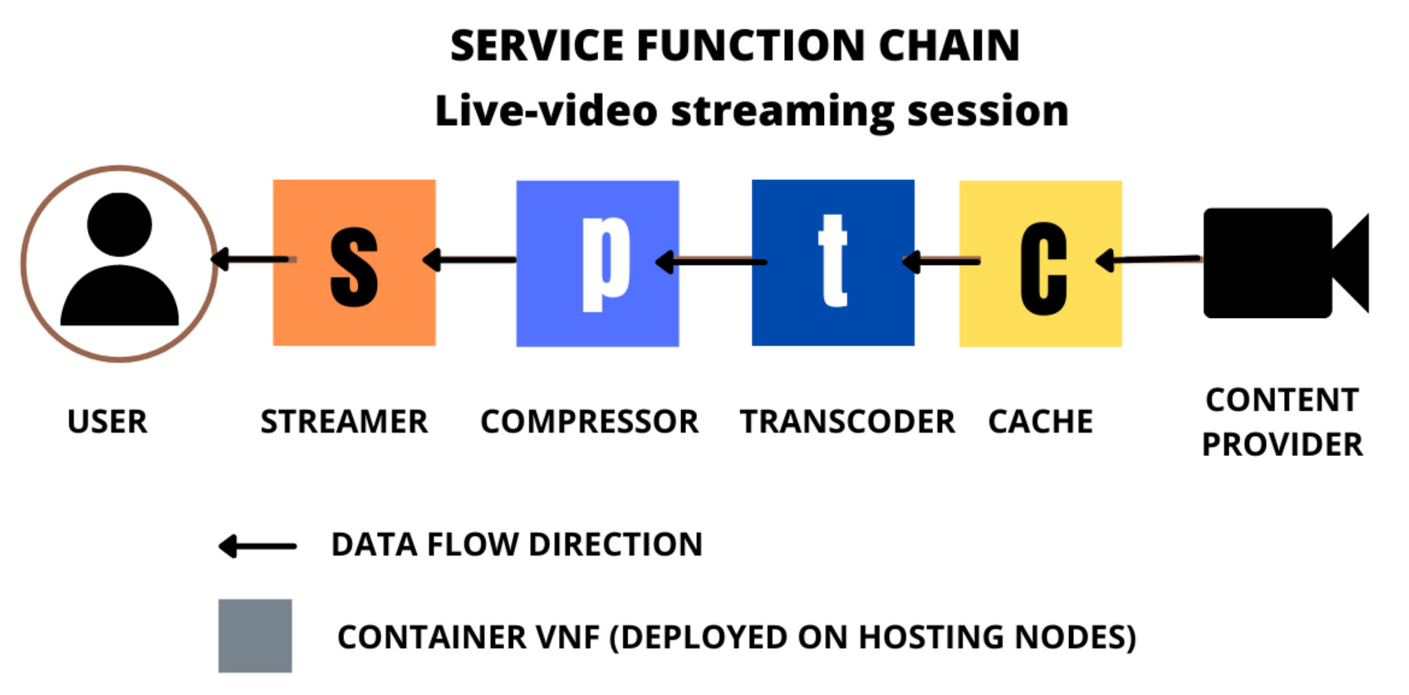
2. Materials and Methods

2.1. Problem Modelisation

We now rigorously model our SFC Deployment optimization problem. First of all, the system elements that are part of the problem are identified. We then formulate a high-level optimization statement briefly. Successively, our optimization problem’s decision variables, penalty terms, and feasibility constraints are described. Finally, we formally define the optimization objective.

2.1.1. Network Elements and Parameters

We model three-node categories in the network infrastructure of a vCDN. The content provider (CP) nodes, denoted as $N_{CP}$, produce live-video streams that are routed through the SFC to reach the end-users. The VNF hosting nodes, $N_H$, are the cloud-hosted virtual machines that instantiate container VNFs and interconnect through each other to form the SFCs. Lastly, we consider nodes representing geographic clusters of clients, $N_{UC}$. Geographic client clusters are created in such a way that every client in the same geographic cluster is considered to have the same data-propagation delays with respect to the hosting nodes in $N_H$. Client cluster nodes will be referred to as client nodes from now on. Notice that different hosting nodes may be deployed on different cloud providers. We denote the set of all nodes of the vCDN substrate network as:

$$N=N_{CP}\cup N_H\cup N_{UC}$$

We assume that each live-streaming session request r is always mapped to a VNF chain containing a Streamer, a Compressor, a Transcoder, and a Cache module [19,50]. In a live-streaming vCDN context, the caching module acts as a proxy that ingests video chunks from a Content Provider, stores them on memory, and sends them to the clients towards the rest of the SFC modules. Caching modules accelerate session startup time and prevent origin server overloads, keep an acceptable total delay, improving session startup times which is a measure of QoE in the context of live-streaming. Compressors, instead, may help to decrease video quality when requested. On the other hand, transcoding functionalities are necessary whenever the requested video codec is different from the original one. Finally, the streamer acts as a multiplexer for the end-users [19]. The order in which the VNF chain is composed is explained by Figure 1.

We will denote the set of VNF types considered in our model as K:

$$K=\{streamer,compressor,transcoder,cache\}$$

Any k-type VNF instantiated at a hosting node i will be denoted as $f_i^k,\forall k\in K,\forall i\in N_H$. We assume that every hosting node is able to instantiate a maximum of one k-type VNF. Note that, at any time, there might be multiple SFCs whose k-type module is assigned to a single hosting node i.

We define fixed-length time windows denoted as $t,\forall t\in \mathbb{N}$ which we call simulation time-steps following [14]. At each t, the VNO releases resources for timed-out sessions and processes the incoming session requests denoted as $R_t=\{r_1,r_2,...,r_{|R_t|}\}$. It should be stressed that every r will request for a SFC composed of all the VNF types in K. We will denote the k-type VNF requested by r as ${\widehat{f}}_r^k,\forall k\in K,r\in R_t$. Key notations for our vCDN SFC Deployment Problem are listed in

Table 1. Key notations for our vCDN SFC Deployment Problem.

Notation	Meaning
$N_{CP}$	The set of content-provider nodes
$N_H$	The set of VNF hosting nodes
$N_{UC}$	The set of user clusters
K	The set of VNF types (cache, compressor, transcoder, and streamer)
t	A fixed time-step in our simulation
$R_t$	The set of incoming SFC requests during time-step t
T	The max tolerable RTT for SFC any Live-Streaming request
$b_r$	The maximum scaled bitrate of r
$p_r$	The mean scaled session payload of r
${\widehat{f}}_r^k$	The k-type VNF requested by r
$l_r$	The channel or content provider requested by r
$s_r$	The session workload of r
${\gamma }_{res,i}$	The unit cost of $res$ resource in hosting node i
$d_{i,j}$	The data propagation delay between nodes i and j
$f_i^k$	The k-type VNF container instance in node i
$a_n^{t,k}$	1 if $f_n^k$ is instantiated at the beginning of t
$x_{r,i}^k$	1 if ${\widehat{f}}_r^k$ is assigned to node i, 0 otherwise
$z_{i,j,k}^r$	1 if the link between i and j is used to reach ${\widehat{f}}_r^k$, 0 otherwise
$y_{l,i,k}$	1 if $f_i^k$ is currently ingesting channel l, 0 otherwise
$c_{res,k,i}^t$	The $res$ resource provision in $f_i^k$ during t
${\sigma }_{k,r,res}$	The client $res$ resource demand of r in any k-type VNF instance
$v_{k,res}$	The $res$ resource demand for content ingestion in any k-type VNF instance
$u_{res,k,i}$	The current $res$ resource usage of $f_i^k$
${\mu }_{res,k,i}$	The current $res$ resource utilization of $f_i^k$
${\rho }_{res,i,k}^r$	The processing time contribution of $res$ resource in $f_i^k$ for ${\widehat{f}}_r^k$
${\varphi }_p$	The normalization exponent for mean payload
	in the session workload formula
${\varphi }_b$	The normalization exponent for maximum bitrate
	in the session workload formula
$o_{i,j}$	The unitary data-transportation cost for the link between nodes i and j
$v_r$	1 if the SFC assigned to r respects the maximum tolerable RTT, 0 otherwise
${\rho }_{res,k}^{*}$	The processing-time contribution of $res$ in any k-type VNF
	assuming optimal utilization conditions

.

We now enlist all the network elements and parameters that are part of the proposed optimization problem:

• $N=N_{CP}\cup N_H\cup N_{UC}$ as the set of all nodes of the CDN network,
• $K=\{streamer,transcoder,compressor,cache\}$ is the set of VNF types considered in our model,
• $L(N\times N)$, is the set of links between nodes in N, so that $(i,j)\in L,\forall i,j\in N$,
• $\mathbf{R}=\{CPU,Bandwidth,andMemory\}$, is the set of resource types for every VNF container,
• The resource cost matrix $\Gamma \in \mathbb{M}\left(\right|\mathbf{R}|,|N_H\left|\right)$, where ${\gamma }_{res,i}$ is the per-unit resource cost of resource $res$ at node i,
• $D\in \mathbb{M}\left(\right|N|,|N\left|\right)$, is the link delay matrix so that variable $d_{i,j}\in {\mathbb{R}}^{+}$ represents the data propagation delay between the nodes i and j. We assume $d_{i,j}=0$ for $i=j$. Notice that D is symmetric,
• $O\in \mathbb{M}\left(\right|N|,|N\left|\right)$, is the data-transportation costs matrix, where $o_{i,j}\in {\mathbb{R}}^{+}$ is the unitary data-transportation cost for the link that connects i and j. We assume $o_{i,j}=0$ for $i=j$. Notice that O is symmetric,
• $I_k,\forall k\in K$ are the parameters indicating the instantiation times of each k-type VNF.
• $R_t=\{r_1,r_2,...,r_{|R_t|}\}$ is the set of incoming session requests set during time-step t. Every request r is characterized by $b_r\in [0,1]$, the scaled maximumbitrate, $p_r\in [0,1]$, the mean scaled payload, $l_r$, the content provider requested, and $u_r$, the user cluster from which r was originated,
• T is a fixed parameter indicating the maximum RTT threshold value for the incoming Live-Streaming requests.
• $P^{*}\in \mathbb{M}\left(\right|\mathbf{R}|,|N_H\left|\right)$ is the optimal processing times matrix, where ${\rho }_{res,k}^{*}$ is the processing-time contribution of the $res$ resource in any k-type VNF assuming optimal utilization conditions,
• $\mathsf{\Psi }\in \mathbb{M}\left(\right|\mathbf{R}|,|N_H\left|\right)$ is the time degradation matrix, where ${\psi }_{res,k}$ is the parameter representing the degradation base for the $res$ resource in any k-type VNF,
• $c_{res,k,i}^t,\forall res\in \mathbf{R},\forall k\in K,\forall i\in N_H$ are a set of variables indicating the $res$resource capacity of $f_i^k$ VNF during t.

2.1.2. Optimization Statement

Given a Live-Streaming vCDN constituted by the parameters enlisted in Section 2.1.1, we must decide the SFC deployment scheme for each incoming session request r, considering the penalties in the resulting RTT caused by the eventual instantiation of VNF containers, cache MISS events, and over-utilization of network resources. We must also consider that the entity of the vCDN operational costs is derived from our SFC deployments. We must deploy SFCs for every request to maximize the resulting QoS and minimizing Operational Costs.

2.1.3. Decision Variables

We propose a discrete optimization problem: For every incoming request $r\in R_t$, the decision variables in our optimization problem are the binary variables $x_{r,i}^k,\forall i\in N_H,\forall k\in K$ that equal 1 if ${\widehat{f}}_r^k$ is assigned to $f_i^k$, and 0 otherwise.

2.1.4. Penalty Terms and Feasibility Constraints

We model two penalty terms and two feasibility constraints for our optimization problem. The first penalty term is the Quality of Service penalty term and is modeled as follows. The acceptance ratio during time-step t is computed as:

$${\chi }_Q^t=\frac{{\sum }_{r\in R_t}{\upsilon }_r}{|R_t|}$$

(1)

where the binary variable $v_r$ indicates if the SFC assigned to r respects or not its maximum tolerable RTT, denoted by $T_r$:

$$v_r=\left\{\begin{array}{cc}1,\hfill & \mathrm{if}RT{T}_r<=T_r\hfill \\ 0,\hfill & \mathrm{otherwise}\hfill \end{array}\right.$$

(2)

Notice that $RT{T}_r$ is the round-trip-time of r and is computed as:

$$RT{T}_r=\sum _{i,j\in N}\sum _{k\in K}{z}_{i,j,k}^r·d_{i,j}+\sum _{i\in N_H}\sum _{k\in K}{x}_{r,i}^k·\{(1-a_i^{t,k})·I_k+{\rho }_{i,k}^t\}$$

(3)

where:

• The binary variable $z_{i,j,k}^r$ equals 1 if the link between nodes i and j is used to reach ${\widehat{f}}_r^k$, and 0 otherwise,
• The parameter $d_{i,j}\in {\mathbb{R}}^{+}$ represents the data-propagation delay between the nodes i and j. (We assume a unique path between every node i and j),
• The binary variable $x_{r,i}^k$ equals 1 if ${\widehat{f}}_r^k$ is assigned to $f_i^k$, and 0 otherwise,
• The binary variable $a_i^{t,k}$ equals 1 if $f_i^k$ is instantiated at the beginning of t, and 0 otherwise,
• $I_k$ is a parameter indicating the instantiation time of any k-type VNF.
• ${\rho }_{i,k}^r$ is the processing time of r in $f_i^k$.

Notice that, by modeling $RT{T}_r$ with (3), we include data-propagation delays, processing time delays, and VNF instantiation times when needed: We will include the delay to the content provider in such RTT only in the case of a cache MISS. In other words, if i is a CP node, then $z_{i,j,cache}^r$ will be 1 only if $f_j^{cache}$ was not ingesting content from i at the time of receiving the assignation of ${\widehat{f}}_r^{cache}$. On the other hand, whenever ${\widehat{f}}_r^k$ is assigned to $f_i^k$, but $f_i^k$ is not instantiated at the beginning of t, then the VNO will instantiate $f_i^k$, but adequate delay penalties are added to $RT{T}_r$, as shown in (3). Notice that we approximate the VNF instantiation states in the following manner: Any VNF that is not instantiated during t and receives a VNF request to manage starts its own instantiation and finishes such instantiation process at the beginning of the $t+1$. From that moment on, unless the VNF has been turned off in the meantime because all its managed sessions are timed out, the VNF is considered ready to manage new incoming requests without any instantiation time penalty.

Recall that we model three resource types for each VNF: CPU, Bandwidth, and Memory. We model the processing time of any r in $f_i^k$ as the sum of the processing times related to each of these resources:

$${\rho }_{i,k}^r={\rho }_{cpu,i,k}^r+{\rho }_{mem,i,k}^r+{\rho }_{bw,i,k}^r$$

(4)

where ${\rho }_{res,i,k}^r,\forall res\in \{cpu,mem,bw\}$ are each of the resource processing time contributions for r in $f_i^k$, and each of such contributions is computed as:

$${\rho }_{res,i,k}=\begin{array}{c}\hfill \left\{\begin{array}{cc}{\rho }_{res,k}^{*}·{\psi }_{res,k}^{{\mu }_{res,k,i}-1},\hfill & \mathrm{if}\frac{{\mu }_{res,k,i}}{{\alpha }_{res,k}}>1\hfill \\ {\rho }_{res,k}^{*}\hfill & \mathrm{otherwise}\hfill \end{array}\right.\end{array}$$

(5)

where:

• the parameter ${\rho }_{res,k}^{*}$ is the processing-time contribution of $res$ in any k-type VNF assuming optimal utilization conditions,
• ${\psi }_{res,k}$ is a parameter representing the degradation base for $res$ in any k-type VNF,
• the variable ${\mu }_{res,k,i}$ is the $res$ utilization in $f_i^k$ at the moment when ${\widehat{f}}_r^k$ is assigned.

Note that (5) models utilization-dependent processing times. The resource utilization in any $f_i^k$, denoted as ${\mu }_{res,k,i},\forall res\in \{cpu,mem,bw\}$ is computed as:

$${\mu }_{res,k,i}=\left\{\begin{array}{cc}\frac{u_{res,k,i}}{c_{res,k,i}^t},\hfill & \mathrm{if}{c}_{res,k,i}>0\hfill \\ 0,\hfill & \mathrm{otherwise}\hfill \end{array}\right.$$

(6)

where $u_{res,k,i}$ is the instantaneous $res$ resource usage in $f_i^k$, and $c_{res,k,i}^t$ is the $res$ resource capacity of $f_i^k$ during t. The value of $c_{res,k,i}^t$ is fixed during an entire time-step t and depends on any dynamic resource provisioning algorithm acted by the VNO. In this work we assume a bounded greedy resource provisioning policy as specified in Appendix A.1. On the other hand, if we denote with ${\tilde{R}}_t$ the a subset of $R_t$ that contains the requests that have already been accepted at the current moment, we can compute $u_{res,k,i}$ as:

$$u_{res,k,i}={\widehat{u}}_{res,k,i}^t+\sum _{r\in {\tilde{R}}_t}{x}_{k,r,i}·{\sigma }_{k,r,res}+\sum _{l\in N_{CP}}{y}_{l,i}^k·{\upsilon }_{k,res}$$

(7)

where:

• The variable ${\widehat{u}}_{res,k,i}^t$ indicates the $res$ resource demand in $f_i^k$ at the beginning of time-step t,
• The binary variable $x_{k,r,i}$ was already defined and it indicates if ${\widehat{f}}_r^k$ is assigned to $f_i^k$,
• ${\sigma }_{k,r,res}$ is the $res$ resource demand faced by any k-type VNF when serving r, and we call it the client resource-demand,
• The binary variable $y_{l,i}^k$ is 1 if $f_i^k$ is currently ingesting content from content provider l, and 0 otherwise,
• The parameter ${\upsilon }_{k,res}$ models the $res$ resource demand faced by any k-type VNF when ingesting content from any content provider.

Notice that, modeling resource usage with (7), we take into account not only the resource demand associated with the content transmission, but we also model the resource usage related to each content ingestion task the VNF is currently executing.

The $res$ resource demand that any k-type VNF faces when serving a session request r is computed as:

$${\sigma }_{k,r,res}={\sigma }_{max,k,res}·s_r$$

(8)

where ${\sigma }_{max,k,res}$ is a fixed parameter that indicates the maximum possible $res$ resource consumption implied while serving any session request incoming to any k-type VNF. The variable $s_r\in [0,1]$ instead, is indicating the session workload of r, which depends on the specific characteristics of r. In particular, the session workload will depend on the normalized maximum bitrate and the mean payload per time-step of r, denoted as $b_r$ and $p_r$, respectively:

$$s_r={\left(p_r\right)}^{{\varphi }_p}·{\left(b_r\right)}^{{\varphi }_b}$$

(9)

In (8), the parameters ${\varphi }_p,{\varphi }_b\in [0,1]$ do not depend on r and are fixed normalization exponents that balance the contribution of $b_r$ and $p_r$ in $s_r$.

Recall that the binary variable $v_r$ indicates if the SFC assigned to r respects or not its maximum tolerable RTT. Notice that we can assess the total throughput served by the vCDN during t as:

$${\chi }_T^t={\chi }_Q^t·\sum _{r\in R_t}{s}_r$$

(10)

The second penalty term is related to the Operational Costs, which is constituted by both the hosting costs and the Data-transportation costs. We can compute the Hosting Costs for our vCDN during t as:

$${\chi }_H^t={\chi }_H^{t-1}-{\tilde{\chi }}_H^t+\sum _{i\in N_H}\sum _{k\in K}\sum _{res\in \mathbf{R}}{\gamma }_{res,i}·c_{res,k,i}^t$$

(11)

where

• ${\chi }_H^{t-1}$ are the total Hosting Costs at the end of time-step $t-1$,
• ${\tilde{\chi }}_H^t$ are the hosting costs related to the timed-out sessions at the beginning of time-step t,
• $\mathbf{R}$ is the set of resources we model, i.e., Bandwidth, Memory, and CPU,
• ${\gamma }_{res,i}$ is the per-unit resource cost of resource $res$ at node i.

Recall that $c_{res,k,i}^t$ is the $res$ resource capacity at $f_i^k$ during t. Notice that different nodes may have different per-unit resource costs as they may be instantiated in different cloud providers. Thus, modeling the hosting costs using (11), we have considered a possible multi-cloud vCDN deployment. Notice also that, using (11), we keep track of the current total hosting costs for our vCDN assuming that timed-out session resources are released at the end of each time-step.

We now model the Data-Transportation Costs. In our vCDN model, each hosting node instantiates a maximum of one VNF of each type. Consequently, all the SFCs that exploit the same link for transferring the same content between the same pair of VNFs will exploit a unique connection. Therefore, to realistically assess DT costs, we create the notion of session DT amortized-cost:

$$d_{cost}^r=\sum _{i,j\in N_H}\sum _{k\in K}\frac{p_r·z_{i,j,k}^r·o_{i,j}}{|R_r^{(i,j,k)}|}$$

(12)

where $o_{i,j}$ is a parameter indicating the unitary DT cost for the link between i and j, and $R_r^{(i,j,k)}$ is the set of SFCs that are using the link between i and j to transmit to $f_j^k$ the content related to the same CP requested by r. Notice that DT costs for r are proportional to the mean payload $p_r$. Recall that $z_{i,j,k}^r$ indicates if the link between i and j is used to reach ${\widehat{f}}_r^k$. According to (12), we compute the session DT cost for any session request r in the following manner: For each link on our vCDN, we first compute the whole DT cost among such a link. We then compute the number of concurrent sessions that are using such a link for transferring the same content requested by r. Lastly, we compute the ratio between these quantities and sum such ratios for every hop in the SFC of r to obtain the whole session amortized DT cost. The total amortized DT costs during t are then computed as:

$${\chi }_D^t={\chi }_D^{t-1}-{\tilde{\chi }}_D^t+\sum _{r\in R_t}{v}_r·d_{cost}^r$$

(13)

where

• ${\chi }_D^{t-1}$ are the total DT costs at the end of the $t-1$ time-step,
• ${\tilde{\chi }}_D^t$ are the total DT costs regarding the timed-out sessions at the beginning of time-step t,
• $d_{cost}^r$ is the session DT cost for r computed with (12). Recall that $v_r$ indicates if r was accepted or not based on its resultant RTT.

On the other hand, the first constraint is the VNF assignation constraint: For any live-streaming request r, every k-type VNF request ${\widehat{f}}_r^k$ must be assigned to one and only one node in $N_H$. We express such a constraint follows:

$$\sum _{i\in N_H}{x}_{r,i}^k=1,\forall r\in R_t,\forall k\in K,$$

(14)

Finally, the second constraint is the minimum service constraint. For any time-step t, the acceptance ratio must be greater or equals than $0.5$. We express such a constraint as:

$${\chi }_Q^t\ge 0.5,\forall t\in \mathbb{N}$$

(15)

One could optimize operational costs by discarding a significant percentage of the incoming requests instead of serving them. The fewer requests are served, the less the resource consumption entity and the hosting costs will be. Also, data transfer costs are reduced when less traffic is generated due to the rejection of live-streaming requests. However, the constraint in (15) is created to avoid such naive solutions to our optimization problem.

2.1.5. Optimization Objective

We model a multi-objective SFC deployment optimization: At each simulation time-step t, we measure the accomplishment of three objectives:

• Our first goal is to maximize the network throughput as defined in (10), and we express such objective as $max\left({\chi }_T^t\right)$,
• Our second goal is to minimize the hosting costs as defined in (11), and we express such objective as $min\left({\chi }_H^t\right)$,
• Out third goal is to minimize the DT cost as defined in (13), and such objective can be expressed as $min\left({\chi }_D^t\right)$.

We tackle such a multi-objective optimization goal with a weighted-sum method that leads to a single objective function:

$$max(w_T·{\chi }_T^t-w_D·{\chi }_D^t-w_H·{\chi }_H^t)$$

(16)

where $w_T$, $w_H$, and $w_D$ are parametric weights for the network throughput, hosting costs, and data transfer costs, respectively.

2.2. Proposed Solution: Deep Reinforcement Learning

Any RL framework is composed of an optimization objective, a reward policy, an environment, and an agent. In RL scenarios, a Markov Decision Process (MDP) is modeled, where the Environment conditions are the nodes of a Markov Chain (MC) and are generally referred to as state-space samples. The agent iteratively observes the state-space and chooses actions from the action-space to interact with the Environment. Each action is corresponded by a reward signal and leads to the transition to another node in the Markov Chain, i.e., to another point in the state-space. Reward signals are generated by a action-reward that drives learning towards optimal action policies under dynamic environment conditions.

In this work, we propose a DRL-based framework to solve our Online SFC Deployment problem. To do that, we first need to embed our optimization problem in a Markov Decision Process (MDP). We then need to create an action reward mechanism that drives the agent to learn optimal SFC Deployment policies, and finally, we need to specify the DRL algorithm we will use for solving the problem. The transition between states of the MDP will be indexed by $\tau ,\forall \tau \in \mathbb{N}$ in the rest of this paper.

2.2.1. Embedding SFC Deployment Problem into a Markov Decision Process

Following [14,32,48,51,52], we propose to serialize the SFC Deployment process into single-VNF assignation actions. In other words, our agent interacts with the Environment each time a particular VNF request, ${\widehat{f}}_r^k$, has to be assigned to a particular VNF instance, $f_i^k$ of some hosting node i in the vCDN. Consequently, the actions of our agent, denoted by $a_{\tau }$ are the single-VNF assignation decisions for each VNF request of a SFC.

Before taking any action, the agent observes the environment’s conditions. We propose to embed such conditions onto a vector $s_{\tau }$ that contains a snapshot of the current incoming request and hosting nodes’ conditions. In particular, $s_{\tau }$ will be formed by the concatenation of three vectors:

$$s_{\tau }=(\widehat{R},\widehat{I},\widehat{U})$$

(17)

where:

• $\widehat{R}=(l_r,u_r,s_r,{\widehat{f}}_r^{-})$ is called the request vector, and contains information about the VNF request under assignment. In particular, $\widehat{R}$ codifies the requested CP, $l_r$, the client cluster from which the request was originated, $u_r$, the request’s session workload, $s_r$, and the number of pending VNFs to complete the deployment of the current SFC, ${\widehat{f}}_r^{-}$. Notice that ${\widehat{f}}_r^{-}\in \{0,1,2,3,4\}$ and that ${\widehat{f}}_r^{-}$ goes each time from 4 to 0 as our agent performs the assignations actions regarding r. Note that the first three components of ${\widehat{R}}^{\tau }$ are invariable for the whole set of VNF requests regarding the SFC of r. Notice also that, using a one-hot encoding for $l_r$, $u_r$ and ${\widehat{f}}_r^{-}$, the dimension of $\widehat{R}$ is $|\widehat{R}|=|N_{UC}|+|N_{CP}|+|K|+1$,
• $\widehat{I}=({\widehat{i}}_1,{\widehat{i}}_2,...,{\widehat{i}}_{|N_H|})$ is a binary vector where ${\widehat{i}}_j$ equals 1 if $f_j^k$ is ingesting the CP requested by r and 0 otherwise,
• $\widehat{U}=({\widehat{u}}_1,{\widehat{u}}_2,...,{\widehat{u}}_{|N_H|})$, where ${\widehat{u}}_i$ is the utilization value of the resource that is currently the most utilized resource in $f_k^i$.

2.2.2. Action-Reward Schema

When designing the action-reward schema, we take extreme care in giving the right entity to the penalty of resource over-utilization, as it seriously affects QoS. We also include a cost-related penalty to our reward function to jointly optimize QoS and Operational Costs. Recall that the actions taken by our agent are the single-VNF assignation decisions for each VNF request of a SFC. At each iteration $\tau$, our agent observes the state information $s_{\tau }$, takes an action $a_{\tau }$, and receives a correspondent reward $r(s_{\tau },a_{\tau })$ computed as:

$$r(s_{\tau },a_{\tau })=w_Q·r_{QoS}(s_{\tau },a_{\tau })-\nu ·(w_D·{\chi }_D^t+w_H·{\chi }_H^t)$$

(18)

where:

• The parameters $w_Q$, $w_D$, and $w_H$ are weights for the reward contributions relating to the QoS, the DT costs, and the Hosting Costs, respectively,
• $r_{QoS}(s_{\tau },a_{\tau })$ is the reward contribution that is related to the QoS optimization objective,
• $\nu$ is a binary variable that equals 1 if action a corresponds to the last assignation step of the last session request arrived in the current simulation time-step t, and 0 otherwise.

Recall that ${\chi }_D^t$ and ${\chi }_H^t$ are the total DT costs and hosting costs of our vCDN at the end of the simulation time-step t. Using (18), we subtract a penalty proportional to the current whole hosting and DT costs in the vCDN only at the last transition of each simulator time-step, i.e., when we assign the last VNF of the last SFC in $R_t$. Such a sparse cost penalty was also proposed in [14].

When modeling the QoS-related contribution of the reward instead, we propose the usage an inner delay-penalty function, denoted as $d\left(t\right)$. In practice, $d\left(t\right)$ will be continuous and non-increasing. We design $d\left(t\right)$ in such a way that $d\left(t\right)<0,\forall t>T$. Recall that T is a fixed parameter indicating the maximum RTT threshold value for the incoming Live-Streaming requests. We specify the inner delay-penalty function used in our simulations in Appendix A.2.

Whenever our agent performs an assignation action a, for a VNF request ${\widehat{f}}_r^k$ in r, we compute the generated contribution to the RTT of r. In particular, we compute the processing time of r in the assigned VNF, eventual instantiation times, and the transmission delay to the chosen node. We sum such RTT contribution at each assignation step to form the current partial RTT, which we denote as $t_r^a$. The QoS-related part of the reward assigned to a is then computed as:

$$r_{QoS}\left(a\right)=\begin{array}{c}\hfill \left\{\begin{array}{cc}d\left(t_r^a\right)·2^{-{\widehat{f}}_r^{-}},\hfill & \mathrm{if}{\widehat{f}}_r^{-}>0\mathrm{and}d\left(t_r^a\right)>0\hfill \\ d\left(t_r^a\right)·2^{{\widehat{f}}_r^{-}},\hfill & \mathrm{if}{\widehat{f}}_r^{-}>0\mathrm{and}d\left(t_r^a\right)<0\hfill \\ 1,\hfill & \mathrm{if}{\widehat{f}}_r^{-}=0\mathrm{and}d\left(t_r^a\right)>0\hfill \\ 0,\hfill & \mathrm{if}{\widehat{f}}_r^{-}=0\mathrm{and}d\left(t_r^a\right)<0\hfill \end{array}\right.\end{array}$$

(19)

If we look at the first line of (19), we realize that a positive reward is given for every assignment that results in a non-prohibitive partial RTT. Moreover, such a positive reward is inversely proportional to ${\widehat{f}}_r^{-}$ (the number of pending assignations for the complete deployment of the SFC of r). Notice that, since $t_r^a$ is cumulative, we give larger rewards to the latter assignation actions of an SFC, as it is more difficult to avoid surpassing the RTT limit at the end of the SFC deployment with respect to the beginning.

The second line in (19) shows instead that a negative reward is given to the agent whenever $t_r^a$ exceeds T. Further, such a negative reward worsens proportionally to the prematureness of the assignation action that caused $t_r^a$ to surpass T. Such a worsening makes sense because bad assignation actions are easier to occur at the end of the SFC assignation process with respect to the beginning.

Finally, the third and fourth lines in (19) correspond to the case when we the agent performs the last assignation action of an SFC. The third line indicates that the QoS related reward is equal to 1 whenever a complete SFC request r is deployed, i.e., when every ${\widehat{f}}_r^k$ in the SFC of r has been assigned without exceeding the RTT limit T, and the last line tells us that the reward will be 0 whenever the last assignation action incurs in a non-acceptable RTT for r.

This reward schema is the main contribution of our work. According to the MDP embedding proposed Section 2.2.1, the majority of actions taken by our agent are given a non-zero reward. Such a reward mechanism is called dense, and it improves the training convergence to optimal policies. Notice also that, in contrast to [14], our reward mechanism penalizes bad assignments in contrast to ignoring them. Such an inclusion enhances the agent exploration in the action space and reduces the possibility of converging to local optima.

2.2.3. DRL Algorithm

Any RL agent receives a reward $R_{\tau }$ for each action taken, $a_{\tau }$. The function that RL algorithms seek to maximize is called the discounted future reward and is defined as:

$$G_{\tau }=R_{\tau +1}+\gamma R_{\tau +2}+...=\sum _{k=0}^{\infty }{\gamma }^k{R}_{\tau +k+1}$$

(20)

where $\gamma$ is a fixed parameter known as the discount factor. The objective is then to learn an action policy that maximizes such the discounted future reward. Given a specific policy $\pi$, the action value function, also called Q-value function indicates how much valuable it is to take a specific action $a_{\tau }$ being at state $s_{\tau }$:

$$Q_{\pi }(s,a)=E_{\pi }[G_{\tau }\parallel s_{\tau }=s,a_{\tau }=a]$$

(21)

from (21) we can derive the recursive Bellman equation:

$$Q(s_{\tau },a_{\tau })=R_{\tau +1}+\gamma Q(s_{\tau +1},a_{\tau +1})$$

(22)

Notice that if we denote the final state with $s_{final}$, then $Q(s_{final},a)=R_a$. The Temporal Difference learning mechanism uses (22) to approximate the Q-values for state-action pairs in the traditional Q-learning algorithm. However, in large state or action spaces, it is not always feasible to use tabular methods to approximate the Q-values.

To overcome the traditional Q-learning limitations, Mnih et al. [53] proposed the usage of a Deep Artificial Neural Network (ANN) approximator of the Q-value function. To evict convergence to local-optima, they proposed to use an $ϵ$-greedy policy where actions are sampled from the ANN with probability $1-ϵ$ and from a random distribution with probability $ϵ$, where $ϵ$ decays slowly at each MDP transition during training. They also used the Experience Replay (ER) mechanism: a data structure $\mathcal{D}$ keeps $(s_{\tau },a_{\tau },r_{\tau },s_{\tau +1})$ transitions for sampling uncorrelated training data and improve learning stability. ER mitigates the high correlation presented in sequences of observations during online learning. Moreover, authors in [54] implemented two neural network approximators for (21), the Q-network and the Target Q-network, indicated by $Q(s,a,\theta )$ and $Q(s,a,{\theta }^{-})$, respectively. In [54], the target network is updated only periodically to reduce the variance of the target values and further stabilize learning with respect to [53]. Authors in [54] use stochastic gradient descent to minimize the following loss function:

$$\mathcal{L}\left(\theta \right)=E_{(s_{\tau },a_{\tau },r_{\tau },s_{\tau +1})\sim U\left(\mathcal{D}\right)}\left\{{[r+\gamma \underset{a}{max}Q(s_{\tau },a,{\theta }^{-})-Q(s_{\tau },a_{\tau };\theta )]}^2\right\}$$

(23)

where minimization of (23) is done with respect to the parameters of $Q(s,a,\theta )$. Van Hasselt et al. [55] applied the concepts of Double Q-Learning [56] on large-scale function approximators. They replaced the target value in (23) with a more sophisticated target value:

$$\mathcal{L}\left(\theta \right)=E_{(s_{\tau },a_{\tau },r_{\tau },s_{\tau +1})\sim U\left(\mathcal{D}\right)}\left\{{[r_{\tau }+\gamma Q(s_{\tau +1},\underset{a}{\mathrm{argmax}}Q(s_{\tau +1},a;\theta ),{\theta }^{-})-Q(s_{\tau },a_{\tau };\theta )]}^2\right\}$$

(24)

Doing such a replacement, authors in [55] avoided over-estimations of the Q-values which characterized (23). This technique is called Double Deep Q-Learning (DDQN), and it also helps to decorrelate the noise introduced by $\theta$, from the noise of ${\theta }^{-}$. Notice that $\theta$ are the parameters that approximate the function used to choose the best actions, while ${\theta }^{-}$ are the parameters of the approximator used to evaluate the choices. Such a differentiation in the learning and acting policies is also called off-policy learning.

Instead, Wang et al. [41] proposed a change in the architecture of the ANN approximator of the Q-function: they used a decomposition of the action value function in the sum of two other functions: the action-advantage function and the state-value function:

$$Q_{\pi }(s,a)=V_{\pi }\left(s\right)+A_{\pi }\left(a\right)$$

(25)

Authors in [41] proposed a two-stream architecture for an ANN approximator, where one stream approximated $A_{\pi }$ and the other approximated $V_{\pi }$. They integrate such contributions at the final layer of the ANN $Q_{\pi }$ using:

$$Q(s,a;{\theta }_1,{\theta }_2,{\theta }_3)=V(s;{\theta }_1,{\theta }_3)+(A(s,a;{\theta }_1,{\theta }_2)-\frac{1}{\left|\mathcal{A}\right|}\sum _{a^{\prime }}A(s,a^{\prime };{\theta }_1,{\theta }_2))$$

(26)

where ${\theta }_1$ are the parameters of the first layers of the ANN approximator, while ${\theta }_2$ and ${\theta }_3$ are the parameters encoding the action-advantage and the state-value heads, respectively. This architectural innovation works as an attention mechanism for states where actions have more relevance with respect to other states and is known as Dueling DQN. Dueling architectures have the ability to generalize learning in the presence of many similar-valued actions.

For our SFC Deployment problem, we propose the usage of the DDQN algorithm [55] where the ANN approximator of the Q-value function uses the dueling mechanism as in [41]. Each layer of our Q-value function approximator is a fully connected layer. Consequently, it can be classified as a multilayer Perceptron (MLP) even if it has a two-stream architecture. Even if we approximate $A\pi \left(a\right)$ and $V\pi \left(s\right)$ whit two streams, the final output layer of our ANN approximates the Q-value for each action using (26). The input neurons receive the state-space vectors $s_{\tau }$ specified in Section 2.2.1. Figure 2 schematizes the proposed topology for our ANN. The parameters of our model are detailed instead in

Table 2. Deep ANN Assigner topology Parameters.

Parameter	Value
Action-advantage hidden layers	2
State-value hidden layers	2
hidden layers dimension	128
Input layer dimension	$2·|N_H|+(|N_{UC}|+|N_{CP}|+|K|+1)$
Output layer dimension	$|N_H|$
Activation function between hidden layers	ReLU

.

We index the training episodes with $e\in [0,1,...,M]$, where M is a fixed training hyper-parameter. We assume that an episode ends when all the requests of a fixed number of simulation time-steps $N_{ep}$ have been processed. Notice that each simulation time-step t may have a different number of incoming requests, $|R_t|$, and that every incoming request r will be mapped to an SFC of length $\left|K\right|$, which coincides with the number of MDP transitions on each SFC deployment process. Consequently, the number of transitions in an episode e will be then given by

$$N^e=\sum _{t\in [t_0^e,t_f^e]}\left|K\right|·|R_t|$$

(27)

where $t_0^e=t·N_{ep}$ and $t_f^e=t·(N_{ep}+1)$ are the initial and final simulation timesteps of episode e, respectively (Recall that $t\in \mathbb{N}$).

To improve training performance and avoid convergence to local optima, we use the $ϵ$-greedy mechanism. We introduce a high number of randomly chosen actions at the beginning of our training phase and progressively diminish the probability of taking such random actions. Such randomness should help to reduce the bias in the initialization of the ANN approximator parameters. In order to gradually lower the number of random moves as our agent learns the optimal policy, our $ϵ$-greedy policy is characterized by an exponentially decaying $ϵ$ as:

$$ϵ\left(\tau \right)={ϵ}_{final}+({ϵ}_0-{ϵ}_{final})·e^{\frac{-\tau }{{ϵ}_{decay}}},\forall \tau \in {\mathbb{N}}^{+}$$

(28)

where we define ${ϵ}_0$, ${ϵ}_{final}$, and ${ϵ}_{decay}$ as fixed hyper-parameters such that

$${ϵ}_{decay}>>1\ge {ϵ}_0>>{ϵ}_{final}$$

Notice that $ϵ\left(0\right)={ϵ}_0$ and

$$\underset{\tau \to +\infty }{lim}ϵ\left(\tau \right)={ϵ}_{final}$$

We call our algorithm Enhanced-Exploration Dense-Reward Duelling DDQN (E2-D4QN) SFC Deployment. Algorithm 1 describes the training procedure of our E2-D4QN DRL agent. We call learning network the ANN approximator used to choose actions. In lines 1 to 3, we initialize the replay memory, the parameters of the first layers (${\theta }_1$), the action-advantage head (${\theta }_2$), and the state-value head (${\theta }_3$) of the ANN approximator. We then initialize the target network with the same parameter values of the learning network. We train our agent for M epochs, each of which will contain $N_e$ MDP transitions. In lines 6–10 we set an ending episode signal${\tau }_{end}$. We need such a signal because, when the final state of an episode has been reached, the loss should be computed with respect to the pure reward of the last action taken, by definition of $Q(s,a)$. At each training iteration, our agent observes the environment conditions, takes an action using the $ϵ$-greedy mechanism, obtains a correspondent reward, and transits to another state (lines 11–14). Our agent stores the transition in the replay buffer and then randomly samples a batch of stored transitions to run the stochastic gradient descent on the loss function in (24) (lines 14–25). Notice that the target network will only be updated with the parameter values of the learning value each U iterations to increase training stability, where U is a fixed hyper-parameter. The complete list of the training hyper-parameters used for training is enlisted in Appendix A.4.

Algorithm 1 E2-D4QN.

1: Initialize $\mathcal{D}$ 2: Initialize ${\theta }_1$, ${\theta }_2$, and ${\theta }_3$ randomly 3: Initialize ${\theta }_1^{-}$, ${\theta }_1^{-}$, and ${\theta }_1^{-}$ with the values of ${\theta }_1$, ${\theta }_2$, and ${\theta }_3$, respectively 4: for episode $e\in [1,2,...,M]$ do 5:  while τ ≤ Ne do 6:   if τ = Ne then 7:    τend ← True 8:   else 9:    τend ← False 10:   end if 11:   Observe state sτ from simulator. 12:   Update ϵ using (28). 13:   Sample a random assignation at action with probability ϵ      or $a_{\tau }$ ← $\underset{a}{\mathrm{argmax}}$ Q($s_{\tau }$, a; Θ) with probability 1 − ϵ. 14:   Obtain the reward rτ using (18),      and the next state sτ+1 from the environment. 15:   Store transition tuple ($s_{\tau }$, $a_{\tau }$, $r_{\tau }$, $s_{\tau +1}$, τend) in $\mathcal{D}$. 16:   Sample a batch of transition tuples $\mathcal{T}$ from $\mathcal{D}$. 17:   for all (sj, aj, rj, sj+1, τend) ∈ $\mathcal{T}$ do 18:    if τend) = True then 19:     yj rj 20:   else 21:    yj r + ϒ$\mathcal{Q}$(sj+1, $\underset{a}{\mathrm{argmax}}$Q(sj+1, a; θ), ${\theta }^{-}$) 22:   end if 23:   Compute the temporal difference error $\mathcal{L}$(θ) using (24). 24:   Compute the loss gradient ∇$\mathcal{L}$(θ). 25:   Θ ← Θ ← lr · ∇ $\mathcal{L}$(θ) 26:   Update Θ− ← Θ only every U steps. 27:  end for 28:  end while 29: end for

2.3. Experiment Specifications

2.3.1. Network Topology

We used a real-world dataset to construct a trace-driven simulation for our experiment. We consider the topology of the proprietary CDN of an Italian Video Delivery operator in our experiments. Such an operator delivers Live video from content providers distributed around the globe to clients located in the Italian territory. This operator’s network consists of 41 CP nodes, 16 hosting nodes, and 4 client cluster nodes. The hosting nodes and the client clusters are distributed in the Italian territory, while CP nodes are distributed worldwide. Each client cluster emits approximately $1\times {10}^4$ Live-Video requests per minute. The operator gave us access to the access log files concerning service from 25–29 July 2017.

2.3.2. Simulation Parameters

We took data from the first four days for training our SFC Deployment agent and used the last day’s trace for evaluation purposes. Given a fixed simulation time-step interval of 15 seconds and a fixed number of $N^e=80$ time-steps per episode, we trained our agent for 576 episodes, which correspond to 2 runs of the 4-day training trace. At any moment, the vCDN conditions are composed by the VNF instantiation states, the caching VNF memory states, the container resource provision, utilization, etc. In the test phase of every algorithm, we should fix the initial network conditions to reduce evaluation bias. However, setting the initial network conditions like those encountered at the end of its training cycle might also bias the evaluation of any DRL agent. We want to evaluate every agent’s capacity to recover the steady state from general environment conditions. Such an evaluation needs initial conditions to be different with respect to the steady-state achieved during training. In every experiment we did, we set the initial vCDN conditions as those registered at the end of the fourth day when considering a greedy SFC deployment policy. We fix the QoS, Hosting costs, and DT-cost weight parameters in (16) to $0.6$, $0.3$, and $0.1$, respectively.

In the context of this research, we did not have access to any information related to the data-transmission delays. Thus, for our experimentation, we have randomly generated fixed data-transmission delays considering the following realistic assumptions. We assume that the delay between a content provider and a hosting node is generally bigger concerning the delay between any two hosting nodes. We also assumed that the delay between two hosting nodes is usually bigger than between hosting and client-cluster nodes. Consequently, in our experiment, delays between CP nodes and hosting nodes were generated uniformly in the interval 120–700 [ms], delays between hosting nodes, from the interval 20–250 [ms], the delays between hosting nodes and client clusters were randomly sampled from the interval 8–80 [ms]. Also, the unitary data-transportation costs were randomly generated for resembling a multi-cloud deployment scenario. For links between CP nodes and hosting nodes, we assume that unitary DT costs range between $0.088$ and $0.1$ USD per GB (https://cloud.google.com/cdn/pricing (accessed on 26 October 2021)). For links between hosting nodes, the unit DT costs were randomly generated between $0.08$ and $0.004$ USD per GB, while DT Cost between hosting nodes and client cluster nodes is assumed null.

The rest of the simulation parameters are given in Appendix A.3.

2.3.3. Simulation Environment

The training and evaluation procedures for our experiment were made on a Google Colab-Pro hardware-accelerated Environment equipped with a Tesla P100-PCIE-16GB GPU, an Intel(R) Xeon(R) CPU @ 2.30GHz processor with two threads, and 13 GB of main memory. The source code for our vCDN simulator and our DRL framework’s training cycles was made in python v. 3.6.9. We used torch library v. 1.7.0+cu101 (PyTorch) as a deep learning framework. The whole code is available online on our public repository (https://github.com/QwertyJacob/e2d4qn_vcdn_sfc_deployment (accessed on 26 October 2021)).

2.3.4. Compared State-of-Art Algorithms

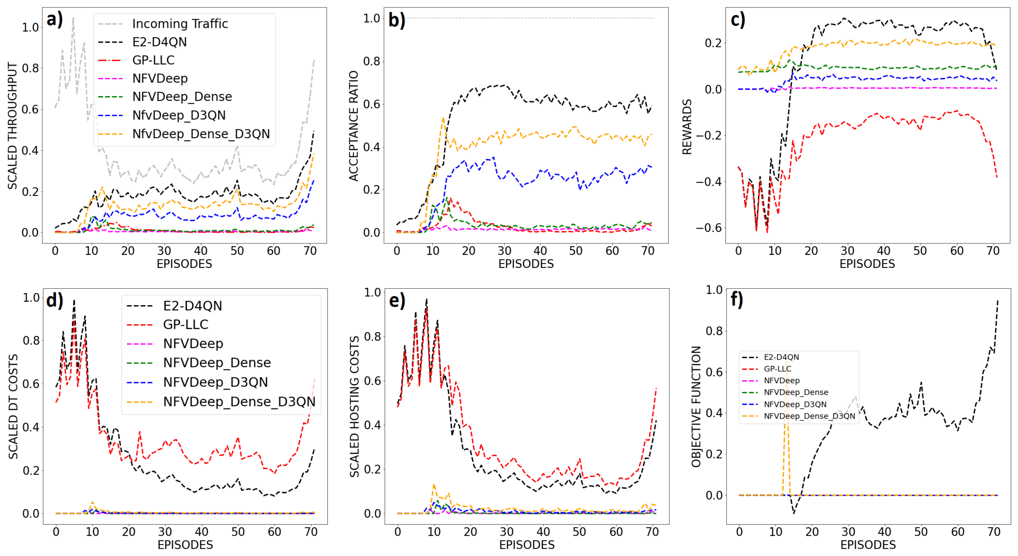
We compare our algorithm with the NFVDeep framework presented in [14]. We have created three progressive enhancements of the NFVDeep algorithm for an exhaustive comparison with E2-D4QN. NFVDeep is a policy gradient DRL framework for maximizing network throughput and minimizing operational costs on general-case SFC deployment. Xiao et al. design a backtracking method: if a resource shortage or exceeded latency event occurs during SFC deployment, the controller ignores the request, and no reward is given to the agent. Consequently, sparse rewards characterize NFVDeep. The first algorithm we compare with is a reproduction of NFVDeep on our particular Live-Streaming vCDN Environment. The second algorithm introduces our dense-reward scheme on the NFVDeep framework, and we call it NFVDeep-Dense. The third method is an adaptation of NFVDeep that introduces our dueling DDQN framework but keeps the same reward policy as the original algorithm in [14], and we call it NFVDeep-D3QN. The fourth algorithm is called NFVDeep-Dense-D3QN, and it adds our dense reward policies to NFVDeep-D3QN. Notice that the difference between NFVDeep-Dense-D3QN and our E2-D4QN algorithm is that the latter does not use the backtracking mechanism: In contrast to any of the compared algorithms, we permit our agent to do wrong VNF assignations and to learn from its mistakes to escape from local optima.

Finally, we also compare our proposed algorithm with a greedy-policy lowest-latency and lowest-cost (GP-LLC) assignation agent, based on the work presented in [57]. GP-LLC is an extension of the algorithm in [57], that includes server-utilization, channel-ingestion state, and resource-costs awareness in the decisions of a greedy policy. For each incoming VNF request, GP-LLC will assign a hosting node. This greedy policy will try not to overload nodes with assignation actions and always choose the best available actions in terms of QoS. Moreover, given a set of candidate nodes respecting such a greedy QoS-preserving criterion, the LLC criterion will tend to optimize hosting costs. Appendix B describes in detail the GP-LLC SFC Deployment algorithm.

3. Results

Various performance metrics for all the algorithms mentioned in Section 2.3.4 are presented in Figure 3. Recall that the measurements in such a figure are taken during the 1-day evaluation trace as mentioned in Section 2.3.2. Notice that, given the time-step duration and number of time-steps per episode specified in Section 2.3.2, one-day trace consists of 72 episodes, starting at 00:00:00 h at finishing at 23:59:59 of the 29 July 2017.

3.1. Mean Scaled Network Throughput per Episode

The network throughput for each simulation time-step was computed using (10) and the mean values for each episode were scaled and plotted in Figure 3a. Also the scaled incoming traffic amount is plotted in such a figure. In the first twenty episodes of the trace, which correspond to the period from 0:00 to 6:00, the incoming traffic goes from intense to moderate. Incoming traffic has minor oscillations with respect to the antecedent descent from episode 20 to episode 60, and it starts to grow again from the sixtieth episode on, which corresponds to the period from 18:00 to the end of the trace.

The initial ten episodes are characterized for a comparable throughput between GP-LLC, E2-D4QN, and NFVDeep-Dense-D3QN. We can see, however, from the 20th episode on, the throughput of policy-based NFVDeep variants is lowered. From episode 15, however, which corresponds to the period from 05:00 to the end of the day, the throughput of our proposed algorithm is superior throughput with respect to every other algorithm.

3.2. Mean Acceptance Ratio per Episode

The AR for each simulation time-step was computed using (1) and the mean values for each episode are plotted in Figure 3b. At the beginning of the test, corresponding to the first five episodes, E2-D4QN has a superior AR performance. From episodes 5 to 15, only E2-D4QN and NFVDeep-Dense-D3QN keep growing in the acceptance ratio. The unique algorithm that holds a satisfactory acceptance ratio during the rest of the day is E2-D4QN instead. It should be stressed that the AR cannot be one in our experiments because the parameter configuration described in Section 2.3.2 resembles overloaded network conditions on purpose.

3.3. Mean Rewards per Episode

Figure 3c shows the mean rewards per episode. We plot the rewards obtained at every $\left|K\right|$ assignation steps. Notice that such a selection corresponds to the non-null rewards in the sparse-reward models.

During the first 15 episodes, -00:00 to 05:00- both GP-LLC and E2-D4QN increment their mean rewards starting from a worse performance with respect to the NFVDeep algorithms. This is explained because the Enhanced-Exploration mechanism of E2-D4QN and GP-LLC is the unique that includes negative rewards in the reward assignation policy. From episode 15 to 20, E2-D4QN reaches the rewards obtained by NFVDeep-Dense-D3QN, and from episode 20 on, E2-D4QN has a better performance with respect to the NFVDeep variants, most of all due to the lowering of operational costs for this algorithm. Finally, with the exception of the last 5 episodes, only E2-D4QN dominates the rest of the trace in the mean reward metric, with the exception of the last five episodes.

3.4. Total Scaled Data-Transportation Costs per Episode

The total DT costs per time-step as defined in (13) were computed and the mean values per episode were scaled and plotted in Figure 3d. During the whole evaluation period, both E2-D4QN and GP-LLC incur higher DT costs with respect to every other algorithm. This phenomenon is explained by the Enhanced Exploration mechanism, which permits E2-D4QN and GP-LLC, to accept requests even when the resulting RTT is over the acceptable threshold. E2-D4QN and GP-LLC accept every incoming request instead. Notice, however, that E2-D4QN and GP-LLC progressively reduce DT costs due to common path creation for similar SFCs.From the twentieth episode on, however, only E2-D4QN minimizes such costs while maintaining an acceptance ratio greater than $0.5$.

3.5. Total Scaled Hosting Costs per Episode

A similar explanation can be given for the total Hosting Cost behavior. Such a cost was computed for each time-step using (11) and the mean values per episode were scaled and plotted in Figure 3e. Given the adaptive resource provisioning algorithm described in Appendix A.1, we can argue that, in general, hosting cost is high for E2-D4QN and GP-LLC because their throughput is high. The hosting costs burst that characterizes the first twenty episodes, however, can be explained by the network initialization state during experiments: Every algorithm is evaluated from an uncommon network state with respect to the steady state reached during training. The algorithms that are equipped with the Enhanced-Exploration mechanism tend to worse such a performance drop at the beginning of the testing trace because of the unconstrained nature of such mechanism. It is the Enhanced-Exploration however, that drives our proposed agent to learn sub-optimal policies that permit to maximize the network acceptance ratio.

3.6. Optimization Objective

The optimization objective as defined in (16) was computed at each time-step, and the mean values per episode were scaled and plotted in Figure 3f. Recall that (16) is invalid whenever the acceptance ratio is above the minimum threshold of 0.5 as mentioned in Section 2.1.4. For this reason, in Figure 3f we set the optimization value to zero whenever the minimum service constraint was not met. Notice that no algorithm can achieve the minimum acceptance ratio during the first ten episodes of the test. This behavior can be explained by the greedy initialization with which every test has been carried out: The initial network state for every algorithm is very different from the states observed during training. From the tenth episode on, however, E2-D4QN is the only algorithm to achieve a satisfactory acceptance ratio, and thus, the optimization objective function has a non-zero value.

4. Discussion

Trace-driven simulations have revealed that our approach shows adaptability to the complexity of the particular context of Live-Streaming in vCDN with respect to the state-of-art algorithms designed for general-case SFC deployment. In particular, our simulation test revealed decisive QoS performance improvements in terms of acceptance ratio with respect to any other backtracking algorithm. Our agent progressively learns to adapt to the complex environment conditions like different user cluster traffic patterns, different channel popularities, unitary resource provision costs, VNF instantiation times, etc.

We assess the algorithm’s performance in a bounded-resource scenario aiming to build a safe-exploration strategy that enables the market entry of new vCDN players. Our experiments have shown that the proposed algorithm, E2-D4QN is the only one to adapt to such conditions, maintaining an acceptance ratio above the general case state-of-art techniques while keeping a delicate balance between network throughput and operational costs.

Based on the results in the previous section, we now argue the main reasons that make E2-D4QN the most suitable algorithm for online optimization of SFC Deployment on a Live-video delivery vCDN scenario. The main reason for our proposed algorithm’s advantage is the combination of the enhanced exploration with a dense-rewards mechanism on a dueling DDQN framework. We argue that such a combination leads to discover convenient long-term actions in contrast to convenient short-term actions during training.

4.1. Environment Complexity Adaptation

As explained in Section 2.3.4, we have compared our E2-D4QN agent with the NFVDeep algorithm presented in [14], with three progressive enhancements to such algorithm, and with an extension of the algorithm presented in [57], which we called GP-LLC. Authors in [14] assumed utilization-independent processing times. A consequence of this assumption is the possibility of computing the remaining latency space with respect to the RTT threshold before each assignment. In our work, instead, we argue that realistic processing times should be modeled as utilization-dependent. Moreover, Xiao et al. did not model ingestion-related utilization nor VNF instantiation time penalties. Relaxing the environment with these assumptions simplifies the environment and helps on-policy DRL schemes like the one in [14] to converge to suitable solutions. Lastly, in NFVDeep, prior knowledge of each SFC session’s duration is also assumed. This feature helps the agent to learn to accept longer sessions to increase the throughput. Unfortunately, it is not realistic to assume session duration knowledge when modeling Live-Streaming in vCDN context. Our model is agnostic to this feature and maximizes the overall throughput when optimizing the acceptance ratio. This paper shows that the NFVDeep algorithm cannot reach a good AR on SFC Deployment optimization without assuming all the aforementioned relaxations.

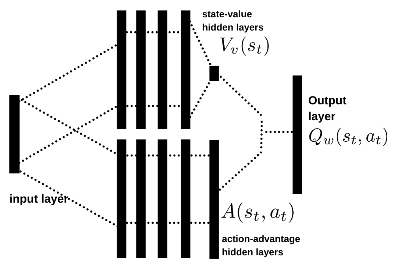
4.2. State Value, Advantage Value and Action Value Learning

In this work, we propose the usage of the dueling-DDQN framework for implementing a DRL agent that optimizes SFC Deployment. Such a framework is meant to learn approximators for the state value function, $V\left(s\right)$, the action advantage function, $A\left(a\right)$, and the action-value function, $Q(s,a)$. Learning such functions helps to differentiate between relevant actions in the presence of many similar-valued actions. This is the main reason why NFVDeep-D3QN improves AR with respect to NFVDeep: Learning the action advantage function, helps to identify convenient long-term actions from a set of similar valued actions. For example, preserving resources of low-cost nodes for popular channel bursts in the future can be more convenient in the long term with respect to adopting a round-robin load-balancing strategy during low incoming traffic periods. Moreover, suppose we do such a round-robin dispatching. In that case, the SFC routes to content providers won’t tend to divide the hosting nodes into non-overlapping clusters. This will provoke more resource usage in the long run: almost every node will ingest the content of almost every content provider. As generally content-ingestion resource usage is much heavier with respect to content-serving, this strategy will accentuate the resource leakage on the vCDN in the long run, provoking bad QoS performance. Our E2-D4QN learns to polarize the SFC routes in order to minimize content ingestion resource usage during the training phase. Such a biased policy performs in the best way possible with respect to the compared algorithms taking into account the whole evaluation period.

4.3. Dense Reward Assignation Policies

Our agent converges to sub-optimal policies by carefully designing a reward schema as the one presented in Section 2.2.2. Our algorithm assigns a specific reward at each MDP transition considering the optimality of VNF assignments in terms of QoS, hosting costs, and data transfer costs. This dense-reward schema enhances the agent’s convergence. In fact, in our experiments, we have also noticed that the dense-reward algorithms improve the results of their sparse-reward counterparts. In other words, we see in Figure 3b that NFVDeep-Dense performs slightly better than NFVDeep, and NFVDeep-Dense-D3QN performs better than NFVDeep-D3QN. This improvement exists because dense rewards provide valuable feedback at each assignation step of the SFC, improving convergence of the DRL agents to shorter RTTs. On the other hand, we have also observed that even if cost-related penalties are sparsely subtracted in our experiments, the proposed DRL agent learns to optimize SFC deployment not only with respect to QoS but also taking into account the operational costs.

4.4. Enhanced Exploration

Notice that GP-LLC does not learn inherent network traffic dynamics, making it impossible to differentiate convenient long-term actions from greedy actions. For example, GP-LLC won’t adopt long-term resource consolidation policies, in which each channel is ingested by a defined subset of nodes to amortize the overall ingestion resource consumption. On the other hand, we argue that the main reason that keeps NFVDeep above a satisfactory performance is the leakage of the enhanced exploration mechanism. In fact, we demonstrate that the acceptance ratio of E2-D4QN surpasses every other algorithm because we add enhanced exploration, which enriches the experience replay buffer with non-optimal SFC deployments during training, preventing the agent from getting stuck at local optima, which we think is the main problem with NVFDeep under our environment conditions.

In practice, in all the NFVDeep or backtracking algorithms, i.e., the algorithms without the enhanced-exploration mechanism, at each VNF assignment, the candidate nodes are filtered based on their utilization availability. Only non-overloaded nodes are available candidates. If the agent chooses an overloaded node, the action is ignored, and no reward is given. Our model instead performs assignment decisions without being constrained by current node utilization to enhance the exploration of the action space. The well-designed state-space codifies important features that drive learning towards sub-optimal VNF placements:

• The request vector codifies useful information about the requests that help our agent extract the incoming traffic patterns.
• The ingestion vector helps our agent to optimize ingestion-related resource demand by avoiding session assignments to VNF instances that do not ingest the content requested at the moment of assignation.
• The maximum utilization vector gives our agent resource utilization awareness, making it able to converge to assignation policies that optimize processing times and preserve QoS.

Consequently, our agent learns optimal SFC Deployment policies without knowing the actual bounds of the resource provision or the current instantiation state of the VNF instances that compose the vCDN. It learns to recognize the maximum resource provisioning for the VNFs and also learns to evict assignations to non-initialized VNFs thanks to our carefully designed reward assignation scheme.

4.5. Work Limitations and Future Research Directions

We have based the experiments in this paper on a real-world data set concerning a particular video delivery operator. In this case, the hosting nodes of the corresponding proprietary CDN are deployed in the Italian territory. However, such a medium-scale deployment is not the unique possible configuration for a CDN. Consequently, as future work, we plan to obtain or generate data concerning high-scale topologies to assess the scalability of our algorithm to such scenarios.

Further, this paper presents the assessment of the performance of various DRL-based algorithms. However, the authors of this work had access to real-world data set limited to a five-day trace. Consequently, the algorithms presented in this work were trained on a four-day trace, while the evaluation period consisted of a single day. Future research directions include assessing our agent’s training and evaluation performance on data concerning more extended periods.

Finally, in this work, we have used a VNF resource-provisioning algorithm that is greedy and reactive, as specified in Appendix A.1. A DRL-based resource-provisioning policy would instead act proactive and long-term convenient actions. Such a resource-provisioning policy, combined with the SFC deployment policy presented in this work, would further optimize QoS and Costs. Thus, future work also includes the development of a multi-agent DRL framework for the joint optimization of both resource provisioning and SFC deployment tasks in the context of live-streaming in vCDN.

References

1. Cisco, V. Cisco Visual Networking Index: Forecast and Methodology 2016–2021. Complet. Vis. Netw. Index (VNI) Forecast. 2017, 12, 749–759. [Google Scholar]
2. Budhkar, S.; Tamarapalli, V. An overlay management strategy to improve QoS in CDN-P2P live streaming systems. Peer-to-Peer Netw. Appl. 2020, 13, 190–206. [Google Scholar] [CrossRef]
3. Demirci, S.; Sagiroglu, S. Optimal placement of virtual network functions in software defined networks: A survey. J. Netw. Comput. Appl. 2019, 147, 102424. [Google Scholar] [CrossRef]
4. Li, J.; Lu, Z.; Tong, Y.; Wu, J.; Huang, S.; Qiu, M.; Du, W. A general AI-defined attention network for predicting CDN performance. Future Gener. Comput. Syst. 2019, 100, 759–769. [Google Scholar] [CrossRef]
5. Yi, B.; Wang, X.; Li, K.; Das, S.k.; Huang, M. A comprehensive survey of Network Function Virtualization. Comput. Netw. 2018, 133, 212–262. [Google Scholar] [CrossRef]
6. Matias, J.; Garay, J.; Toledo, N.; Unzilla, J.; Jacob, E. Toward an SDN-enabled NFV architecture. IEEE Commun. Mag. 2015, 53, 187–193. [Google Scholar] [CrossRef]
7. Taleb, T.; Mada, B.; Corici, M.I.; Nakao, A.; Flinck, H. PERMIT: Network slicing for personalized 5G mobile telecommunications. IEEE Commun. Mag. 2017, 55, 88–93. [Google Scholar] [CrossRef] [Green Version]
8. Khan, R.; Kumar, P.; Jayakody, D.N.K.; Liyanage, M. A Survey on Security and Privacy of 5G Technologies: Potential Solutions, Recent Advancements, and Future Directions. IEEE Commun. Surv. Tutor. 2020, 22, 196–248. [Google Scholar] [CrossRef] [Green Version]
9. Jahromi, N.T. Towards the Softwarization of Content Delivery Networks for Component and Service Provisioning. Ph.D. Thesis, Concordia University, Montreal, QC, Canada, 2018. [Google Scholar]
10. ETSI. ETSI White Paper No. 24, MEC Deployments in 4G and Evolution towards 5G, 02-2018. Available online: https://www.etsi.org/images/files/etsiwhitepapers/etsi_wp24_mec_deployment_in_4g_5g_final.pdf (accessed on 26 October 2021).
11. Hernandez-Valencia, E.; Izzo, S.; Polonsky, B. How will NFV/SDN transform service provider opex? IEEE Netw. 2015, 29, 60–67. [Google Scholar] [CrossRef]
12. Cziva, R.; Pezaros, D.P. Container Network Functions: Bringing NFV to the Network Edge. IEEE Commun. Mag. 2017, 55, 24–31. [Google Scholar] [CrossRef] [Green Version]
13. Herbaut, N.; Negru, D.; Chen, Y.; Frangoudis, P.A.; Ksentini, A. Content Delivery Networks as a Virtual Network Function: A Win-Win ISP-CDN Collaboration. In Proceedings of the 2016 IEEE Global Communications Conference (GLOBECOM), Washington, DC, USA, 4–8 December 2016. [Google Scholar]
14. Xiao, Y.; Zhang, Q.; Liu, F.; Wang, J.; Zhao, M.; Zhang, Z.; Zhang, J. NFVdeep: Adaptive online service function chain deployment with deep reinforcement learning. In Proceedings of the International Symposium on Quality of Service; Number Article 21 in IWQoS ’19; Association for Computing Machinery: New York, NY, USA, 2019; pp. 1–10. [Google Scholar]
15. Lukovszki, T.; Schmid, S. Online Admission Control and Embedding of Service Chains. In Structural Information and Communication Complexity; Springer International Publishing: Berlin/Heidelberg, Germany, 2015; pp. 104–118. [Google Scholar]
16. Huang, W.; Zhu, H.; Qian, Z. AutoVNF: An Automatic Resource Sharing Schema for VNF Requests. J. Internet Serv. Inf. Secur. 2017, 7, 34–47. [Google Scholar]
17. Wowza Media Systems: 4 Tips for Sizing Streaming Server Hardware. 2017. Available online: https://www.wowza.com/blog/4-tips-for-sizing-streaming-server-hardware (accessed on 30 September 2021).
18. Etsi, G. 001, Network Functions Virtualization (NFV): Use Cases, October 2013. Available online: https://www.etsi.org/deliver/etsi_gs/nfv/001_099/001/01.01.01_60/gs_nfv001v010101p.pdf (accessed on 26 October 2021).
19. Herbaut, N. Collaborative Content Distribution over a VNF-as-a-Service Platform. Ph.D. Thesis, Université de Bordeaux, Bordeaux, France, 2017. [Google Scholar]
20. Benkacem, I.; Taleb, T.; Bagaa, M.; Flinck, H. Optimal VNFs Placement in CDN Slicing Over Multi-Cloud Environment. IEEE J. Sel. Areas Commun. 2018, 36, 616–627. [Google Scholar] [CrossRef]
21. Gil Herrera, J.; Botero, J.F. Resource Allocation in NFV: A Comprehensive Survey. IEEE Trans. Netw. Serv. Manag. 2016, 13, 518–532. [Google Scholar] [CrossRef]
22. Fei, X.; Liu, F.; Xu, H.; Jin, H. Adaptive VNF Scaling and Flow Routing with Proactive Demand Prediction. In Proceedings of the IEEE INFOCOM 2018—IEEE Conference on Computer Communications, Honolulu, HI, USA, 16–19 April 2018; pp. 486–494. [Google Scholar]
23. Zhang, R.X.; Ma, M.; Huang, T.; Pang, H.; Yao, X.; Wu, C.; Liu, J.; Sun, L. Livesmart: A QoS-Guaranteed Cost-Minimum Framework of Viewer Scheduling for Crowdsourced Live Streaming. In Proceedings of the 27th ACM International Conference on Multimedia; MM ’19; Association for Computing Machinery: New York, NY, USA, 2019; pp. 420–428. [Google Scholar]
24. Gupta, L.; Jain, R.; Erbad, A.; Bhamare, D. The P-ART framework for placement of virtual network services in a multi-cloud environment. Comput. Commun. 2019, 139, 103–122. [Google Scholar] [CrossRef]
25. Tomassilli, A.; Giroire, F.; Huin, N.; Pérennes, S. Provably Efficient Algorithms for Placement of Service Function Chains with Ordering Constraints. In Proceedings of the IEEE INFOCOM 2018–IEEE Conference on Computer Communications, Honolulu, HI, USA, 16–19 April 2018; pp. 774–782. [Google Scholar]
26. Ibn-Khedher, H.; Abd-Elrahman, E.; Kamal, A.E.; Afifi, H. OPAC: An optimal placement algorithm for virtual CDN. Comput. Netw. 2017, 120, 12–27. [Google Scholar] [CrossRef]
27. Ibn-Khedher, H.; Hadji, M.; Abd-Elrahman, E.; Afifi, H.; Kamal, A.E. Scalable and Cost Efficient Algorithms for Virtual CDN Migration. In Proceedings of the 2016 IEEE 41st Conference on Local Computer Networks (LCN), Dubai, United Arab Emirates, 7–10 November 2016; pp. 112–120. [Google Scholar]
28. Yala, L.; Frangoudis, P.A.; Lucarelli, G.; Ksentini, A. Cost and Availability Aware Resource Allocation and Virtual Function Placement for CDNaaS Provision. IEEE Trans. Netw. Serv. Manag. 2018, 15, 1334–1348. [Google Scholar] [CrossRef]
29. Filelis-Papadopoulos, C.K.; Endo, P.T.; Bendechache, M.; Svorobej, S.; Giannoutakis, K.M.; Gravvanis, G.A.; Tzovaras, D.; Byrne, J.; Lynn, T. Towards simulation and optimization of cache placement on large virtual content distribution networks. J. Comput. Sci. 2020, 39, 101052. [Google Scholar] [CrossRef]
30. Dieye, M.; Ahvar, S.; Sahoo, J.; Ahvar, E.; Glitho, R.; Elbiaze, H.; Crespi, N. CPVNF: Cost-Efficient Proactive VNF Placement and Chaining for Value-Added Services in Content Delivery Networks. IEEE Trans. Netw. Serv. Manag. 2018, 15, 774–786. [Google Scholar] [CrossRef] [Green Version]
31. Jahromi, N.T.; Kianpisheh, S.; Glitho, R.H. Online VNF Placement and Chaining for Value-added Services in Content Delivery Networks. In Proceedings of the 2018 IEEE International Symposium on Local and Metropolitan Area Networks (LANMAN), Washington, DC, USA, 25–27 June 2018; pp. 19–24. [Google Scholar]
32. Jia, Y.; Wu, C.; Li, Z.; Le, F.; Liu, A. Online Scaling of NFV Service Chains Across Geo-Distributed Datacenters. IEEE/ACM Trans. Netw. 2018, 26, 699–710. [Google Scholar] [CrossRef] [Green Version]
33. Das, B.C.; Takahashi, S.; Oki, E.; Muramatsu, M. Approach to problem of minimizing network power consumption based on robust optimization. Int. J. Commun. Syst. 2019, 32, e3891. [Google Scholar] [CrossRef]
34. Xie, Y.; Wang, B.; Wang, S.; Luo, L. Virtualized Network Function Provisioning in Stochastic Cloud Environment. In Proceedings of the ICC 2020—2020 IEEE International Conference on Communications (ICC), Dublin, Ireland, 7–11 June 2020; pp. 1–6. [Google Scholar]
35. Marotta, A.; Kassler, A. A Power Efficient and Robust Virtual Network Functions Placement Problem. In Proceedings of the 2016 28th International Teletraffic Congress (ITC 28), Würzburg, Germany, 12–16 September 2016. [Google Scholar]
36. Marotta, A.; Zola, E.; D’Andreagiovanni, F.; Kassler, A. A fast robust optimization-based heuristic for the deployment of green virtual network functions. J. Netw. Comput. Appl. 2017, 95, 42–53. [Google Scholar] [CrossRef]
37. Ito, M.; He, F.; Oki, E. Robust Optimization Model for Probabilistic Protection under Uncertain Virtual Machine Capacity in Cloud. In Proceedings of the 2020 16th International Conference on the Design of Reliable Communication Networks DRCN 2020, Milan, Italy, 25–27 March 2020. [Google Scholar]
38. Mijumbi, R.; Gorricho, J.; Serrat, J.; Claeys, M.; De Turck, F.; Latré, S. Design and evaluation of learning algorithms for dynamic resource management in virtual networks. In Proceedings of the 2014 IEEE Network Operations and Management Symposium (NOMS), Krakow, Poland, 5–9 May 2014; pp. 1–9. [Google Scholar]
39. Lillicrap, T.P.; Hunt, J.J.; Pritzel, A.; Heess, N.; Erez, T.; Tassa, Y.; Silver, D.; Wierstra, D. Continuous control with deep reinforcement learning. arXiv 2015, arXiv:cs.LG/1509.02971. [Google Scholar]
40. Dulac-Arnold, G.; Evans, R.; van Hasselt, H.; Sunehag, P.; Lillicrap, T.; Hunt, J.; Mann, T.; Weber, T.; Degris, T.; Coppin, B. Deep Reinforcement Learning in Large Discrete Action Spaces. arXiv 2015, arXiv:cs.AI/1512.07679. [Google Scholar]
41. Wang, Z.; Schaul, T.; Hessel, M.; Hasselt, H.; Lanctot, M.; Freitas, N. Dueling Network Architectures for Deep Reinforcement Learning. In Proceedings of Machine Learning Research; PMLR: New York, NY, USA, 2016; Volume 48, pp. 1995–2003. [Google Scholar]
42. Reis, J.; Rocha, M.; Phan, T.K.; Griffin, D.; Le, F.; Rio, M. Deep Neural Networks for Network Routing. In Proceedings of the 2019 International Joint Conference on Neural Networks (IJCNN), Budapest, Hungary, 14–19 July 2019; pp. 1–8. [Google Scholar]
43. Quang, P.T.A.; Hadjadj-Aoul, Y.; Outtagarts, A. A Deep Reinforcement Learning Approach for VNF Forwarding Graph Embedding. IEEE Trans. Netw. Serv. Manag. 2019, 16, 1318–1331. [Google Scholar] [CrossRef] [Green Version]
44. Anh Quang, P.T.; Hadjadj-Aoul, Y.; Outtagarts, A. Evolutionary Actor-Multi-Critic Model for VNF-FG Embedding. In Proceedings of the 2020 IEEE 17th Annual Consumer Communications Networking Conference (CCNC), Las Vegas, NV, USA, 10–13 January 2020; pp. 1–6. [Google Scholar]
45. Yan, Z.; Ge, J.; Wu, Y.; Li, L.; Li, T. Automatic Virtual Network Embedding: A Deep Reinforcement Learning Approach With Graph Convolutional Networks. IEEE J. Sel. Areas Commun. 2020, 38, 1040–1057. [Google Scholar] [CrossRef]
46. Khezri, H.R.; Moghadam, P.A.; Farshbafan, M.K.; Shah-Mansouri, V.; Kebriaei, H.; Niyato, D. Deep Reinforcement Learning for Dynamic Reliability Aware NFV-Based Service Provisioning. In Proceedings of the 2019 IEEE Global Communications Conference (GLOBECOM), Waikoloa, HI, USA, 9–13 December 2019; pp. 1–6. [Google Scholar]
47. Mao, W.; Wang, L.; Zhao, J.; Xu, Y. Online Fault-tolerant VNF Chain Placement: A Deep Reinforcement Learning Approach. In Proceedings of the 2020 IFIP Networking Conference (Networking), Paris, France, 22–26 June 2020; pp. 163–171. [Google Scholar]
48. Pei, J.; Hong, P.; Pan, M.; Liu, J.; Zhou, J. Optimal VNF Placement via Deep Reinforcement Learning in SDN/NFV-Enabled Networks. IEEE J. Sel. Areas Commun. 2020, 38, 263–278. [Google Scholar] [CrossRef]
49. Santos, G.L.; Kelner, J.; Sadok, D.; Endo, P.T. Using Reinforcement Learning to Allocate and Manage SFC in Cellular Networks. In Proceedings of the 2020 16th International Conference on Network and Service Management (CNSM), Izmir, Turkey, 2–6 November 2020; pp. 1–5. [Google Scholar]
50. Beck, M.T.; Botero, J.F. Coordinated Allocation of Service Function Chains. In Proceedings of the 2015 IEEE Global Communications Conference (GLOBECOM), San Diego, CA, USA, 6–10 December 2015; pp. 1–6. [Google Scholar]
51. Pei, J.; Hong, P.; Xue, K.; Li, D. Resource Aware Routing for Service Function Chains in SDN and NFV-Enabled Network. IEEE Trans. Serv. Comput. 2018, 14, 985–997. [Google Scholar] [CrossRef]
52. Pei, J.; Hong, P.; Xue, K.; Li, D. Efficiently Embedding Service Function Chains with Dynamic Virtual Network Function Placement in Geo-Distributed Cloud System. IEEE Trans. Parallel Distrib. Syst. 2019, 30, 2179–2192. [Google Scholar] [CrossRef]
53. Mnih, V.; Kavukcuoglu, K.; Silver, D.; Graves, A.; Antonoglou, I.; Wierstra, D.; Riedmiller, M. Playing Atari with Deep Reinforcement Learning. arXiv 2013, arXiv:cs.LG/1312.5602. [Google Scholar]
54. Mnih, V.; Kavukcuoglu, K.; Silver, D.; Rusu, A.A.; Veness, J.; Bellemare, M.G.; Graves, A.; Riedmiller, M.; Fidjeland, A.K.; Ostrovski, G.; et al. Human-level control through deep reinforcement learning. Nature 2015, 518, 529–533. [Google Scholar] [CrossRef]
55. van Hasselt, H.; Guez, A.; Silver, D. Deep Reinforcement Learning with Double Q-learning. arXiv 2015, arXiv:cs.LG/1509.06461. [Google Scholar]
56. Hasselt, H. Double Q-learning. Adv. Neural Inf. Process. Syst. 2010, 23, 2613–2621. [Google Scholar]
57. Sun, C.; Bi, J.; Zheng, Z.; Hu, H. SLA-NFV: An SLA-aware High Performance Framework for Network Function Virtualization. In Proceedings of the 2016 ACM SIGCOMM Conference; SIGCOMM ’16; Association for Computing Machinery: New York, NY, USA, 2016; pp. 581–582. [Google Scholar]
Figure 1. The assumed Service Function Chain composition for every Live-Video Streaming session request. We assume that every incoming session needs for a streamer, a compressor a transcoder and a cache VNF modules. We assume container based virtualization of a vCDN.
Futureinternet 13 00278 g001
Figure 2. Dueling-architectured DDQN topology for our SFC Deployment agent: A two-stream deep neural network. One stream approximates the state-value function, and the other approximates the action advantage function. These values are combined to get the state-action value estimation in the output layer. The inputs are instead the action is taken and the current state.
Futureinternet 13 00278 g002
Figure 3. Basic evaluation metrics of E2-D4QN, GP-LLC, NFVDeep and three variants of the latter, presented in Section 2.3.4. (a) Scaled mean network throughput per episode. (b) Mean Acceptance Ratio per episode. (c) Mean rewards per episode. (d) Mean scaled total Data-Transportation Costs per episode (e) Mean scaled total hosting costs per episode. (f) Mean scaled optimization objective per episode.
Futureinternet 13 00278 g003