Article

Automatic Addition of Fault-Tolerance in Presence of Unchangeable Environment Actions

by
Mohammad Roohitavaf
*,‡ and
Sandeep Kulkarni
*,‡
Department of Computer Science and Engineering, Michigan State University, East Lansing, MI 48824, USA
*
Authors to whom correspondence should be addressed.
This paper is an extended version of our paper: Roohitavaf, M.; Kulkarni, S. Stabilization and fault-tolerance in presence of unchangeable environment actions. In Proceedings of the 17th International Conference on Distributed Computing and Networking, Singapore, Singapore 4–7 January 2016; p. 19.
These authors contributed equally to this work.
Future Internet 2019, 11(7), 144; https://doi.org/10.3390/fi11070144
Submission received: 15 April 2019 / Revised: 24 June 2019 / Accepted: 28 June 2019 / Published: 4 July 2019
(This article belongs to the Special Issue Dependable Cyber Physical Systems)

Abstract

:
We focus on the problem of adding fault-tolerance to an existing concurrent protocol in the presence of unchangeable environment actions. Such unchangeable actions occur in cases where a subset of components/processes cannot be modified since they represent third-party components or are constrained by physical laws. These actions differ from faults in that they are (1) simultaneously collaborative and disruptive, (2) essential for satisfying the specification and (3) possibly non-terminating. Hence, if these actions are modeled as faults while adding fault-tolerance, it causes existing model repair algorithms to declare failure to add fault-tolerance. We present a set of algorithms for adding stabilization and fault-tolerance for programs that run in the presence of environment actions. We prove the soundness, completeness and the complexity of our algorithms. We have implemented all of our algorithms using symbolic techniques in Java. The experimental results of our algorithms for various examples are also provided.

1. Introduction

Model repair is the problem of revising an existing model/program so that it satisfies new properties while preserving existing properties. It is desirable in several contexts such as when an existing program needs to be deployed in a new setting or to repair bugs. Model repair for fault-tolerance enables one to separate the fault-tolerance and functionality so that the designer can focus on the functionality of the program and utilize automated techniques for adding fault-tolerance. It can also be used to add fault-tolerance against a newly discovered fault.
This paper focuses on performing such repair when some actions cannot be removed from the model. We refer to such transitions as unchangeable environment actions. There are several possible reasons for actions being unchangeable. Examples include scenarios where the system consists of several components –some of which are developed in-house and can be repaired and some of which are third-party and cannot be changed. They are also useful in systems such as Cyber-Physical Systems (CPS) where modifying physical components may be very expensive or even impossible.
The environment actions differ from fault actions considered in existing work such as [1]. Fault actions are assumed to be temporary in nature and all the previously proposed algorithms to add fault-tolerance in [1] work only with this important assumption that faults finally stop occurring. Unlike fault actions, environment actions can keep occurring. Environment actions also differ from adversary actions considered in [2] or in the context of security intrusions. In particular, the adversary intends to cause harm to the system. By contrast, environment actions can be collaborative as well. In other words, environment actions are simultaneously collaborative and disruptive. The goal of this work is to identify whether it is possible for the program to be repaired so that it can utilize the assistance provided by the environment while overcoming its disruption. To give an intuition of the role of the environment and the difference between program, environment and fault actions, we present the following examples.
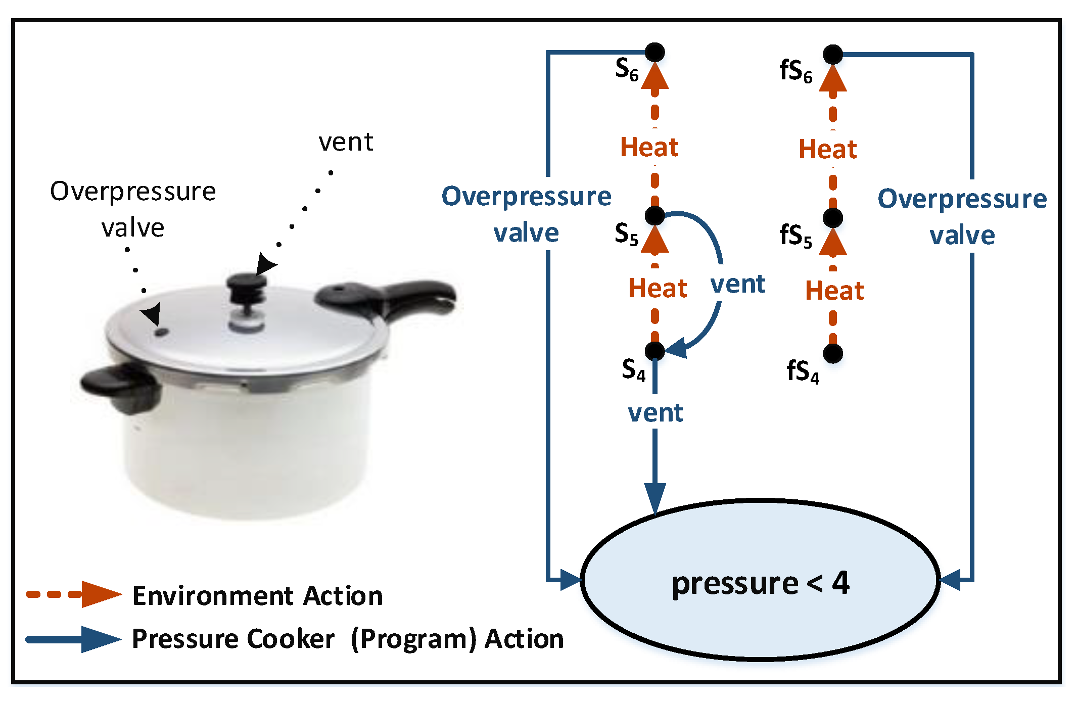
Intuitive examples to illustrate the role of the environment. The first intuitive example is motivated by a simple pressure cooker (see Figure 1). The environment (heat source) causes the pressure to increase. In the subsequent discussion, we analyze this pressure cooker when the heat source is always on. There are two mechanisms to decrease the pressure, a vent and an overpressure valve. For the sake of presentation, assume that pressure below 4 is normal. If the pressure increases to 4 or 5, the vent mechanism reduces the pressure by 1 in each step. However, the vent may fail (e.g., if something gets stuck in the vent pipe) and its pressure reduction mechanism becomes disabled. If the pressure reaches 6, the overpressure valve mechanism causes the valve to open resulting in an immediate drop in pressure to be less than 4. We denote the state where the pressure is x by s x when the vent is working and by f s x when the vent has failed.
Our goal in the subsequent discussion is to model the pressure cooker as a program and identify an approach for the role of the environment and its interaction with the program so that we can conclude this requirement: starting from any state identified above, the system reaches a state where the pressure is less than 4.
Next, we argue that how the role of the environment differs from the role of fault and program actions. In turn, this prevents us from using existing approaches such as Reference [1]. Specifically,
  • Treating the environment as a fault does not work. Faults are assumed to be exceptional events in the system that are expected to stop after some time. By contrast, heat is an essential part of the system that is needed for the system to work. In addition, if we treat the environment as a fault, then none of the environment transitions including transitions from state f s 4 to f s 5 and from f s 5 to f s 6 are required to occur. If these actions do not occur, the overpressure valve is never activated. Hence, neither the valve nor the vent mechanism reduces the pressure to be less than 4.
  • Treating the environment transitions similar to program transitions is also not acceptable. To illustrate this, consider the case where we want to make changes to the program in Figure 1. For instance, if the overpressure valve is removed, then this would correspond to removing the transition from s 6 (respectively f s 6 ) to where the pressure is less than 4. Also, if we add another safety mechanism, it would correspond to adding new transitions. However, we cannot do the same with environment actions that capture the changes made by the heat source. For example, we cannot add new transitions (e.g., from f s 4 to s 4 ) to the environment and we cannot remove transitions (e.g., from s 4 to s 5 ). In other words, even if we make any changes to the model in Figure 1 by adding or removing safety mechanisms, the transitions marked as environment actions remain unchanged. We cannot introduce new environment transitions and we cannot remove existing environment transitions. This is what we mean by the environment being unchangeable.
  • Treating the environment to be collaborative without some special fairness to the program does not work either. In particular, without some special fairness for the program, the system can cycle through states s 4 , s 5 , s 4 , s 5 .
  • Treating the environment to be simultaneously collaborative as well as adversarial where the program has some special fairness enables one to ensure that this program achieves its desired goals. In particular, we need the environment to be collaborative, that is, if it reaches a state where only environment actions can execute then one of them execute This is necessary to ensure that system can transition from state f s 4 to f s 5 and from f s 5 to f s 6 which is essential for recovery to a state where the pressure is less than 4. We also need the program to have special fairness to require that it executes faster than the environment so that it does not execute in a cycle through states s 4 , s 5 , s 4 , (we will precisely define the notion of faster in Section 2.1).
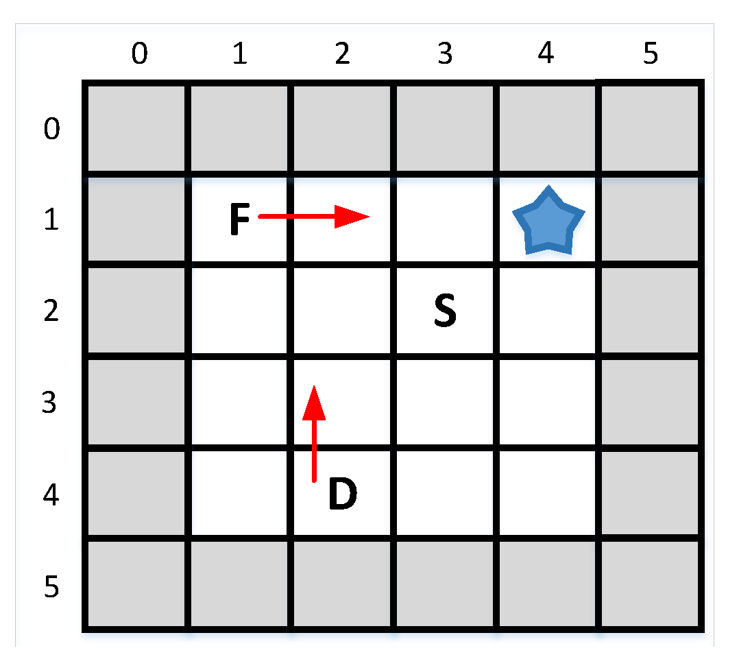
As another example, consider the shepherding problem. In this problem, a shepherd and his dog want to steer a sheep to a specific location (cf. Figure 2). They cannot carry the sheep; the only way to move the sheep is the movement of the sheep by itself. The sheep always tries to increase its distance from the shepherd and the dog. In this example, the program captures the behavior of the shepherd and the dog and the environment captures the behaviors of the sheep.
Like the pressure cooker example, the environment is both assistive and disruptive. On one hand, the environment is assistive, because without the environment actions it is impossible to reach the desired state. On the other hand, the environment is disruptive, because the environment actions can make a (poorly designed) program go into an infinite loop thereby never reaching the desired state. A good program, however, uses the assistance of the sheep (i.e., the environment) while overcomes its disruption to steer the sheep to the desired location.
Goal of the paper. Based on the above examples, our goal in this paper is to evaluate how such simultaneously collaborative and adversarial environment can be used in adding stabilization and fault-tolerance to a given program.
A preliminary version of this work appeared in [3]. In addition to the results presented in [3], in this paper, we provide a sound and complete algorithm for adding masking fault-tolerance. We also introduce our JavaRepair package that includes implementation of our algorithms in Java using symbolic techniques to support larger state spaces. We provide experimental results of using our proposed algorithms to solve different versions of the shepherding problem. To obtain these results, we have used our JavaRepair package. The main results of this work are as follows:
  • We formalize definitions and problems statements for the addition of stabilization and fault-tolerance in presence of unchangeable environment actions.
  • We present an algorithm for the addition of stabilization to an existing program. This algorithm is sound and complete, that is, the program found by it is guaranteed to be stabilizing and if it declares failure then it implies that adding stabilization to that program is impossible.
  • We present a sound and complete algorithm for the addition of fail-safe fault-tolerance.
  • We present a sound and complete algorithm for the addition of masking fault-tolerance.
  • We show that the complexity of all algorithms presented in this paper is polynomial (in the state space of the program).
  • We present our JavaRepair package that includes the implementation of the algorithms presented in this paper available at [4].
  • We present experimental results of applying our algorithms for different examples.
Organization of the paper. This paper is organized as follows: in Section 2, we provide the definitions of a program, environment, specification, fault, fault-tolerance and stabilization. In Section 3 we define the problem of adding stabilization and propose an algorithm to solve that problem. In Section 4, as a case study, we illustrate how the proposed algorithm can be used for a smart grid controller. In Section 5, we define the problem of adding fault-tolerance and propose algorithms to add failsafe and masking fault-tolerance. In Section 6, we present our JavaRepir package and provide experimental results for several examples. In Section 7, we show how our proposed algorithms can be extended to solve related problems. In Section 8, we discuss related work. Finally, we make concluding remarks in Section 9.

2. Preliminaries

In this section, we define the notion of program, environment, specification, fault and fault-tolerance. The definition of the specification is based on the definition by Alpern and Schneider [5]. The definitions of fault and fault-tolerance are adapted from those by Arora and Gouda [6].

2.1. Program Design Model

We define a program in terms of its states and transitions. Intuitively, the state space of a program represents the set of all possible states that a program can be in. On the other hand, transitions specify how the program moves from one state to another.
Definition 1 (Program).
A program p is a tuple S p , δ p where S p is the state space of program p and δ p S p × S p .
In addition to program transitions, the state of a program may change due to the environment where the program is running. Instead of modeling the environment in terms of concepts such as variables that are written by program and variables that are written by the environment, we use a more general approach which models it as a set of transitions that is a subset of S p × S p .
Definition 2 (Environment).
An environment δ e for program p, is defined as a subset of S p × S p .
Our algorithms assume that from any state in the state space of a program p in an environment δ e , there is at least one transition in δ p δ e . If there is no transition from state s 0 in δ p δ e of the given program, we add the self-loop transition ( s 0 , s 0 ) to δ p . We note that this assumption is not restrictive. Instead, it is made to simplify subsequent definitions, since we do not need to concern with terminating computations separately.
We refer to a subset of states of a program by a state predicate. Thus, we have
Definition 3 (State Predicate).
A state predicate of p is any subset of S p .
Note that we can represent a state predicate by either a subset of states or a predicate. Thus, there is a correspondence between a state predicate and subset of states where the state predicate is true. For example, state predicate T r u e is a subset that includes all states of a program and F a l s e is an empty set. Similarly, the negation of a state predicate is the set of states where the given state predicate is false. We say a state predicate is closed in a set of transitions if no transition in the set leaves the state predicate.
Definition 4 (Closure).
A state predicate S is closed in a set of transitions δ iff ( ( s 0 , s 1 ) : ( s 0 , s 1 ) δ : ( s 0 S s 1 S ) ) . (We use Q x : D ( x ) : P ( x ) to specify a formula where Q x is a quantifier that is instantiated to be x or x , D ( x ) is a domain where x can come from and P ( x ) is predicate over x. When there is no restriction on the domain, we use Q : : P . For example, ‘ x : x is odd: x is prime’ states that there exists an x in { 1 , 3 , 5 , } that is a prime.)
Definition 5 (Projection).
The projection of a set of transition δ on state predicate S, denoted as δ | S , is set { ( s 0 , s 1 ) : ( s 0 , s 1 ) δ s 0 , s 1 S } . In other words, δ | S consists of transitions of δ that start at S and end in S.
A computation of a program in an environment is a sequence of states that starts in an initial state and in each state executes either a program transition or an environment transition. Moreover, after an environment transition executes, the program is given a chance to execute in the next k 1 steps. However, whenever in a state no program transition is available, an environment transition can execute.
Definition 6 (p[]kδe computation).
Let p be a program with state space S p and transitions δ p . Let δ e be an environment for program p and k be an integer greater than 1. We say that a sequence σ = s 0 , s 1 , s 2 , is a p [ ] k δ e computation iff
  • i : i 0 : s i S p , and
  • i : i 0 : ( s i , s i + 1 ) δ p δ e , and
  • i : i 0 : ( ( s i , s i + 1 ) δ e )
    ( l : i < l < i + k : ( s l : : ( s l , s l ) δ p ) ( s l , s l + 1 ) δ p ) ) .

2.2. Specification

Following Alpern and Schneider [5], we let the specification of the program consist of a safety specification and a liveness specification. The safety specification identifies bad things that the program should not do. We define a safety specification as a set of (bad) transitions. Specifically,
Definition 7 (Safety).
A safety property is specified in terms of a set of bad transitions, δ b , that the program is not allowed to execute. Thus, a sequence σ = s 0 , s 1 , satisfies the safety property δ b iff j : j > 0 : ( s j , s j + 1 ) δ b .
Liveness, on the other hand, identifies good things that the program should do. We define a liveness property in terms of a set of leads-to properties. A leads-to property is of the form L T where L and T are two state predicates and the leads-to property requires that if the program reaches a state in L it eventually reaches a state in T. Specifically,
Definition 8 (Leads-to).
A leads-to property is specified in terms of L T , where both L and T are state predicates. A sequence σ = s 0 , s 1 , satisfies the leads-to property iff j : s j L : ( k : k j : s k T ) .
Finally, a specification consists of a safety property and a liveness specification (in terms of a set of leads-to properties).
Definition 9 (Specification).
A specification s p e c , is a tuple S f , L v , where S f is a safety property and L v is a set of leads-to properties. A sequence σ satisfies s p e c iff it satisfies S f and L v .
Definition 10 (Satisfaction).
Program p k-satisfies specification s p e c from S in environment δ e iff the following conditions hold:
  • S is closed in δ p δ e , and
  • Every p [ ] k δ e computation that starts from a state in S satisfies s p e c .
We note that from the above definition, it follows that starting from a state in S, execution of either a program transition or an environment transition results in a state in S. Transitions that start from a state in S and reach a state outside S will be modeled as faults (cf. Definition 12). We define an invariant for a program as a subset of states such that if the program starts from that subset, it satisfies its required specification.
Definition 11 (Invariant).
State predicate S is an invariant of p for specification s p e c iff
  • S , and
  • p k-satisfies s p e c from S.

2.3. Faults and Fault-Tolerance

Like environment transitions, we define a class of faults for a program as a set of transitions that may change the state of the program:
Definition 12 (Fault).
A class of faults f for p ( = S p , δ p ) is a subset of S p × S p .
Now, we extend Definition 6 to one that captures the computation of a program in presence of fault transitions:
Definition 13 (p[]kδe[]f computation).
Let p be a program with state space S p and transitions δ p . Let δ e be an environment for program p, k be an integer greater than 1 and f be the set of faults for program p. We say that a sequence σ = s 0 , s 1 , s 2 , is a p [ ] k δ e [ ] f computation iff
  • i : i 0 : s i S p , and
  • i : i 0 : ( s i , s i + 1 ) δ p δ e f , and
  • i : i 0 : ( s i , s i + 1 ) δ e
    l : i < l < i + k : ( s l : : ( s l , s l ) δ p ( s l , s l + 1 ) ( δ p f ) ) , and
  • n : n 0 : ( j : j > n : ( s j 1 , s j ) ( δ p δ e ) ) .
Note that in the above definition, we require that fault transitions finally stop occurring. This captures the transient nature of faults. On the other hand, environment transitions keep occurring forever. Fault transitions can perturb the program by arbitrarily changing its state. The definition of fault-span captures the boundary up to which the program could be perturbed by faults. Thus,
Definition 14 (Fault-span).
The state predicate T is a k-f-span of p from S in environment δ e iff
  • S T , and
  • for every p [ ] k δ e [ ] f computation s 0 , s 1 , s 2 , , where s 0 S , i : s i T .
Next, we define the notion of fault-tolerance. We consider two different types of fault-tolerance namely failsafe and masking fault-tolerance. A failsafe fault-tolerance ensures that the safety property of the desired specification (cf. Definition 9) is not violated even if faults occur. In other words, we have
Definition 15 (Failsafe fault-tolerance).
Program p is failsafe k-f-tolerant to specification s p e c (= S f , L v ) from S in environment δ e iff the following two conditions hold:
  • p k-satisfies s p e c from S in environment δ e and
  • any prefix of any p [ ] k δ e [ ] f computation that starts from S satisfies S f .
Masking fault-tolerance is stronger than failsafe fault-tolerance, as in addition to satisfying the safety property, masking fault-tolerance requires recovery to the invariant. Specifically,
Definition 16 (Masking fault-tolerance).
p is masking k-f-tolerant to specification s p e c from S in environment δ e iff the following two conditions hold:
  • p is failsafe k-f-tolerant to s p e c (= S f , L v ) from S in environment δ e and
  • there exists T such that (1) T is an k-f-span of p from S in environment δ e and (2) for every p [ ] k δ e [ ] f computation σ ( = s 0 , s 1 , s 2 , ) that starts from a state in S, for any i such that s i T , then there exists j i such that s j S .
The second constraint in Definition 16 simply means that in any computation that starts at T must go to S.
We also define the notion of stabilizing programs. We extend the definition from References [7] and [8] for a program in the presence of environment actions.
Definition 17 (Stabilization).
Program p is k-stabilizing for invariant S in environment δ e , iff following conditions hold:
  • S is closed in δ p δ e , and
  • for any p [ ] k δ e computation s 0 , s 1 , s 2 , . . there exists l such that s l S .

3. Addition of Stabilization

In this section, we present our algorithm for adding stabilization to an existing program. In Section 3.1, we identify the problem statement and in Section 3.2, we present an algorithm to add stabilization. Finally, in Section 3.3, we provide proofs of soundness, completeness and the complexity results of the proposed algorithm.

3.1. Problem Definition

The problem of adding of stabilization begins with a program p = S p , δ p , its invariant S and an environment δ e . The goal is to change the set of program transitions so that starting from an arbitrary state, the program recovers to S. In addition, we do not want to change the behavior of the program inside its invariant. Thus, during the addition, we are not allowed to change the set of program transitions in the invariant (i.e., δ p | S ). Also, we introduce parameter δ r that identifies additional restrictions on program transitions. As an example, consider the case where a program cannot change the value of a sensor, that is, it can only read it. However, the environment can change the value of the sensor. In this case, transitions that change the value of the sensor are disallowed as program transitions but they are acceptable as environment transitions. Thus, the problem statement is as follows:
Given program p with state space S p and transitions δ p , invariant S, environment δ e , set of program restriction δ r and k > 1 , identify p with state space S p such that:
C1 
p | S = p | S
C2 
p is k-stabilizing for invariant S in the environment δ e .
C3 
δ p δ r =

3.2. Algorithm to Add Stabilization

The algorithm proposed here adds stabilization for the case where k = 2 . When k = 2 , environment transitions can execute immediately after any program transition. By contrast, for larger k, the environment transitions may have to wait until the program has executed k 1 transitions.
The procedure for adding stabilization is as shown in Algorithm 1. In this algorithm, δ p is the set of transitions of the final stabilizing program. Inside the invariant, the transitions must be equal to the original program (Constraint C1). Therefore, in the first line, we set δ p to δ p | S . Next, the algorithm expands set R that includes states from which all computations reach a state in S. Initially, R is set to S at (Line 2).
State predicate R p is the set of states that can reach a state in R using an unrestricted program transition, that is, a transition not in δ r . In each iteration, R p is the set of new states that we add to R p . In Line 9, we add program transitions from states in R p to states in R to δ p .
Algorithm 1 Addition of stabilization
Input: 
S p , δ p , δ e , S , and δ r
Output: 
δ p or Not-Possible
1:
δ p : = ( δ p | S ) ;
2:
R = S ;
3:
R p = { }
4:
repeat
5:
R = R ;
6:
R p = { s 0 | s 0 ( R R p ) s 1 : s 1 R : ( s 0 , s 1 ) δ r } ;
7:
R p = R p R p ;
8:
for e a c h s 0 R p do
9:
   δ p = δ p { ( s 0 , s 1 ) | ( s 0 , s 1 ) δ r s 1 R } ;
10:
end for
11:
for e a c h s 0 R : s 2 ¬ ( R R p ) : ( s 0 , s 2 ) δ e ( s 1 : s 1 ( R R p ) : ( s 0 , s 1 ) δ e s 0 R p ) do
12:
   R = R s 0 ;
13:
end for
14:
until ( R = R ) ;
15:
if s 0 R then
16:
return Not-Possible;
17:
else
18:
return δ p ;
19:
end if
In the loop on Lines 11–13, we add more states to R. We add s 0 to R (Line 12), whenever every computation starting from s 0 has a state in S. A state s 0 can be added to R only when there is no environment transition starting from s 0 going to a state outside R R p . In addition to this condition, there must be at least one transition from s 0 that reaches R. The loop on Lines 4–14 terminates if no state is added to R in an iteration. Upon termination of the loop, the algorithm declares failure to add stabilization if there exists a state outside R. Otherwise, it returns δ p as the set of transitions of the stabilizing program.
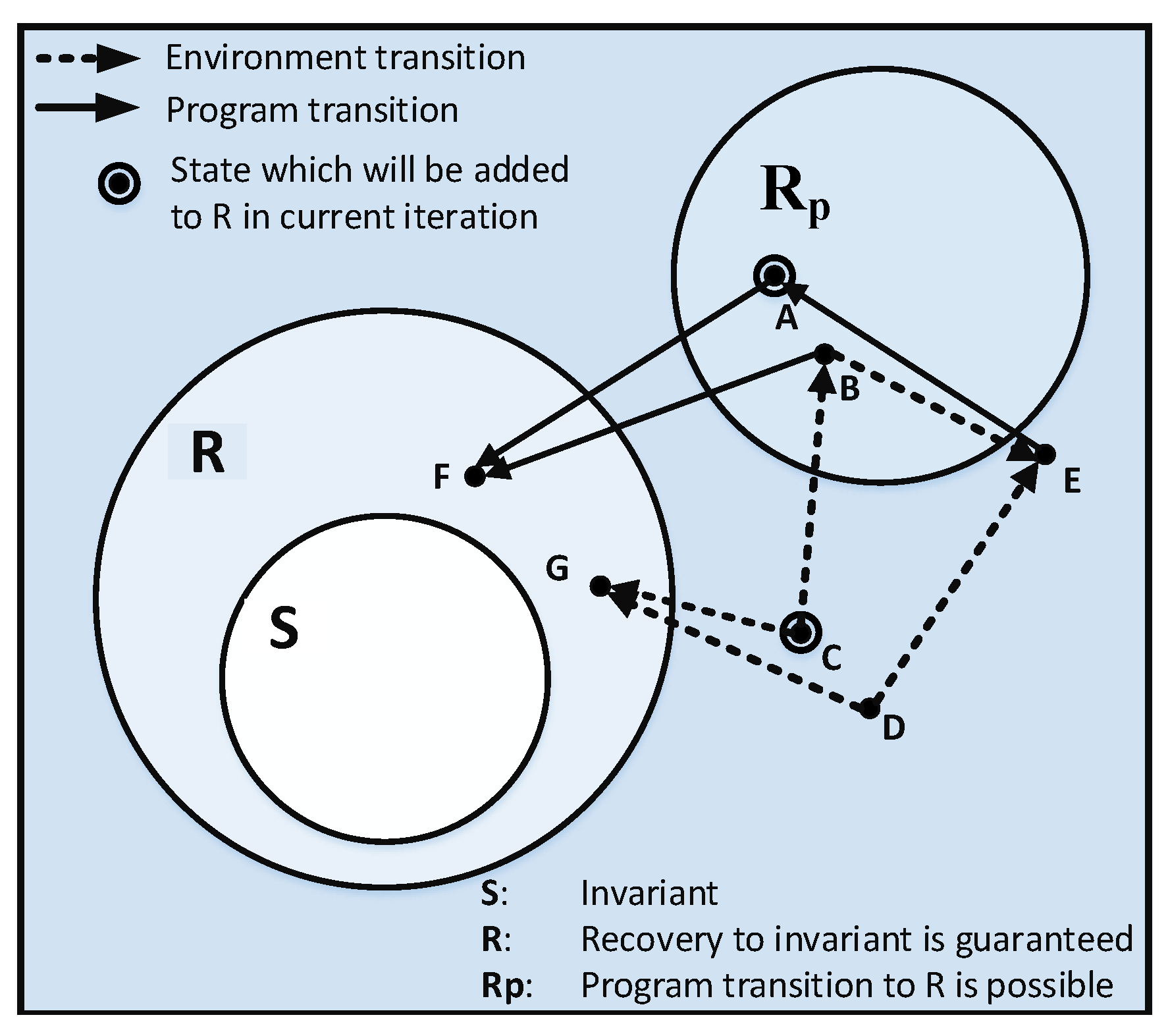
We use Figure 3 as an example to illustrate Algorithm 1. Figure 3 depicts the status of the state space in a hypothetical ith iteration of the loop on Lines 4–14. In this iteration, state A is added to R. This is due to the fact that (1) there is at least one transition from A (namely ( A , F ) ) that reaches R and (2) there is no environment transition from A that reaches outside R R p . Likewise, state C is also added to R. State B is not added to R due to environment transition ( B , E ) . Likewise, state D is not added to R. State E is not added to R since there is no transition from E to a state in R.
In the next, that is, ( i + 1 ) th iteration, E is added to R due to transition ( E , A ) that goes to A that was added to R in the ith iteration. Continuing this, B and D will be added in the ( i + 2 ) th iteration.

3.3. Soundness, Completeness and Complexity Results

In this Section, we show that Algorithm 1 is sound and complete and its time complexity is polynomial in the size of the state space.
Soundness: First, we show that Algorithm 1 is sound, that is, if it finds a solution, the solution satisfies the problem statement for adding stabilization provided in Section 3.1.
Based on the notion of fairness for program transitions, we introduce the notion of whether an environment transition can execute in a given computation prefix. An environment transition can execute in a computation prefix if an environment transition exists in the last state of the prefix and either (1) there are no program transitions starting from the last state of the prefix or (2) the last k 1 transitions of the prefix are program transitions.
Definition 18 (Environment-enabled).
In any prefix of any p [ ] k δ e computation σ = s 0 , s 1 , , s i , s i is an environment-enabled state iff
( s : : ( s i , s ) δ e ) ( s i , s ) : : ( s i , s ) δ p j : j > i k : ( s j , s j + 1 ) δ e .
The following lemma focuses on the recovery to S from states in R:
Lemma 1.
Any p [ ] k δ e computation that starts from a state in R, contains a state in S.
Proof. 
We prove this by induction.
Base case: R = S . The statement is satisfied trivially.
Induction hypothesis: Theorem holds for the current set of R.
Induction step: We show when we add a state to R, the theorem still hold for R. A state s 0 is added to R in two cases:
Case 1 ( s 2 : s 2 ¬ ( R R p ) : ( s 0 , s 2 ) δ e ) ( s 1 : s 1 ( R R p ) : ( s 0 , s 1 ) δ e )
Since there is no s 2 in ¬ ( R R p ) such that ( s 0 , s 2 ) δ e , for every ( s 0 , s 1 ) δ e , s 1 is in R R p . In addition, we know that there is at least one s 1 in R R p such that ( s 0 , s 1 ) δ e . By the construction of R p , we know that if s 1 is in R p , there is a program transition from s 1 to a state in R. Since ( s 0 , s 1 ) δ e and because of the fairness assumption, the program can occur and reach R. Thus, every computation starting from s 0 has a state in R. Since we do not change the set of transitions of states in R of the previous iteration, the set of computations starting from any state in R is unchanged. Thus, based on the induction hypothesis, every computation starting from s 0 has a state in S.
Case 2 s 2 : s 2 ¬ ( R R p ) : ( s 0 , s 2 ) δ e s 0 R p
Since there is no s 2 in ¬ ( R R p ) such that ( s 0 , s 2 ) δ e , for every ( s 0 , s 1 ) δ e , s 1 is either in R or R p . In addition, we know that there is at least one state s 3 in R such that ( s 0 , s 3 ) δ p . In any p [ ] k δ e computation starting from s 0 if ( s 0 , s 1 ) δ p then s 1 R . If ( s 0 , s 1 ) δ e then s 1 R R p . By construction of R p , we know that if s 1 is in R p , there is a program transition from s 1 to a state in R. Since ( s 0 , s 1 ) δ e and because of the fairness assumption, program can reach R. Thus, every computation starting from s 0 has a state in R. Since we do not change the set of transitions of states in R of the previous iteration, the set of computations starting from any state in R is unchanged. Thus, based on the induction hypothesis, every computation starting from s 0 has a state in S. □
Theorem 1.
Algorithm 1 is sound.
Proof. 
We need to show that the constraints of the problem definition are satisfied. At the beginning of the algorithm δ p = δ p | S and all other transitions added to δ p in the rest of the algorithm starts outside S. Thus, p | S = p | S that satisfies the first constraint. The second constraint is satisfied based on Lemma 1 and the fact that R includes all states. The third constraint is satisfied, as we do not add any transitions in δ r to the program. □
Completeness: Next, we focus on showing that Algorithm 1 is complete, that is, if there is a solution that satisfies the problem statement for adding stabilization, Algorithm 1 finds one. The proof of completeness is based on the analysis of states that are not in R upon termination.
Any state that is not in R at the end of Algorithm 1, either does not have any environment transition, or it has an environment transition that goes to ¬ ( R R p ) . Thus, we note the following observation:
Observation 1.
For any s 0 such that s 0 R and s 1 : : ( s 0 , s 1 ) δ e , we have s 2 : s 2 ¬ ( R R p ) : ( s 0 , s 2 ) δ e .
Also, if a state is in R p but it is not in R, it has an environment transition to ¬ ( R R p ) .
Observation 2.
For any s 0 ¬ R R p , s 1 : s 1 ¬ ( R R p ) : ( s 0 , s 1 ) δ e .
Now, for the rest of our discussion in this section, we assume that Algorithm 1 has returned failure. The following lemma focuses on the situation where a given revision p reaches a state marked as ¬ ( R R p ) by Algorithm 1.
Lemma 2.
Let δ p be any program such that δ p δ r = . Let s j be any state in ¬ ( R R p ) at the end of Algorithm 1. Then, for every p [ ] k δ e prefix α = , s j 1 , s j , there exists suffix β = s j + 1 , s j + 2 , , such that α β is a p [ ] k δ e computation and one of two conditions below is correct:
1. 
s j + 1 ¬ ( R R p )
2. 
s j + 1 ( R p R ) s j + 2 ¬ ( R R p )
Proof. 
There are two cases for s j :
Case 1 If s j is environment-enabled in prefix α = . . . , s j 1 , s j
According to the Observation 1, since s j ¬ ( R R p ) , there exists s ¬ ( R R p ) such that ( s j , s ) δ e . We set s j + 1 = s .
Case 2 If s j is not environment-enabled in α = . . . , s j 1 , s j
In this case ( s j , s j + 1 ) δ p and as s j ¬ ( R R p ) , s j + 1 ¬ R (otherwise, s j would be included in R p , as we can reach state s j + 1 R with a transition which is not in δ r ). There are two sub-cases for this case:
Case 2.1 s j + 1 ¬ R p
In this case s j + 1 ¬ ( R R p ) .
Case 2.2 s j + 1 R p
As s j + 1 ¬ R R p , according to Observation 2, we have s 2 : s 2 ¬ ( R R p ) : ( s j + 1 , s 2 ) δ e . As ( s j , s j + 1 ) δ p , even with fairness ( s j + 1 , s 2 ) can occur. Therefore we set s j + 2 = s 2 , that is, s j + 2 ¬ ( R R p ) . □
From this lemma, we conclude that for any given program p , if a computation ever reaches a state in ¬ ( R R p ) , there is a computation from that state that never reaches R. Specifically, we have the following corollary:
Corollary 1.
Let δ p be any program such that δ p δ r = . Let s j be any state in ¬ ( R R p ) at the end of Algorithm 1. Then for every p [ ] k δ e prefix α = , s j 1 , s j , there exists suffix β = s j + 1 , s j + 2 , (possibly ), such that α β is a p [ ] k δ e computation and i : i j : s i ¬ R (i.e., ¬ S ).
Theorem 2.
Algorithm 1 is complete.
Proof. 
Suppose program p solve the addition problem. Algorithm 1 returns Not-possible only when, at the end of loop on Lines 4–14 there exists a state s 0 such that s 0 R . When s 0 R , we have two cases as follows:
Case 1 s 2 : s 2 ¬ ( R R p ) : ( s 0 , s 2 ) δ e
As there exists an environment action to state s 2 in ¬ ( R R p ) , starting from s 0 there is a computation such that the next state after s 0 is in ¬ ( R R p ) . Note that, when a computation starts from s 0 , even with the fairness assumption ( s 0 , s 2 ) δ e can occur. Based on Corollary 1, for every δ p such that δ p δ r = , starting from s 0 , there is a computation such that all of its states are outside R (i.e., outside s).
Case 2 s 1 : s 1 ( R R p ) : ( s 0 , s 1 ) δ e s 0 R p
Based on Corollary 1, starting from s 0 ¬ ( R R p ) , there is a computation such that every state is in ¬ R . Therefore, for every δ p such that δ p δ r = , starting from s 0 , there is a computation such that all of its states are outside R (i.e., outside s).
Thus in both cases, p has a computation that never reaches the invariant (contradiction). □
Time complexity: Finally, regarding the time complexity of Algorithm 1 we have the following theorem:
Theorem 3.
Time complexity of Algorithm 1 is polynomial (in the size of state space of p).
Proof. 
The proof follows from the fact that each statement in Algorithm 1 is executed in polynomial time and the number of iterations is also polynomial, as in each iteration at least one state is added to R. □

4. Case Study: Stabilization of a Smart Grid

In this section, we illustrate how Algorithm 1 can be used for adding stabilization to a controller program of a smart grid. We consider an abstract version of the smart grid described in [9] (see Figure 4). In this example, the system consists of a generator G and two loads Z 1 and Z 2 . There are three sensors in the system. Sensor G shows the power generated by the generator and sensors 1 and 2 show the demand of load Z 1 and Z 2 , respectively. The goal is to ensure that proper load shading is used if the load is too high (respectively, generating capacity is too low).
The control center is shown by a dashed circle in Figure 4. It can read the values of the sensors and turn on/off switches connected to the loads. The program of the control center has to control switches in a manner that all the conditions below are satisfied:
  • Both switches must be turned on if the overall sensed load is less than or equal to the generation capacity.
  • If sensor values reveal that neither load can individually be served by G then both are shed.
  • If only one load can be served then the smaller load is shed assuming the larger load can be served by G.
  • If only one can be served and the larger load exceeds the generation capacity, the smaller load is served.

4.1. Program Model

We model the program of the smart grid shown in Figure 4 by program p which has five variables as follows:
  • V G : The value of sensor G.
  • V 1 : The value of sensor 1.
  • V 2 : The value of sensor 2.
  • w 1 : The status of switch 1.
  • w 2 : The status of switch 2.
The value of each sensor is an integer in the range [ 0 , m a x ] . The status of each switch is a Boolean. The invariant S for this program includes all the states which are legitimate according to the conditions 1-4 mentioned above. Therefore, S is the union of state predicates I 1 to I 6 as follows (We need to add 0 V 1 , V 2 , V g m a x to all conditions. For brevity, we keep these implicit.):
  • I 1 = ( V 1 + V 1 V G ) ( w 1 w 2 )
  • I 2 = V 1 V G V 2 > V G ) ( w 1 ¬ w 2 )
  • I 3 = ( V 1 > V G V 2 V G ) ( ¬ w 1 w 2 )
  • I 4 = ( V 1 > V G V 2 > V G ) ( ¬ w 1 ¬ w 2 )
  • I 5 = ( V 1 + V 2 > V G V 1 V G V 2 V G V 1 V 2 ) ( ¬ w 1 w 2 )
  • I 6 = ( V 1 + V 2 > V G V 1 V G V 2 V G V 1 > V 2 ) ( w 1 ¬ w 2 )
We note the following observation about states in S:
Observation 3.
For any value of V 1 , V 2 and V G , there exists an assignment to w 1 and w 2 that changes the state to a state is in S.
The environment can change the values of sensors 1 and 2. In addition, environment can keep the current value of a sensor by self-loop environment transitions. However, environment cannot change the status of switches, change the generated load, or leave the invariant. Thus, the set of environment transitions δ e is equal to { ( s 0 , s 1 ) | w 1 ( s 0 ) = w 1 ( s 1 ) w 2 ( s 0 ) = w 2 ( s 1 ) V G ( s 0 ) = V G ( s 1 ) i = 1 6 I i ( s 0 ) i = 1 6 I i ( s 1 ) } , where v ( s j ) shows the value of the variable or predicate v in state s j .
Program cannot change the value of any sensor. Thus, set of program restrictions for this program is δ r = { ( s 0 , s 1 ) | V G ( s 0 ) V G ( s 1 ) V 1 ( s 0 ) V 1 ( s 1 ) V 2 ( s 0 ) V 2 ( s 1 ) } .
For the sake of presentation, we also consider the case where that program cannot change the status of more than one switch in one transition. For this case, we add more transitions to the set of program restrictions. We call the set of program restrictions for this case δ r 2 and it is equal to { ( s 0 , s 1 ) | V G ( s 0 ) V G ( s 1 ) V 1 ( s 0 ) V 1 ( s 1 ) V 2 ( s 0 ) V 2 ( s 1 ) ( w 1 ( s 0 ) w 1 ( s 1 ) w 2 ( s 0 ) w 2 ( s 1 ) ) } .

4.2. Addition of Stabilization

Here, we apply Algorithm 1 to add stabilization to program p defined in Section 4.1. We illustrate the result of applying Algorithm 1 for two sets of program restrictions, δ r 1 and δ r 2 .

4.2.1. Adding Stabilization for δ r 1

At the beginning of Algorithm 1, R is initialized with S. In the first iteration of loop on Lines 4–14, R p is the set of states outside S that can reach a state in S with only one program transition. A program transition cannot change the value of any sensor. According to Observation 3, from each state in ¬ S it is possible to reach a state in S with changing the status of switches. Therefore, the following set of transitions are added to δ p by Line 9:
{ ( s 0 , s 1 ) | V 1 ( s 0 ) = V 1 ( s 1 ) V 2 ( s 0 ) = V 2 ( s 1 ) V G ( s 0 ) = V G ( s 1 ) s 0 i = 1 6 I i s 1 i = 1 6 I i }
Since every state in ¬ S ( ¬ R ) is in R p , there does not exist any environment transition starting from any state to a state in ¬ ( R R p ) . Therefore, all the states in ¬ R are added to R by Line 12. In the second iteration, no more states are added to R. Thus, loop on Lines 4–14 terminates. Since there is no state in ¬ R , the algorithm returns δ p .

4.2.2. Adding Stabilization for δ r 2

At the beginning of Algorithm 1, R is initialized with S. In the first iteration of loop on Lines 4–14, R p is the set of states outside S that can reach a state in S with only one program transition. A program transition cannot change the value of any sensor. In addition, according to δ r 2 , it cannot change the status of both switches simultaneously. Therefore, state predicate R p is the union of state predicates R p 1 to R p 6 as follows (⊕ denotes the xor operation):
  • R p 1 = ( V 1 + V 1 V G ) ( w 1 w 2 )
  • R p 2 = ( V 1 V G V 2 > V G ) ( w 1 ¬ w 2 )
  • R p 3 = ( V 1 > V G V 2 V G ) ( ¬ w 1 w 2 )
  • R p 4 = ( V 1 > V G V 2 > V G ) ( ¬ w 1 ¬ w 2 )
  • R p 5 = ( V 1 + V 2 > V G V 1 V G V 2 V G V 1 V 2 ) ( ¬ w 1 w 2 )
  • R p 6 = ( V 1 + V 2 > V G V 1 V G V 2 V G V 1 > V 2 ) ( w 1 ¬ w 2 )
Similarly, ¬ ( R R p ) includes every state that is outside S and more than one step are needed to reach a state in S. Therefore, state predicate ¬ ( R R p ) is the union of state predicates R p 1 to R p 6 as follows:
  • R p 1 = ( V 1 + V 1 V G ) ( ¬ w 1 ¬ w 2 )
  • R p 2 = ( V 1 V G V 2 > V G ) ( ¬ w 1 w 2 )
  • R p 3 = ( V 1 > V G V 2 V G ) ( w 1 ¬ w 2 )
  • R p 4 = ( V 1 > V G V 2 > V G ) ( w 1 w 2 )
  • R p 5 = ( V 1 + V 2 > V G V 1 V G V 2 V G V 1 V 2 ) ( w 1 ¬ w 2 )
  • R p 6 = ( V 1 + V 2 > V G V 1 V G V 2 V G V 1 > V 2 ) ( ¬ w 1 w 2 )
Now, observe that from any state in R p , it is possible to reach a state in ¬ ( R R p ) by an environment transition. Therefore, no state is added to R in the first iteration and loop on Lines 4–14 terminate in the first iteration. Since all the states outside S remain in ¬ R , the algorithm declares that there is no solution to the addition problem. Therefore, according to the completeness of Algorithm 1, there does not exist a 2-stabilizing program for the smart grid described in this section when the set of program restriction is δ r 2 .

5. Addition of Fault-Tolerance

In this section, we present our algorithm for adding failsafe and masking fault-tolerance. In Section 5.1, we identify the problem statement for adding fault-tolerance. In Section 5.2, we present an algorithm for adding failsafe fault-tolerance. The proofs of the soundness and completeness and the complexity results for this algorithm are provided in Appendix A. In Section 5.3, we present an algorithm for adding masking fault-tolerance. The proofs of the soundness and completeness and the complexity results for this algorithm are provided in Appendix B.

5.1. Problem Definition

The problem statement for the addition of fault-tolerance is as follows:
Given p, δ e , S, s p e c , set of program restrictions δ r , k > 1 and f such that p k-satisfies s p e c from S in environment δ e and δ p δ r = , identify p and invariant S such that:
C1 
every computation of p [ ] k δ e that starts in a state in S is a computation of p [ ] k δ e that starts in S and
C2 
p is (failsafe or masking) k-f-tolerant to s p e c from S in environment δ e and
C3 
δ p δ r =
The problem statement requires that the program does not introduce new behaviors in the absence of faults (Constraint C1), provides desired fault-tolerance (Constraint C2) and does not include any transition in δ r (Constraint C3).

5.2. Algorithm to Add Failsafe Fault-Tolerance

The procedure for adding failsafe fault-tolerance for k = 2 is shown in Algorithm 2. In this algorithm, set m s 1 is the set of states from which there exists a computation suffix that violates the safety of s p e c . m s 2 is the set of states such that, if they are reached by a program or fault transition, or starting from them, there exists a computation suffix that violates safety. Note that m s 2 always includes m s 1 . First, m s 1 is initialized to { s 0 | ( s 0 , s 1 ) f δ b } and m s 2 is initialized to m s 1 { s 0 | s 1 : : ( s 0 , s 1 ) δ e δ b } by Lines 1 and 2, respectively. Set m t is the set of transitions that the final program cannot have, as they are in δ b δ r , or reach a state in m s 2 .
Algorithm 2 Adding Failsafe Fault-Tolerance
Input: 
S p , δ p , δ e , S , δ b , δ r and f
Output: 
( S , δ p ) or Not-Possible
1:
m s 1 = { s 0 | s 1 : : ( s 0 , s 1 ) f δ b } ;
2:
m s 2 = m s 1 { s 0 | s 1 : : ( s 0 , s 1 ) δ e δ b } ;
3:
m t = { ( s 0 , s 1 ) | ( s 0 , s 1 ) ( δ b δ r ) s 1 m s 2 } ;
4:
repeat
5:
m s 1 = m s 1 ;
6:
m s 2 = m s 2 ;
7:
m s 1 = m s 1 { s 0 | s 1 : s 1 m s 2 : ( s 0 , s 1 ) f } { s 0 | ( s 1 : : ( s 1 m s 1 ( s 0 , s 1 ) δ e ) ( s 0 , s 1 ) δ e δ b ) ) ( s 2 : : ( s 0 , s 2 ) m t ) } ;
8:
m s 2 = m s 2 m s 1 { s 0 | s 1 : s 1 m s 1 : ( s 0 , s 1 ) δ e ) } ;
9:
m t = { ( s 0 , s 1 ) | ( s 0 , s 1 ) ( δ b δ r ) s 1 m s 2 } ;
10:
until ( m s 1 = m s 1 m s 2 = m s 2 )
11:
δ p = δ p | S m t ;
12:
S , δ p = C l o s u r e A n d D e a d l o c k s ( S m s 2 , δ p , δ e ) ;
13:
repeat
14:
if S = then
15:
  return Not-Possible;
16:
end if
17:
S = S ;
18:
m s 3 = { s 0 | s 1 , s 2 : : ( s 0 , s 1 ) δ e ( s 0 , s 2 ) δ p s 3 : : ( s 0 , s 3 ) δ p } ;
19:
m s 4 = { s 0 | s 1 : : ( s 1 m s 3 ( s 0 , s 1 ) δ e ) }
20:
S , δ p = C l o s u r e A n d D e a d l o c k s ( S m s 4 , δ p , δ e ) ;
21:
until ( S = S )
22:
δ p = δ p ( S p S ) × S p ) m t ;
23:
return ( S , δ p ) ;
 
24:
C l o s u r e A n d D e a d l o c k s ( S , δ p , δ e )
25:
repeat
26:
   S = S ;
27:
   δ p = δ p ;
28:
   S = S { s 0 | ( s 1 : s 1 S : ( s 0 , s 1 ) δ p δ e ) } ;
29:
   S = S { s 0 | s 1 : : ( s 0 , s 1 ) δ e s 0 S s 1 S } ;
30:
   δ p = δ p { ( s 0 , s 1 ) : : s 0 S s 1 S } ;
31:
until ( S = S ) ( δ p = δ p )
32:
return S , δ p ;
In the loop on Lines 4–10, more states are added to m s 1 and m s 2 . Consequently, we update m t . Any state s 0 is added to m s 1 by Line 7 in two cases: (1) if there exists a fault transition starting from s 0 that reaches a state in m s 2 , or (2) there exists an environment transition ( s 0 , s 1 ) such that ( s 0 , s 1 ) is a bad transition or s 1 m s 1 and any other transition starting from m s 1 reaches a state in m s 2 (i.e., any transition ( s 0 , s 2 ) m t ).
A state is added to m s 2 by Line 8 if it is added to m s 1 or if there exists an environment transition to a state in m s 1 . We update m t by Line 9 to include transitions to new states added to m s 2 . The loop on Lines 4–10 terminates if no state is added to m s 1 or m s 2 in an iteration.
Then, we focus on creating new invariant, S , for the revised program. S cannot include any transition in m s 2 , as starting from any state in m s 2 , there is a computation which violates the safety. In addition, the set of program transitions of the revised program, δ p , cannot include any transition in m t , as by any transition in m t a state in m s 2 is reached. Thus, we initialized δ p with δ p | S m t . Note that S must be closed in p δ e and it cannot include any deadlock state. (Note, as we said in Section 2, for original deadlock states we have added self-loops. Thus, any deadlock state at this point is created because of removing transitions. Having these deadlock state in the invariant create new behavior inside invariant which is not acceptable.)
Thus, whenever we remove a state from S we ensure that the S is closed in p δ e and does not include any deadlock state by Line 12.
To satisfy condition C1, in the loop on Lines 13–21, we remove certain states that cause new computations for p that are not computations of p. Suppose starting from s 0 there exists environment transition ( s 0 , s 1 ) . In addition, there exists a program transition ( s 0 , s 2 ) in the set of program transitions of the original program, δ p . Set m s 3 includes any state like s 0 . If s 0 is reached by environment transition ( s 3 , s 0 ) , in the original program, according to the fairness assumption, ( s 0 , s 1 ) cannot occur. Thus, sequence s 3 , s 0 , s 1 cannot be in any p [ ] 2 δ e computation. However, if we remove program transition ( s 0 , s 2 ) in the revised program, s 3 , s 0 , s 1 can be in a p [ ] 2 δ e computation. Therefore, we have to remove any state like s 3 (i.e., all states in m s 4 from the invariant (Line 20)).
After creating invariant S , we add program transitions outside it to δ p . Note that outside S , any program transition which is not in m t is allowed to be in the final program. In Line 15, the algorithm declares that no solution to the addition problem exists, if S is empty. Otherwise, at the end of the algorithm, it returns ( δ p , S ) as the solution to the addition problem.

5.3. Algorithm to Add Masking Fault-Tolerance

In this section, we present an algorithm for adding masking fault-tolerance in the presence of unchangeable environment actions. The intuition behind this algorithm is as follows: first, we utilize the ideas from adding stabilization. Intuitively, in Algorithm 1, we constructed the set R from where recovery to the invariant (S) was possible. In the case of stabilization, we wanted to ensure that R includes all states. However, for masking fault-tolerance recovery from all states is not necessary. We also need to ensure that recovery from R is not prevented by faults. This may require us to prevent the program from reaching some states in R. Hence, this process needs to be repeated to identify a set R such that recovery to S is provided and faults do not cause the program to reach a state outside R. In addition, in masking fault-tolerance, like failsafe fault-tolerance, the program must satisfy safety of specification even in presence of faults. Thus, the details of Algorithm 3 are as follows.
We start with an invariant equal to the original invariant (i.e., S = S ). Like Algorithm 1, we set δ p to δ p | S which is the set of all program transitions inside the invariant. Like in the case of Algorithm 2, set m s 1 includes all states such that no matter how they are reached, there is a computation that is not desirable. In the case of failsafe fault-tolerance, such computation violates safety. On the other hand, here in case of masking fault-tolerant, such computation either violates safety or never reaches the invariant. m s 2 is the set of states such that, if they are reached by a program or fault transition, or starting from them, there exists a computation suffix which either violates safety or never reaches the invariant. Same as Algorithm 2, set m t always includes all transitions to states in m s 2 . We initialize sets m s 1 , m s 2 and m t as done in Algorithm 2 and expand them in the loop on Lines 6–43. In this loop, we use Algorithm 1 and Algorithm 2 with some modification.
Algorithm 3 Adding Masking Fault-Tolerance
Input: 
S p , δ p , δ e , S , δ b , δ r , and f
Output: 
( S , δ p ) or Not-Possible
1:
S = S ;
2:
δ p = ( δ p | S ) ;
3:
m s 1 = { s 0 | ( s 0 , s 1 ) f δ b } ;
4:
m s 2 = m s 1 { s 0 | s 1 : ( s 0 , s 1 ) δ e δ b } ;
5:
m t = { ( s 0 , s 1 ) | ( s 0 , s 1 ) ( δ b δ r ) s 1 m s 2 } ;
6:
repeat
7:
m s 1 = m s 1 ;
8:
m s 2 = m s 2 ;
9:
R = S ;
10:
S = S ;
11:
R p = { } ;
12:
repeat
13:
   R = R ;
14:
   R p = { s 0 | s 0 R s 1 : s 1 R : ( s 0 , s 1 ) m t } ;
15:
   R p = R p R p ;
16:
  for e a c h s 0 R p do
17:
    δ p = δ p { ( s 0 , s 1 ) | ( s 0 , s 1 ) m t s 1 R } ;
18:
  end for
19:
  for e a c h s 0 R : s 2 : s 2 ( ¬ ( R R p ) m s 1 ) : ( s 0 , s 2 ) δ e ( ( s 1 : s 1 ( R R p ) m s 1 : ( s 0 , s 1 ) δ e ) ( s 2 : : ( s 0 , s 2 ) ( δ e δ b ) ) ) s 0 R p ) do
20:
    R = R s 0 ;
21:
  end for
22:
until ( R = R ) ;
23:
m s 1 = m s 1 ¬ ( R R p ) ;
24:
m s 2 = m s 2 ¬ R ;
25:
repeat
26:
   m s 1 = m s 1 ;
27:
   m s 2 = m s 2 ;
28:
   m s 1 = m s 1 { s 0 | s 1 : s 1 m s 2 : ( s 0 , s 1 ) f } { s 0 | s 1 : s 1 m s 1 : ( s 0 , s 1 ) δ e ) ( s 0 , s 1 ) ( δ e δ b ) s 2 : : ( s 0 , s 2 ) δ p } ;
29:
   m s 2 = m s 2 m s 1 { s 0 | s 1 : s 1 m s 1 : ( s 0 , s 1 ) δ e ) } ;
30:
   m t = { ( s 0 , s 1 ) | ( s 0 , s 1 ) ( δ b δ r ) s 1 m s 2 } ;
31:
until m s 1 = m s 1 m s 2 = m s 2
32:
δ p = δ p m t ;
33:
S , δ p = C l o s u r e A n d D e a d l o c k s ( S m s 2 , δ p , δ e ) ;
34:
repeat
35:
  if S = ϕ then
36:
   return Not-Possible;
37:
  end if
38:
   S = S ;
39:
   m s 3 = { s 0 | s 1 , s 2 : : ( s 0 , s 1 ) δ e ( s 0 , s 2 ) δ p s 3 : ( s 0 , s 3 ) δ p } ;
40:
   m s 4 = { s 0 | s 1 : : ( s 1 m s 3 ( s 0 , s 1 ) δ e ) }
41:
   S , δ p = C l o s u r e A n d D e a d l o c k s ( S m s 4 , δ p , δ e ) ;
42:
until ( S = S )
43:
until ( S = S m s 1 = m s 1 m s 2 = m s 2 )
44:
return ( S , δ p ) ;
In the loop on Lines 12–22 we build set R which includes all states from which all computations reach a state in S . In addition, all required program transitions are added to δ p by Line 17. When loop on Lines 12–22 terminates, we add all states in ¬ ( R R p ) to m s 1 . We also set m s 2 to ¬ R . Then, in the loop on Lines 25–31 we expand m s 1 and m s 2 with the same procedure used in Algorithm 2. In Line 32, we remove any transition in m t from δ p . In Line 33, we remove all states in m s 2 from S and ensure closure and deadlock freedom.
In the loop on Lines 34–42, we remove some states from S to avoid new behavior inside the invariant just like what we did in Algorithm 2. If any state s 0 is removed from S in Lines 33 or 41, we need to repeat the loop on Lines 6–43, because it is possible that a state in R was dependent on s 0 to reach S but s 0 is not in S anymore. We also need to repeat this loop if the set of m s 1 or m 2 has changed. In Line 36, the algorithm declares that there does not exist a solution if S is empty. Otherwise, when loop on Lines 6–43 terminates, the algorithm returns ( δ p , S ) as the solution to the addition problem.
We note that the addition of nonmasking fault-tolerance considered [6] is also possible with Algorithm 3. In particular, in this case, we need to set δ b to be the empty set. In principle, Algorithm 3 could also be used to add stabilization. However, we presented Algorithm 1 separately since it is a much simpler algorithm and forms the basis of Algorithm 3.

6. Experimental Results

In this section, we provide some of our experimental results of applying algorithms provided in previous sections. We have implemented the algorithms proposed in this paper in Java in a package called JavaRepair. JavaRepair and the code for examples of this section can be downloaded from [4]. JavaRepair uses JavaBDD [4] for symbolic repair using Binary Decision Diagrams (BDDs). All experiments are done on a 64-bit Windows 8.1 machine with AMD A8-6410 APU 2.00 GHz CPU and 8 GB RAM. We first provide our results for the addition of stabilization in Section 6.1, next we focus on the addition of fault-tolerance in Section 6.2.

6.1. Addition of Stabilization

In this section we use the JavaRepair package to repair/synthesis stabilizing programs for two variations of the shepherding problem [10].

6.1.1. One-Dimensional Stabilizing Shepherding Problem

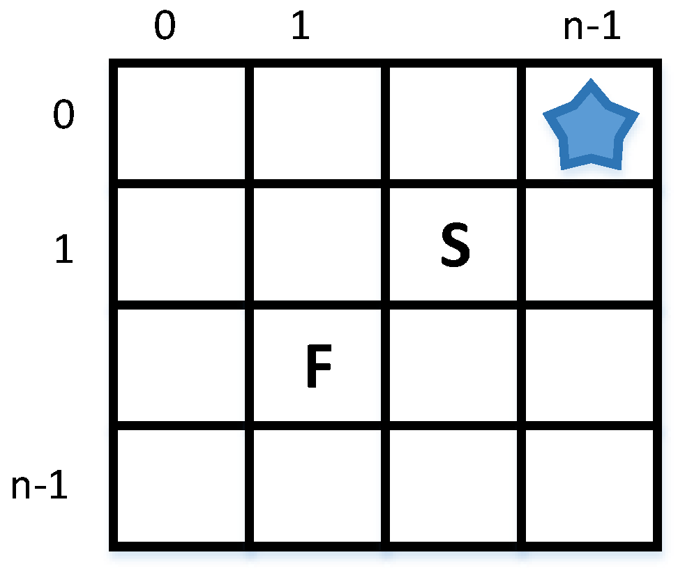
In this section, we focus on the shepherding problem introduced in Section 1. We first consider the one-dimensional version of the problem where both farmer and the sheep move in a line. Thus, we have a row of n cells that the sheep/farmer can be in. Thus, we have two variables c f and c s which represent the location of the farmer and the sheep, respectively (see Figure 5). The farmer and the sheep can change their location at most by one cell at a time.
The rightmost cell is marked as the desired location. The farmer wants to steer the sheep to this cell. Thus, the invariant for the problem is { s | c s ( s ) = n 1 } , where n is the number of cells in the row. The sheep always tries to increase its distance with the farmer. When the farmer and the sheep are in the same location, the sheep non-deterministically decides to go to the right or left, if it has space in its both left and right. When the sheep is in the desired location, it stops moving further. With this explanation, the set of environment transitions is
δ e = { ( s 0 , s 1 ) | c s ( s 0 ) n 1 c f ( s 0 ) = c f ( s 1 ) ( c f ( s 0 ) < c s ( s 0 ) c s ( s 0 ) < n 1 c s ( s 1 ) = c s ( s 0 ) + 1 c f ( s 0 ) > c s ( s 0 ) c s ( s 0 ) > 0 c s ( s 1 ) = c s ( s 0 ) 1 c f ( s 0 ) = c s ( s 0 ) c s ( s 0 ) < n 1 c s ( s 1 ) = c s ( s 0 ) + 1 c f ( s 0 ) = c s ( s 0 ) c s ( s 0 ) > 0 c s ( s 1 ) = c s ( s 0 ) 1 ) }
Also, since the farmer cannot move more than one cell in one step, the set of program restrictions is
δ r = { ( s 0 , s 1 ) | | c f ( s 0 ) c f ( s 1 ) | > 1 } .
Because of the non-determinism in the movement of the sheep, a program for the farmer can go into an infinite loop such that it never reaches the goal state. To understand how that can happen, consider this scenario: suppose both farmer and sheep are in the cell 0. Since the left side of the sheep is closed, it can only move to the right. Thus, it moves to the second cell. Now, suppose the farmer also decides to go to the second cell. Thus, again both of them are in the same cell. However, this time, since the left side of the sheep is open, it may decide to go there. Suppose sheep decides to go the left cell. Then, the farmer also goes back to the first cell. Once again, they are both in the first cell and the same scenario can repeat forever. A correct program for the farmer utilizes the behavior of the sheep, while avoiding going into an infinite loop and steers the sheep to the desired location.
We modeled this problem using JavaRepair for different sizes. We used a program with an empty set of transitions as the input program. Algorithm 1 successfully adds stabilization to the given program. Table 1 shows the repair time for different sizes.

6.1.2. Two-Dimensional Stabilizing Shepherding Problem

In this section, we consider the shepherding problem described in Section 6.1.1 in a two-dimensional space. Thus, instead of a single row of cells, we have a grid of cells where the sheep and the farmer can move. Thus, we have four variables r f , c f , r s and c s that represent the row and column of the farmer and the sheep, respectively (see Figure 6).
The upper right corner of the grid is the desired location. Thus, the invariant for this problem is { s | r s ( s ) = 0 c s ( s ) = n 1 } , where again n is the number of cells in a row. The sheep again tries to increases its distance with the farmer. The sheep and the farmer can only change either their row or column by at most one at each step. As in Section 6.1.1, sheep stops moving once it is in the desired location. With this explanation, the set of environment transitions is
δ e = { ( s 0 , s 1 ) | ¬ ( r s ( s 0 ) = 0 c s ( s 0 ) = n 1 ) ( r f ( s 0 ) = r f ( s 1 ) c f ( s 0 ) = c f ( s 1 ) ) ( c s ( s 0 ) = c s ( s 1 ) r s ( s 0 ) = r s ( s 1 ) ) ( c f ( s 0 ) < c s ( s 0 ) c s ( s 0 ) < n 1 c s ( s 1 ) = c s ( s 0 ) + 1 c f ( s 0 ) > c s ( s 0 ) c s ( s 0 ) > 0 c s ( s 1 ) = c s ( s 0 ) 1 c f ( s 0 ) = c s ( s 0 ) c s ( s 0 ) < n 1 c s ( s 1 ) = c s ( s 0 ) + 1 c f ( s 0 ) = c s ( s 0 ) c s ( s 0 ) > 0 c s ( s 1 ) = c s ( s 0 ) 1 r f ( s 0 ) < r s ( s 0 ) r s ( s 0 ) < n 1 r s ( s 1 ) = r s ( s 0 ) + 1 r f ( s 0 ) > r s ( s 0 ) r s ( s 0 ) > 0 r s ( s 1 ) = r s ( s 0 ) 1 r f ( s 0 ) = r s ( s 0 ) r s ( s 0 ) < n 1 r s ( s 1 ) = r s ( s 0 ) + 1 r f ( s 0 ) = r s ( s 0 ) r s ( s 0 ) > 0 r s ( s 1 ) = r s ( s 0 ) 1 ) }
Also, the set of program restrictions is
δ r = { ( s 0 , s 1 ) | | c f ( s 0 ) c f ( s 1 ) | + | r f ( s 0 ) r f ( s 1 ) | > 1 } .
Like one-dimensional case discussed in Section 6.1.1, with a poorly designed farmer, here is also possible to chase the sheep forever and never reach the desired state. Table 1 shows the repair time using JavaRepair for this problem for different sizes.

6.2. Addition of Fault-Tolerance

In this section, we use the JavaRepair package to repair/synthesis fault-tolerant programs for two other variations of the shepherding problem. We first create a failsafe fault-tolerant program in Section 6.2.1. Next, we create a masking fault-tolerant program in Section 6.2.2.

6.2.1. Failsafe Fault-Tolerant Shepherding Problem

For this variation, we change the two-dimensional version described in Section 6.1.2 as follows: there is no requirement of steering the sheep to the desired location. Instead, we require that the farmer must be always close to the sheep. Specifically, we require that the farmer and sheep can be far apart at most by one row or one cell. We model this requirement as a safety property with the set of bad transitions
δ b = { ( s 0 , s 1 ) | ¬ ( r s ( s 1 ) = r f ( s 1 ) c s ( s 1 ) = c f ( s 1 ) | r s ( s 1 ) r f ( s 1 ) | = 1 c s ( s 1 ) = c f ( s 1 ) r s ( s 1 ) = r f ( s 1 ) | c s ( s 1 ) c f ( s 1 ) | = 1 ) } .
The invariant, the set of environment transitions δ e and the set of program restrictions δ r are the same as those for two-dimensional case explained in Section 6.1.2. For addition of fault-tolerance we have a set of faults as the input. We consider two sets of faults and try to repair the program with each of them. The first set captures faults that can change the state of the program arbitrary, that is, for any state the program may change to any other state. We denote this set by f a r b i t r a r y . The second set of fault transitions that we consider captures faults that cause the system transition to a state where both farmer and sheep co-locate in one of the cells except the desired cell. We model this transition as a set of fault transitions
f s a m e l o c a t i o n = { ( s 0 , s 1 ) | r s ( s 0 ) = 0 c s ( s 0 ) = n 1 r s ( s 1 ) = r f ( s 1 ) c s ( s 1 ) = c f ( s 1 ) ¬ ( r s ( s 1 ) = 0 c s ( s 1 ) = n 1 ) }
We modeled this problem using JavaRepair for different sizes. The Algorithm 2 does not find any solution for the case of arbitrary faults, f a r b i t r a r y . From the completeness of Algorithm 2, we know that there is no solution for this case. On the other hand, the algorithm finds a solution for f s a m e - l o c a t i o n . Table 2 shows the repair time for different sizes.

6.2.2. Masking Fault-Tolerant Shepherding Problem

In this section, we add the requirement of steering the sheep to the desired location to the failsafe version explained in Section 6.2.1. Note that this requirement is weaker than the one specified in the stabilization version explained in Section 6.1.2 where we required that the farmer must steer the sheep to the desired location starting from any arbitrary state. On the other hand, in this section, we require that the farmer should steer the sheep to the goal state once the program starts in states reached by the fault transitions (i.e., fault-span). The invariant, the set of environment transitions and the set of program restrictions are the same as those defined in Section 6.2.1. Like Section 6.2.1, we consider two sets of fault transitions f a r b i t r a r y and f s a m e - l o c a t i o n . Like failsafe case, there is no solution for arbitrary faults but for same-location faults, Algorithm 3 finds a solution. Table 2 shows the addition time for this problem.

7. Discussion and Extensions of Algorithms

In this section, we consider problems related to those addressed in Section 3 and Section 5. Our first variation focuses on Definition 6. In this definition, we assumed that the environment is fair. Specifically, at least k 1 actions execute between any two environment actions. We consider variations where (1) this property is satisfied eventually. In other words, for some initial computation, environment actions may prevent the program from executing. However, eventually, fairness is provided to program actions and (2) program actions are given even with reduced fairness. Specifically, we consider the case where several environment actions can execute in a row but program actions execute infinitely often.
Our second variation is related to the invariant of the revised program, S and the invariant of the original program, S. In the case of adding stabilization, we considered S = S whereas, in the case of adding fault-tolerance, we considered S S .
Changes for adding stabilization and fault-tolerance with an eventually fair environment. No changes are required to Algorithm 1 even if the environment is eventually fair. This is due to the fact that this algorithm constructs programs that provide recovery from any state, that is, it will provide recovery from the state reached after the point when fairness is restored. For Algorithm 2 and Algorithm 3, we should change the input f to include δ e δ f . The resulting algorithm will ensure that the generated program will allow unfair execution of the program in initial states. However, fault-tolerance will be provided when the fairness is restored.
Changes for adding stabilization and fault-tolerance with multiple consecutive environment actions. If environment actions can execute consecutively, we can change input δ e to be its transitive closure. In other words, if ( s 0 , s 1 ) and ( s 1 , s 2 ) are transitions in δ e , we add ( s 0 , s 2 ) to δ e . With this change, the constructed program will provide stabilization or fault-tolerance even if environment transitions can execute consecutively.
Changes for adding stabilization and fault-tolerance based on relation between S (invariant of the fault-tolerant program) and S (invariant of the fault-intolerant program). No changes are required to Algorithm 1 even if we change the problem statement to allow S S without affecting soundness or completeness. Regarding soundness, observe that the program generated by this algorithm ensures S = S . Hence, it trivially satisfies S S . Regarding completeness, the intuition is that if it was impossible to recover to states in S then it is impossible to recover to states that are a subset of S. Regarding Algorithm 2 and Algorithm 3, if S is required to be equal to S then they need to be modified as follows: in these algorithms if any state S is removed (due to it being in m s 2 , deadlocks, etc.) then they should declare failure.
Other applications of our algorithms. In this paper, we considered the shepherding application as a way to illustrate the role of environment actions. The shepherding program is an instance of several other programs. For example, consider a smart cruise controller. In this example, we have two cars, A and B where car A is the car in front and car B is trying to match the speed of car A and maintain a safe distance. Now, considering from the perspective of car B, actions of car A are environment actions that are unchangeable. These actions are essential (without these actions, car B will not be able to satisfy its objectives) and disruptive. In other words, car A plays the same role as the sheep and car B plays the same role as the farmer.
It is also applicable in an example such as merging on a highway. In this example (when viewed from the perspective of the car that is merging), actions of other cars are the same as the role played by sheep in the shepherding problem. More generally, if we have a system with multiple components/processes where only some components are changeable, then these components would be modeled as farmer actions whereas unchangeable actions play the role of the sheep.

8. Related Work

This paper focuses on the addition of fault-tolerance properties in the presence of unchangeable environment actions. This problem is an instance of model repair where some existing model/program is repaired to add new properties such as safety, liveness, fault-tolerance and so forth. Model repair with respect to CTL properties was first considered in [11] and abstraction techniques for the same are presented in [12]. Previously, Bonakdarpour et al. [13] has considered the problem of model repair for UNITY specifications [14]. These results identify complexity results for adding properties such as invariant properties, leads-to properties and so forth. Repair of probabilistic algorithms has also been considered in the literature [15]. Roohitavaf and Kulkarni [16] provide repair algorithms for cases where the new desired properties are in conflict with existing properties.
The problem of adding fault-tolerance to an existing program has been discussed in the absence of environment actions. This work includes work on controller synthesis [17,18,19,20]. A tool for automated addition of fault-tolerance to distributed programs is presented in [1]. This work utilizes BDD based techniques to enable the synthesis of programs with state space exceeding 10 100 . However, this work does not include the notion of environment actions that cannot be removed. Hence, applying it in contexts where some processes/components cannot be changed will result in unacceptable solutions. Model repair for distributed programs using a two-phase lazy approach is proposed in [21].
The work on game theory [22,23,24] has focused on the problem of repair with the 2-player game where the actions of the second player are not changed. However, this work does not address the issue of fault-tolerance. Also, the role of the environment in our work is more general than that in [22,23,24]. Specifically, in the work on game theory, it is assumed that the players play in an alternating manner. By contrast, we consider more general interaction with the environment. In [25], authors have presented an algorithm for adding recovery to component-based models. They consider the problem where we cannot add to the interface of a physical component. However, it does not consider the issue of unchangeable actions considered in our work.
Hajisheykhi et al. [26,27] focus on the notion of auditable events which captures special events for which the program must first transition to a special state called auditable state where every process is aware of the auditable events, before returning to the normal states. Thus, compared with fault-span considered in this paper (cf. Definition 14), the set of states that a program may reach other than its states includes states that can be reached by fault transitions and those that can be reached by auditable transitions. Considering the problem of auditable restoration in presence of environment actions is an interesting future work.

9. Conclusions

In this paper, we focused on the problem of adding fault-tolerance to an existing program which consists of some actions that are unchangeable. These unchangeable actions arise due to interaction with the environment, inability to change parts of the existing program, constraints on physical components in a cyber-physical system and so on. We presented algorithms for adding stabilization and fault-tolerance. These algorithms are sound and complete and run in polynomial time (in the state space).
We considered the cases where (1) all fault-free behaviors are preserved in the fault-tolerant program, or (2) only a nonempty subset of fault-free behaviors are preserved in the fault-tolerant program. We also considered the cases where (1) environment actions can execute with any frequency for an initial duration and (2) environment actions can execute more frequently than programs. In all these cases, we demonstrated that our algorithm can be extended while preserving soundness and completeness. We provided a Java package including the implementation of our algorithm using BDDs. We presented some of our experimental results of adding stabilization and fault-tolerance using JavaRepair.
There are several future extensions to this work. One of the extensions has to deal with partial observability in distributed or embedded systems. Algorithms in this paper need to be revised by taking into account scenarios where, due to partial observability, one transition added or removed corresponds to a group of transitions [28]. Another extension is to extend the JavaRepair package so that it can be used efficiently and with a reduced learning curve. Yet another extension is to deal with the issue of time in embedded and cyber-physical systems. Specifically, in a CPS, we expect physical components to execute at a certain speed. In other words, an action of the physical component can be thought of to take some time between ϵ 1 and ϵ 2 . In turn, this affects the number of steps a computational component can execute in the middle. Note that this maps to the value of k used in our algorithms. Also, our definition of computation requires that the environment cannot execute too frequently. We also intend to extend to cases where a similar restriction also applies to computational components.

Author Contributions

Supervision, S.K.; Writing—original draft, M.R.

Funding

This work is supported in part by NSF CPS 1329807, NSF SaTC 1318678, and NSF XPS 1533802.

Conflicts of Interest

The authors declare no conflict of interest.

Abbreviations

The following abbreviations are used in this manuscript:
MDPIMultidisciplinary Digital Publishing Institute
DOAJDirectory of open access journals
TLAThree letter acronym
LDlinear dichroism

Appendix A. Soundness, Completeness and Complexity of Algorithm 2

Appendix A.1. Soundness

The following lemma splits condition C1 into easily verifiable conditions that assist in proving the soundness of Algorithm 2.
Lemma A1.
The conditionC1in the problem definition of addition of fault-tolerance is satisfied for k = 2 if conditions below are satisfied:
1. 
S S
2. 
δ p | S δ p | S
3. 
s 1 : s 0 , s 2 , s 3 : s 0 S ( s 0 , s 1 ) , ( s 1 , s 2 ) δ e ( s 1 , s 3 ) δ p : s 4 : : ( s 1 , s 4 ) δ p
4. 
s 0 : : ( s 1 : : ( s 0 , s 1 ) δ p δ e )
Proof. 
We show by induction that if all conditions of the lemma are satisfied, then every prefix of any p [ ] 2 δ e computation that starts from a state in S is a prefix of a p [ ] 2 δ e computation which starts in S.
Base case: Let s 0 be the prefix of a p [ ] 2 δ e computation that starts from S . Since S S , s 0 S . Thus, s 0 is also a prefix of a p [ ] 2 δ e computation that starts from S.
Induction hypothesis: The theorem holds for s 0 , s 1 , , s i .
Induction step: We show theorem holds for s 0 , s 1 , , s i + 1 . Since p δ e is closed in S , we know that s i + 1 S . We have two cases for ( s i , s i + 1 ) :
Case 1 ( s i , s i + 1 ) δ p
From δ p | S δ p | S , we have ( s i , s i + 1 ) δ p . Therefore, if s 0 , s 1 , , s i is a prefix of p [ ] 2 δ e , then s 0 , s 1 , , s i , s i + 1 is a prefix of p [ ] 2 δ e .
Case 2 ( s i , s i + 1 ) δ e :
Two sub-cases are possible below this case:
Case 2.1 ( s i 1 , s i ) δ p
In this case, as we have reached s i by a program transition, even with the fairness assumption, ( s i , s i + 1 ) can occur in p [ ] 2 δ e , Therefore, if s 0 , s 1 , , s i is a prefix of p [ ] 2 δ e , then s 0 , s 1 , , s i , s i + 1 is a prefix of p [ ] 2 δ e .
Case 2.2 ( s i 1 , s i ) δ e
In this case, there does not exist s such that ( s i , s ) δ p (otherwise, because of fairness ( s i , s i + 1 ) cannot be in any prefix of p [ ] 2 δ e ). Now, according to condition 3, we know there does not exist state s such that ( s i , s ) δ p . Thus, even with the fairness assumption ( s i , s i + 1 ) can occur in p [ ] 2 δ e . Therefore, if s 0 , s 1 , , s i is a prefix of p [ ] 2 δ e , then s 0 , s 1 , , s i , s i + 1 is a prefix of p [ ] 2 δ e .
Since every prefix of p [ ] 2 δ e that starts from a state in S is a prefix of p [ ] 2 δ e which starts in S, C1 is satisfied. □
Theorem A1.
Algorithm 2 is sound.
Proof. 
To show the soundness of our algorithm, we need to show that the three conditions of the addition problem are satisfied.
C1: Consider a computation c of p [ ] 2 δ e that starts from a state in S . By construction, c starts from a state in S and δ p | S is a subset of δ p | S . Therefore, the first two requirements of Lemma A1 are satisfied. Regarding the third requirement of Lemma A1, suppose that there exists s 1 in S such that s 0 , s 2 , s 3 : s 0 S ( s 0 , s 1 ) , ( s 1 , s 2 ) δ e ( s 1 , s 3 ) δ p but s 4 : : ( s 1 , s 4 ) δ p . From s 2 , s 3 : : ( s 1 , s 2 ) δ e ( s 1 , s 3 ) δ p and s 4 : : ( s 1 , s 4 ) δ p we can conclude that s 1 is in m s 3 . Then, from ( s 0 , s 1 ) δ e , we know that s 0 is in m s 4 , which is contradiction as s 0 is in S. Finally, the fourth condition is satisfied by the fact that S does not include any deadlock state. Since all conditions of Lemma A1 are satisfied, condition C1 holds.
C2: We need to show that p is a failsafe fault-tolerant revision for p. Thus, we need to show constraints of Definition 15 are satisfied.
From C1, S S , the assumption that p [ ] 2 δ e satisfies s p e c from S, S and S is closed in p δ e , all constrains of Definition 10 are satisfied. Thus, p [ ] 2 δ e 2-satisfies s p e c from S .
Let s p e c be S f , L v . Consider prefix c of p [ ] 2 δ e [ ] f such that c starts from a state in S . If c does not satisfy S f then there exists a prefix of c, say s 0 , s 1 , , s n , such that it has a transition in δ b . W.l.o.g., let s 0 , s 1 , , s n be the smallest such prefix. It follows that ( s n 1 , s n ) δ b , hence, ( s n 1 , s n ) m t . By construction, p does not contain any transition in m t . Thus, ( s n 1 , s n ) is a transition of f or δ e . If it is in f then s n 1 m s 1 (i.e., s n 1 m s 2 ). If it is in δ e then s n 1 m s 2 . Therefore, in both cases, s n 1 m s 2 and ( s n 2 , s n 1 ) m t . Again, by construction, we know that δ p does not contain any transition in m t , so ( s n 2 , s n 1 ) is either in f or δ e . If it is in f then s n 2 m s 1 (i.e., s n 2 m s 2 ). If it is in δ e two cases are possible:
(1) ( s n 1 , s n ) f . In this case, as stated before, s n 1 m s 1 , so s n 2 m s 2 .
(2) ( s n 1 , s n ) δ e . Since ( s n 1 , s n ) δ e δ b , from the fact the original program satisfies s p e c from S, we conclude that s n 1 S (i.e., s n 1 S ). In this case, all transitions starting from s n 1 should be in m t . If this is not the case then this implies that there exists a state s such that ( s n 1 , s ) is not in m t and we would have added it to δ p by Line 22, as S n 1 is outside S . Since all transitions from s n 1 are in m t , s n 1 is in m s 1 (by Line 7). Hence, s n 2 is in m s 2 . Continuing this argument further leads to the conclusion that s 0 m s 2 . This is a contradiction, as we know S does not include any state in m s 2 . Thus, any prefix of p [ ] 2 δ e [ ] f satisfies S f . Thus, C2 holds.
C3: Any ( s 0 , s 1 ) δ r , is in m t . By construction, δ p does not have any transition in m t . Hence, C3 holds. □

Appendix A.2. Completeness

Now, we focus on showing that Algorithm 2 is complete, that is, if there is a solution that satisfies the problem statement for adding failsafe fault-tolerance, Algorithm 2 finds one. The proof of completeness is based on the analysis of states that were removed from S. First, we note the following observation:
Observation 4.
For every state s 0 in m s 2 one of three cases below is true:
1. 
s 0 m s 1
2. 
s 1 : : ( s 0 , s 1 ) δ e s 1 m s 1
3. 
s 1 : : ( s 0 , s 1 ) δ e δ b
Now, for the rest of our discussion in this section, we assume that Algorithm 2 has declared failure for finding a failsafe fault-tolerant revision of program p = S p , δ p with invariant S. Let p = S p , δ p with invariant S be any revision for program p. Also, let f and δ e be a set of fault transitions and a set of environment transitions for p (i.e., p ), respectively. If there exists a computation prefix that reaches a state in m s 2 , there exists a computation with that prefix that either reaches a state in m s 1 , or executes a transition in δ b (i.e., violates safety). Specifically, we have the following lemma.
Lemma A2.
If α is a prefix of a p [ ] 2 δ e [ ] f computation and α = s i , , s m such that s i m s 2 , or α = s 0 , s i 1 , s i such that s i m s 2 and ( s i 1 , s i ) f δ p , then, there exists a suffix β such that α β is a p [ ] 2 δ e [ ] f computation and
  • j : j i : ( ( s j 1 , s j ) δ b ) , or
  • j : j i : ( s j m s 1 ) .
Proof. 
From Observation 4, we know there are three cases for s i . The first case is s i m s 1 . The theorem trivially holds for this case. In the second and the third case, there is an environment transition that either is a bad transition, or reaches a state in m s 1 . This transition can occur even with the fairness assumption, as the computation has started in s j , or we have reached s j with a fault or program transition. □
For states in m s 1 we have the following lemma that says in any given revision p for p, if there exists a computation prefix that reaches a state in m s 1 , then there exists a computation with that prefix that executes a transition in δ b .
Lemma A3.
If α = s 0 , , s i 1 , s i where s i m s 1 is a prefix of a p [ ] 2 δ e [ ] f computation, then, there exists a suffix β = s i + 1 , s i + 2 , such that α β is a p [ ] 2 δ e [ ] f computation and j : j i : ( s j , s j + 1 ) δ b .
Proof. 
We prove this inductively as we expand m s 1 :
Base case: m s 1 = { s 0 | s 1 : : ( s 0 , s 1 ) f δ b }
Let β be any p [ ] 2 δ e [ ] f computation starting from s 1 . Since fault transitions can execute in any state, α β is a p [ ] 2 δ e [ ] f computation such that ( s 0 , s 1 ) δ b .
Induction hypothesis: Theorem holds for current m s 1 .
Induction step: We show when we add a state to m s 1 , the theorem still holds for m s 1 . A state s 0 is added into m s 1 in three cases:
Case 1 s 1 : s 1 m s 2 : ( s 0 , s 1 ) f
In this case according to Lemma A2, a transition in δ b may occur, or a state in m s 1 can be reached. Hence, according to the induction hypothesis, a transition in δ b can occur in both cases.
Case 2 s 1 : : ( s 1 m s 1 ( s 0 , s 1 ) δ e ) ( s 2 : : ( s 0 , s 2 ) m t )
In this case, if according to fairness, ( s 0 , s 1 ) can occur, state s 1 m s 1 can be reached by ( s 0 , s 1 ) and according to the induction hypothesis, the theorem is proved. However, if ( s 0 , s 1 ) cannot occur, some other transition in δ p f should occur but we know such transition is in m t and reaches a state in m s 2 . Thus, according to Lemma A2, either a transition in δ b can occur, or a state in m s 1 can be reached. Hence, according to the induction hypothesis, a transition in δ b can occur in both cases.
Case 3 s 1 : : ( ( s 0 , s 1 ) δ e δ b ) ( s 2 : : ( s 0 , s 2 ) m t )
In this case, if, according to fairness, ( s 0 , s 1 ) can occur, by its occurrence a transition in δ b has occurred. However, if ( s 0 , s 1 ) cannot occur, some other transition in δ p f should occur but we know such a transition is in m t and reaches a state in m s 2 . Thus, according to Lemma A2, either a transition in δ b can occur or a state in m s 1 can be reached. Hence, according to the induction hypothesis, a transition in δ b can occur in both cases. □
The last lemma that we use to prove the completeness of Algorithm 2 is Lemma A4. This lemma states that having any state in m s 4 in the invariant of any give revision p of program p results in having new computation in the invariant that was not in the original program.
Lemma A4.
Let p = S p , δ p with invariant S be any revision for program p = S p , δ p with invariant S such that, S S and δ p | S δ p | S for S and δ p at the beginning of the loop on Lines 13–21. If S includes any state in m s 4 in any iteration of the loop on Lines 13–21, then there is a p [ ] 2 δ e computation that starts from S that is not a p [ ] 2 δ e .
Proof. 
Suppose there exists state s 0 S m s 4 . Then, there is a state, s m s 3 such that ( s 0 , s ) δ e and s 1 , s 2 : : ( s , s 1 ) δ e ( s , s 2 ) δ p s 3 : : ( s , s 3 ) δ p . Since δ p | S δ p | S , ( s 3 : : ( s , s 3 ) δ p ) . Since S is closed in p δ e , s and s 1 are in S , as well. Now, observe that s 0 , s , s 1 , is p [ ] 2 δ e computation but it is not a p [ ] 2 δ e computation, as because of fairness, ( s , s 1 ) δ e cannot occur when there exists ( s , s 2 ) δ p . □
Theorem A2.
Algorithm 2 is complete.
Proof. 
Suppose program p with invariant S solves the addition problem. We show that at any point of Algorithm 2, S must always be a subset of S . We prove this by looking at lines where we set S . According to Lemma A2 and Lemma A3, S cannot have any transition in m s 2 , because by starting from a state in m s 2 , a computation may execute a bad transition. In addition, S must be closed in δ p and cannot have any deadlock state. Thus, S S for S of Line 12. According to Lemma A4, S cannot include any state in m s 4 , because otherwise there is a p [ ] 2 δ e computation that is not p [ ] 2 δ e (contradiction to C1). Thus, S S for S of Line 20. Thus, always we have S S . Our algorithm declares failure only when S = . Thus, if our algorithm does not find any solution, from S S , we have S = (contradiction to Definition 11). □
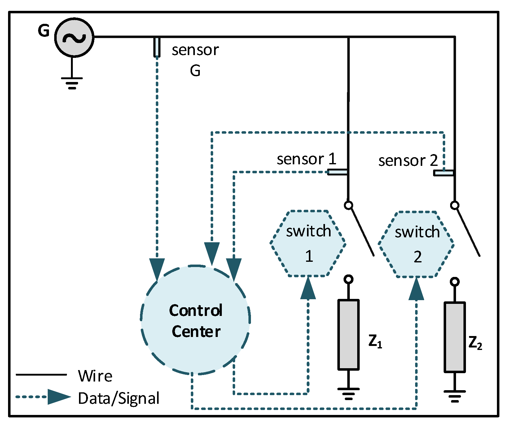
Appendix A.3. Time Complexity

Theorem A3.
Algorithm 2 is polynomial (in the state space of p)
Proof. 
The proof follows from the fact that each statement in Algorithm 2 is executed in polynomial time and the number of iterations is also polynomial. □

Appendix B. Soundness, Completeness, and Complexity of Algorithm uid141

Appendix B.1. Soundness

First, we show that the program constructed by Algorithm 3 never reaches a state in m s 1 . Specifically,
Lemma A5.
For any p [ ] 2 δ e [ ] f computation s 0 , s 1 , where s 0 S , there dose not exist s i such that s i is in m s 1 .
Proof. 
Consider a computation s 0 , s 1 , of p [ ] 2 δ e [ ] f where s 0 S . We proof by induction that for all i 0 , s i m s 1 :
Base case: i { 0 , 1 }
It is clear s 0 m s 1 , because m s 1 m s 2 and s 0 S and by construction, we know S m s 1 = (see Line 33). Also, s 1 m s 1 , because otherwise s 0 m s 2 that is contradiction to S m s 2 = .
Induction hypothesis: i : 0 i n : s i m s 1
Induction step: s n + 1 m s 1
Suppose s n + 1 m s 1 . Then, ( s n , s n + 1 ) m t . By construction, the program does not have any transition in m t . Thus, we have two cases for ( s n , s n + 1 ) :
Case 1: ( s n , s n + 1 ) f
In this case, s n m s 1 (by Line 28) that is contradictory to the induction hypothesis.
Case 2: ( s n , s n + 1 ) δ e
In this case, s n m s 2 . If n = 0 , then s 0 m s 2 that is contradiction to S m s 2 = . If n > 0 , then ( s n 1 , s n ) m t . By construction, the program does not have any transition in m t . Thus, we have two cases for ( s n 1 , s n )
Case 2.1: ( s n 1 , s n ) f :
In this case, s n 1 m s 1 that is contradictory to the induction hypothesis.
Case 2.2: ( s n 1 , s n ) δ e :
In this case, as both ( s n 1 , s n ) and ( s n , s n + 1 ) are in δ e , according to the fairness assumption, there does not exist a transition δ p starting from s n and it means that s n is added to m s 1 by Line 28 which is in contradiction with the induction hypothesis. □
Since we never reach any state in m s 1 starting from S and since any state in ¬ ( R R p ) is in m s 1 by Line 23, we conclude we never reach ¬ ( R R p ) . Thus, we have the following corollary:
Corollary A1.
R R p in the last iteration of loop on Lines 6–43 is a f-span for the program resulted by Algorithm 3.
The following lemma states that in every computation of the repaired program that starts from its invariant (i.e., S ), if the program reaches a state in R, in the rest of the computation it will reach S . Specifically,
Lemma A6.
For every δ p [ ] 2 δ e [ ] f computation s 0 , s 1 , such that s 0 S , for S and R in the last iteration of the loop on Lines 6–43, we have:
s i : s i R : ( j : j i : s j S ) .
Proof. 
We prove this lemma by induction as we expand set R:
Base case: R = S
The proof is trivial.
Induction hypothesis: Theorem holds for current R.
Induction step:
For any state s 0 that is added to R we have
s 2 : s 2 ( ¬ ( R R p ) m s 1 ) : ( s 0 , s 2 ) δ e ( s 1 : s 1 ( R R p ) m s 1 : ( s 0 , s 1 ) δ e ) ( s 2 : : ( s 0 , s 2 ) ( δ e δ b ) ) s 0 R p )
Thus, any environment transition either reaches R or R p . In the second case, since we have reached a state in R p by an environment transition, and since from any state in R p there is a program transition to R (cf. Line 17), based on the fairness assumption, the computation will reach R. Thus, in either case, we reach R. Since in the last iteration of loop on Lines 6–43, we do not change the set of transitions for states in R of the previous iteration, based on the induction hypothesis, the lemma is proved. □
The following lemma states that when the repaired program starts at its invariant S , if it reaches a state in R p R , in the rest of the its computation it will reach a state in S . Specifically,
Lemma A7.
For every δ p [ ] 2 δ e [ ] f computation s 0 , s 1 , such that s 0 S , for S , R p and R in the last iteration of loop on Lines 6–43, we have:
s i : s i R p R : ( j : j i : s j S ) .
Proof. 
Let s i ( R p R ) . Any state that is not in R is in m s 2 . Thus, ( s i 1 , s i ) m t . By construction, the program does not have any transition in m t . Thus, ( s i 1 , s i ) f δ e . If ( s i 1 , s i ) f , then s i 1 m s 1 that is a contradiction to Lemma A5. Thus, ( s i 1 , s i ) δ e . Since we have reached s i by an environment transition and s i R p , the computation will reach R and according to Lemma A6, the computation will reach S . □
Based on Lemmas A6 and A7, we have the following corollary that guarantees recovery to the invariant from R R p .:
Corollary A2.
For every δ p [ ] 2 δ e [ ] f computation s 0 , s 1 , such that s 0 S , for S , R p and R in the last iteration of loop on Lines 6–43, we have:
s i : s i R R p : ( j : j i : s j S ) .
Theorem A4.
Algorithm 3 is sound.
Proof. 
In order to show the soundness of our algorithm, we need to show that the three conditions of the problem statement are satisfied.
C1: Satisfaction of C1 for Algorithm 3 is the same as that for Algorithm 2 stated in the proof of the Theorem A1.
C2: We need to show that p is a masking fault-tolerant revision for p. Thus, we need to show the constraints of Definition 16 are satisfied. From C1, S S , the assumption that p [ ] 2 δ e satisfies s p e c from S, S and S is closed in p δ e , all constraints of Definition 10 are satisfied. Thus, p [ ] 2 δ e 2-satisfies s p e c from S .
Let s p e c = S f , L v . Consider prefix c of p [ ] 2 δ e [ ] f such that c starts from a state in S . If c does not satisfy S f , there exists a prefix of c, say s 0 , s 1 , , s n , such that it has a transition in δ b . W.l.o.g., let s 0 , s 1 , , s n be the smallest such prefix. It follows that ( s n 1 , s n ) δ b . Hence, ( s n 1 , s n ) m t . By construction, p does not contain any transition in m t . Thus, ( s n 1 , s n ) is a transition of f or δ e . If it is in f then s n 1 m s 1 which is a contradiction to Lemma A5. If it is in δ e then s n 1 m s 2 and ( s n 2 , s n 1 ) m t . Again, by construction, we know that δ p does not contain any transition in m t , so ( s n 2 , s n 1 ) is either in f or δ e . If it is in f then s n 2 m s 1 (contradiction to Lemma A5). If it is in δ e , as both ( s n 2 , s n 1 ) and ( s n 1 , s n ) are in δ e , according to the fairness assumption, there does not exist a transition of δ p starting from s n 1 and it means that s n 1 m s 1 , which is again a contradiction to Lemma A5. Thus, each prefix of c does not have a transition in δ b . Therefore, any prefix of p [ ] 2 δ e [ ] f satisfies S f .
As p 2-satisfies s p e c from S in environment δ e , any prefix of p [ ] 2 δ e [ ] f 2-satisfies S f and according to Corollary A1 and Corollary A2, p is masking 2-f-tolerant to s p e c from S in environment δ e with fault-span R R p for R and R p in the last iteration of the loop on Lines 6–43.
C3: Any ( s 0 , s 1 ) δ r , is in m t . By construction, p does not have any transition in m t , so C3 holds. □

Appendix B.2. Completeness

Like the proof of the completeness of Algorithm 2, the proof of the completeness of Algorithm 3 is based on the analysis of states that are removed from S. For Algorithm 3, we focus on the iterations of the loop on Lines 6–43.
Similar to Observation 1, we have the following observation for Algorithm 3:
Observation 5.
In any given iteration i of loop on 6–43, let R, R p and m s 1 be R, R p and m s 1 at the end of iteration i. Then, for any s 0 such that s 0 R and s 1 : : ( s 0 , s 1 ) δ e , we have
( s 2 : s 2 ¬ ( R R p ) m s 1 : ( s 0 , s 2 ) δ e )
( s 2 : : ( s 0 , s 2 ) δ e δ b ) .
We also note the following observation:
Observation 6.
For any s 0 such that s 0 R , either s 0 ¬ ( R R p ) , or s 2 : s 2 ¬ ( R R p ) m s 1 : ( s 0 , s 2 ) δ e .
Lemmas A8, A9, A10 and A11, Corollary A3 and Theorem A5 provided in the following, hold for any given iteration i of loop on Lines 6–43 assuming Algorithm 3 has declared failure. For these results, let p = S p , δ p with invariant S be any revision for program p = S p , δ p with invariant S such that S S , δ p δ p and δ p m t = . Consider S , δ p and m t at the beginning of iteration i and m s 1 , m s 2 , R and R p at the end of the iteration. Also, let f and δ e be a set of fault transitions and a set of environment transitions for p (i.e., p ), respectively.
The following lemma focuses on the situation where a given revision p reaches a state that our algorithm marks as ¬ ( R R p ) .
Lemma A8.
For every p [ ] 2 δ e [ ] f prefix α = s 0 , , s i such that s i ¬ ( R R p ) , there exists a suffix β such that α β is a p [ ] 2 δ e [ ] f computation and
  • ( s i , s i + 1 ) δ b , or
  • s i + 1 m s 1 , or
  • s i + 1 ¬ ( R R p ) , or
  • s i + 1 ( R p R ) s i + 2 ¬ ( R R p ) .
Proof. 
There are two cases for s i :
Case 1: s i is environment-enabled (see Definition 18) in prefix α = s 0 , s 1 , , s i :
According to Observation 5, there exists s ¬ ( R R p ) m s 1 such that ( s i , s ) δ e , ( s i , s ) δ e δ b . Any suffix that starts from s proves the theorem.
Case 2: s i is not environment-enabled in prefix α = s 0 , s 1 , , s i
The proof for this case is identical to the proof of Case 2 of Lemma 2. □
Corollary A3.
For every p [ ] 2 δ e [ ] f prefix α = s 0 , , s i such that s i ¬ ( R R p ) , there exists a suffix β such that α β is a p [ ] 2 δ e [ ] f computation and
  • j : j i : ( s j 1 , s j ) δ b , or
  • j : j i : s j m s 1 , or
  • i : i 0 : s i S .
The following lemma focuses on states that are marked as m s 2 .
Lemma A9.
If α is a prefix of a p [ ] 2 δ e [ ] f computation and α = s i , , s m such that s i m s 2 , or α = s 0 , s i 1 , s i such that s i m s 2 and ( s i 1 , s i ) f δ p , then, there exists a suffix β such that α β is a p [ ] 2 δ e [ ] f computation and
  • j : j i : ( ( s j 1 , s j ) δ b ) , or
  • j : j i : ( s j m s 1 ) , or
  • i : i 0 : s i S .
Proof. 
We prove this lemma by looking at lines where we expand m s 2 :
Line 4: m s 2 = m s 1 { s 0 | s 1 : ( s 0 , s 1 ) δ e δ b }
In this case, we add s 0 to m s 2 if either it is in m s 1 , or it has a ( s 0 , s 1 ) transition that is in δ b . If s 0 m s 1 , any computation starting from s 0 proves the theorem. Otherwise, any computation s 0 , s 1 , proves the theorem.
Line 24: m s 2 = m s 2 ¬ R :
According to Observation 6, there is a suffix (possibly ) that reaches ¬ ( R R p ) . According to Corollary A3 there is a computation that either reaches m s 1 , or never reaches S .
Line 29: m s 2 = m s 2 m s 1 { s 0 | s 1 : s 1 m s 1 : ( s 0 , s 1 ) δ e ) }
In this case, we add state s 0 to m s 2 , if s 0 is in m s 1 or can reach state s 1 m s 1 with an environment transition. If s 0 m s 1 , any computation starting from s 0 proves the theorem. Otherwise, any computation s 0 , s 1 , proves the theorem. Note that, since we have started the computation from s 0 , or we have reached s 0 with a fault or program transition, even with the fairness assumption, the environment transition ( s 0 , s 1 ) can execute. □
The following lemma states that reaching any state in m s 1 will result in bad consequences that can be either executing a bad transition or never recovering to the invariant. Specifically,
Lemma A10.
If α = s 0 , , s i 1 , s i where s i m s 1 is a prefix of a p [ ] 2 δ e [ ] f computation, then, there exists a suffix β = s i + 1 , s i + 2 , such that α β is a p [ ] 2 δ e [ ] f computation and
  • j : j i : ( s j , s j + 1 ) δ b , or
  • j : j 0 : s j S .
Proof. 
We prove this theorem inductively based on where we expand m s 1 :
Base Case: m s 1 = { s 0 | ( s 0 , s 1 ) f δ b }
Let β be any p [ ] 2 δ e [ ] f computation starting from s 1 . Since fault transitions can execute in any state, α β is a p [ ] 2 δ e [ ] f computation such that ( s 0 , s 1 ) δ b .
Induction hypothesis: Theorem holds for current m s 1 .
Induction step: We look at lines where we add a state to s 0 :
Line 23: m s 1 = m s 1 ¬ ( R R p )
According to Corollary A3, there is a suffix that either runs a transition in δ b , never reaches S , or reaches a state in m s 1 . Thus, the theorem is proved by the induction hypothesis.
Line 28: m s 1 = m s 1 { s 0 | s 1 : s 1 m s 2 : ( s 0 , s 1 ) f } { s 0 | s 1 : s 1 m s 1 : ( s 0 , s 1 ) δ e ) ( s 0 , s 1 ) ( δ e δ b ) s 2 : : ( s 0 , s 2 ) δ p }
We add state s 0 to m s 1 in three cases in this line:
Case 1 s 1 : s 1 m s 2 : ( s 0 , s 1 ) f
In this case according to Lemma A9, a transition in δ b may occur, or there is a suffix that never reach S , or a state in m s 1 can be reached. Thus, according to the induction hypothesis, the theorem is proved.
Case 2 s 1 : : ( s 1 m s 1 ( s 0 , s 1 ) δ e ) ( s 2 : : ( s 0 , s 2 ) δ p )
In this case, if according to fairness, ( s 0 , s 1 ) can occur, state s 1 m s 1 can be reached by ( s 0 , s 1 ) and according to the induction hypothesis, the theorem is proved. However, if ( s 0 , s 1 ) cannot occur, some other transition t δ p f occurs. Since s 1 : s 1 m s 1 : ( s 0 , s 1 ) δ e , we know that s 0 R . By construction, δ p contains any transition from states ¬ R to R. Since s 2 : : ( s 0 , s 2 ) δ p , we conclude t goes to a state in ¬ R (i.e., m s 2 ). Thus, according to Lemma A9 either a transition in δ b can occur, or there is a suffix that never reaches S , or a state in m s 1 can be reached. Thus, according to the induction hypothesis, the theorem is proved.
Case 3 s 1 : : ( ( s 0 , s 1 ) δ e δ b ) ( s 2 : : ( s 0 , s 2 ) δ p )
In this case, if according to fairness, ( s 0 , s 1 ) can occur, by its occurrence a transition in δ b has occurred. However, if ( s 0 , s 1 ) cannot occur, some other transition in δ p should occur. Since s 1 : : ( ( s 0 , s 1 ) δ e δ b ) , s 0 R . Our algorithm add any possible program transition that is not m t and goes to a state in R to s 0 in Line 17. Since there is no such transition, any transition in δ p either is in m t or goes to ¬ R . In either case, we have a computation that reaches a state in m s 2 starting from s 0 . Thus, according to Lemma A9, either a transition in δ b can occur, or there is suffix that never reaches S , or a state in m s 1 can be reached. Thus, according to the induction hypothesis, the theorem is proved. □
Like Lemma A4 for Algorithm 2, we have following lemma for m s 4 for Algorithm 3.
Lemma A11.
If S includes any state in m s 4 in any iteration of the loop on Lines 13–21, then there is a p [ ] 2 δ e computation that starts from S that is not a p [ ] 2 δ e .
Proof. 
The proof of this lemma is very similar to that of Lemma A4. □
Theorem A5.
Algorithm 3 is complete.
Proof. 
Suppose program p and invariant S solve transformation problem. We show that at any point of Algorithm 3, S must always be a subset of S . We prove this by looking at lines where we set S .
In the first iteration of the loop on Lines 6–43, S = S . According to constraint C1 of the problem definition in Section 5.1, S S . Thus, S S for the S at the beginning of the first iteration of the loop on Lines 6–43. According to Lemmas A9 and A10, S cannot have any transition in m s 2 in first iteration of the loop on Line 6–43, because by starting from a state in m s 2 , a computation may execute a bad transition, or reach a state outside S from which there is a computation that never reaches S (i.e., never reaches S ). In addition, S must be closed in δ p and cannot have any deadlock state. Thus, S S for S at Line 33.
According to Lemma A11, S cannot include any state in m s 4 in the first iteration of the loop of Lines 6–43, because otherwise there is a p [ ] 2 δ e computation that is not p [ ] 2 δ e (contradiction to C1). Thus, S S for S at the end of the first iteration of the loop on Lines 6–43.
With the induction, we conclude that S cannot include any states in m s 2 or m s 4 in next iterations of the loop of Lines 6–43. Thus, always we have S S . Our algorithm declares failure only when S = . Thus, if our algorithm does not find any solution, from S S , we have S = (contradiction to Definition 11). □

Appendix B.3. Time Complexity

Theorem A6.
Algorithm 3 is polynomial (in the state space of p)
Proof. 
t The proof follows from the fact that each statement in Algorithm 3 is executed in polynomial time and the number of iterations is also polynomial. □

References

  1. Bonakdarpour, B.; Kulkarni, S.S.; Abujarad, F. Symbolic Synthesis of Masking Fault-tolerant Programs. Springer J. Distrib. Comput. 2012, 25, 83–108. [Google Scholar] [CrossRef]
  2. Bonakdarpour, B.; Kulkarni, S.S. Active Stabilization. In Proceedings of the Stabilization, Safety, and Security of Distributed Systems, 13th International Symposium, SSS 2011, Grenoble, France, 10–12 October 2011; Volume 6976, pp. 77–91. [Google Scholar]
  3. Roohitavaf, M.; Kulkarni, S. Stabilization and Fault-tolerance in Presence of Unchangeable Environment Actions. In Proceedings of the 17th International Conference on Distributed Computing and Networking, Singapore, 4–7 January 2016; ACM: New York, NY, USA, 2016; pp. 19:1–19:10. [Google Scholar] [CrossRef]
  4. JavaRepair. Available online: https://github.com/roohitavaf/JavaRepair (accessed on 1 July 2019).
  5. Alpern, B.; Schneider, F.B. Defining liveness. Inf. Process. Lett. 1985, 21, 181–185. [Google Scholar] [CrossRef]
  6. Arora, A.; Gouda, M.G. Closure and Convergence: A Foundation of Fault-Tolerant Computing. IEEE Trans. Softw. Eng. 1993, 19, 1015–1027. [Google Scholar] [CrossRef]
  7. Dijkstra, E.W. Self-stabilizing Systems in Spite of Distributed Control. Commun. ACM 1974, 17, 643–644. [Google Scholar] [CrossRef]
  8. Dolev, S. Self-Stabilization; MIT Press: Cambridge, MA, USA, 2000. [Google Scholar]
  9. Kundur, D.; Feng, X.; Liu, S.; Zourntos, T.; Butler-Purry, K. Towards a Framework for Cyber Attack Impact Analysis of the Electric Smart Grid. In Proceedings of the First IEEE International Conference on Smart Grid Communications, Gaithersburg, MD, USA, 4–6 October 2010; pp. 244–249. [Google Scholar]
  10. Roohitavaf, M.; Kulkarni, S. Collaborative Stabilization. In Proceedings of the 2016 IEEE 35th Symposium on Reliable Distributed Systems (SRDS), Budapest, Hungary, 26–29 September 2016; pp. 259–268. [Google Scholar]
  11. Buccafurri, F.; Eiter, T.; Gottlob, G.; Leone, N. Enhancing Model Checking in Verification by AI Techniques. Artif. Intell. 1999, 112, 57–104. [Google Scholar] [CrossRef]
  12. Chatzieleftheriou, G.; Bonakdarpour, B.; Smolka, S.A.; Katsaros, P. Abstract Model Repair. In Proceedings of the NASA Formal Methods Symposium (NFM), Norfolk, VA, USA, 3–5 April 2012. [Google Scholar]
  13. Bonakdarpour, B.; Ebnenasir, A.; Kulkarni, S.S. Complexity Results in Revising UNITY Programs. ACM Trans. Auton. Adapt. Syst. (TAAS) 2009, 4, 5. [Google Scholar] [CrossRef]
  14. Chandy, K.M.; Misra, J. Parallel Program Design: A Foundation; Addison-Wesley Longman Publishing Co. Inc.: Boston, MA, USA, 1988. [Google Scholar]
  15. Samanta, R.; Deshmukh, J.V.; Emerson, E.A. Automatic Generation of Local Repairs for Boolean Programs. In Proceedings of the Formal Methods in Computer-Aided Design (FMCAD), Portland, OR, USA, 17–20 November 2008; pp. 1–10. [Google Scholar]
  16. Roohitavaf, M.; Kulkarni, S.S. Automatic Addition of Conflicting Properties. In Proceedings of the International Symposium on Stabilization, Safety, and Security of Distributed Systems, Lyon, France, 7–10 November 2016; pp. 310–326. [Google Scholar]
  17. Ramadge, P.J.; Wonham, W.M. The control of discrete event systems. Proc. IEEE 1989, 77, 81–98. [Google Scholar] [CrossRef]
  18. Girault, A.; Rutten, É. Automating the addition of fault tolerance with discrete controller synthesis. Form. Methods Syst. Des. (FMSD) 2009, 35, 190–225. [Google Scholar] [CrossRef] [Green Version]
  19. Cho, K.H.; Lim, J.T. Synthesis of Fault-Tolerant Supervisor for Automated Manufacturing Systems: A Case Study on Photolithography Process. IEEE Trans. Robot. Autom. 1998, 14, 348–351. [Google Scholar]
  20. Chen, J.; Roohitavaf, M.; Kulkarni, S.S. Ensuring Average Recovery with Adversarial Scheduler. In Proceedings of the LIPIcs-Leibniz International Proceedings in Informatics, Rennes, France, 14–17 December 2015. [Google Scholar]
  21. Roohitavaf, M.; Lin, Y.; Kulkarni, S.S. Lazy repair for addition of fault-tolerance to distributed programs. In Proceedings of the 2016 IEEE International Parallel and Distributed Processing Symposium, Chicago, IL, USA, 23–27 May 2016; pp. 1071–1080. [Google Scholar]
  22. Pnueli, A.; Rosner, R. On the synthesis of a reactive module. In Proceedings of the Principles of Programming Languages (POPL), Austin, Texas, USA, 11–13 January 1989; pp. 179–190. [Google Scholar]
  23. Pnueli, A.; Rosner, R. On The Synthesis of An Asynchronous Reactive Module. In International Colloquium on Automata, Languages, and Programming; Springer: Berlin/Heidelberg, Germany, 1989; pp. 652–671. [Google Scholar]
  24. Jobstmann, B.; Griesmayer, A.; Bloem, R. Program Repair as a Game. In Proceedings of the Conference on Computer Aided Verification (CAV), Scotland, UK, 6–10 July 2005; pp. 226–238. [Google Scholar]
  25. Bonakdarpour, B.; Lin, Y.; Kulkarni, S.S. Automated Addition of Fault Recovery to Cyber-physical Component-based Models. In Proceedings of the ACM International Conference on Embedded Software (EMSOFT), New York, NY, USA, 9–14 October 2011; pp. 127–136. [Google Scholar]
  26. Hajisheykhi, R.; Roohitavaf, M.; Kulkarni, S.S. Auditable restoration of distributed programs. In Proceedings of the 2015 IEEE 34th Symposium on Reliable Distributed Systems (SRDS), Montreal, QC, Canada, 28 September–1 October 2015; pp. 37–46. [Google Scholar]
  27. Hajisheykhi, R.; Roohitavaf, M.; Kulkarni, S.S. Bounded auditable restoration of distributed systems. IEEE Trans. Comput. 2016, 66, 240–255. [Google Scholar] [CrossRef]
  28. Bonakdarpour, B.; Bozga, M.; Jaber, M.; Quilbeuf, J.; Sifakis, J. A framework for automated distributed implementation of component-based models. Distrib. Comput. 2012, 25, 383–409. [Google Scholar] [CrossRef]
Figure 1. An intuitive example to illustrate the role of environment actions. We want the pressure to be always less than 4. The program captures the behavior of the pressure cooker including the vent and the overpressure valve. The environment captures the behaviors of the heat source. The environment can be disruptive for the venting mechanism. It is, however, essential for the overpressure valve to be activated. For the sake of readability, only transitions relevant to the discussion are shown in the figure.
Futureinternet 11 00144 g001
Figure 2. The farmer and the dog want to steer the sheep to the location marked by a star. The program captures the behavior of the farmer and the dog and the environment captures the behavior of the sheep. A good program uses the assistance of the sheep (i.e., the environment) while overcomes its disruption to steer it to the desired location.
Futureinternet 11 00144 g002
Figure 3. Illustration of how R expands in Algorithm 1.
Futureinternet 11 00144 g003
Figure 4. A single generator smart grid system [9].
Futureinternet 11 00144 g004
Figure 5. An example state of an 1D shepherding problem with n = 6 . In this example, c f = 1 and c s = n 2 .
Futureinternet 11 00144 g005
Figure 6. An example state of a 2D shepherding problem with n = 4 . In this example, r f = 2 , c f = 1 , r s = 1 and c s = 2 .
Futureinternet 11 00144 g006
Table 1. Average Time of Addition of Stabilization for Shepherding Problem.
SizeAddition Time (s)
1D Shepherding2D Shepherding
40.0080.025
50.0230.119
60.0070.231
70.0070.164
80.0070.115
90.0140.656
100.0381.141
110.0131.310
120.0110.802
130.0101.952
140.0122.776
150.0122.514
160.0100.680
170.0247.636
180.02916.826
190.02616.361
200.0209.655
300.12842.137
400.11946.789
Table 2. Average Time of Addition of Fault-tolerance for Shepherding Problem.
SizeAddition Time (s)
FailsafeMasking
Arbitrary FaultSame-Location FaultArbitrary FaultSame-Location Fault
40.0060.0090.0090.057
50.0190.0270.0430.176
60.0060.0180.0230.129
70.0070.0170.0160.197
80.0040.0120.0130.181
90.0190.0270.0250.340
100.0140.0290.0200.424
110.0070.0240.0180.547
120.0040.0330.0150.493
130.0050.0350.0160.698
140.0050.0210.0180.807
150.0060.0190.0250.928
160.0040.0150.0140.735
170.0320.0810.0741.142
180.0170.2810.1161.273
190.0190.2840.0361.416
200.0140.0490.0991.245
300.8861.1370.9734.995
401.2041.2871.2465.232