Convolutional Two-Stream Network Using Multi-Facial Feature Fusion for Driver Fatigue Detection

Abstract

Road traffic accidents caused by fatigue driving are common causes of human casualties. In this paper, we present a driver fatigue detection algorithm using two-stream network models with multi-facial features. The algorithm consists of four parts: (1) Positioning mouth and eye with multi-task cascaded convolutional neural networks (MTCNNs). (2) Extracting the static features from a partial facial image. (3) Extracting the dynamic features from a partial facial optical flow. (4) Combining both static and dynamic features using a two-stream neural network to make the classification. The main contribution of this paper is the combination of a two-stream network and multi-facial features for driver fatigue detection. Two-stream networks can combine static and dynamic image information, while partial facial images as network inputs can focus on fatigue-related information, which brings better performance. Moreover, we applied gamma correction to enhance image contrast, which can help our method achieve better results, noted by an increased accuracy of 2% in night environments. Finally, an accuracy of 97.06% was achieved on the National Tsing Hua University Driver Drowsiness Detection (NTHU-DDD) dataset.

1. Introduction

According to the National Highway Traffic Safety Administration report, 22% to 24% of traffic accidents are caused by driver fatigue. Driver fatigue during driving can increase the risk of accidents by four to six times. Frequent occurrence of traffic accidents seriously threatens the safety of people’s life and property. Therefore, the study of driver fatigue detection is of great significance.

Research shows that fatigue is closely related to psychophysiological changes, such as blink rate, heart rate, anxiety, etc. [1]. Nowadays, there are various techniques to measure driver fatigue. These techniques can be generally classified into three categories: vehicle-focused, driver-focused, and computer vision-based methods. Driver-focused methods focus on psychophysiological parameters such as using electroencephalogram (EEG) data [2,3,4], which would be an intrusive mechanism for detecting driver status. Vehicle-focused methods detect the running condition of the vehicle and the status of the steering wheel [5], which have specific limitation factors such as highway driving. Charlotte [6] combined vehicle-focused and driver-focused methods, measuring physiological and behavioral indicators to analyze and prevent accidents. Because of the rapid development of deep learning, driver fatigue detection has been an active research topic in the field of computer vision in recent years. In driver fatigue detection based on computer vision, some researchers focus on the driver’s mouth movement [7,8], while others study the relation between fatigue and eye movement [9,10,11,12]. Mandal et al. calculated the blink rate as a basis for judging driving [13]. Saradadevi & Bajaj used support vector machines to classify normal and yawning mouths [14]. Ji et al. [15] combined multiple visual cues to get a more robust and accurate model, which included eyelid movement, gaze movement, head movement, and facial expression.

Although an EEG is highly correlated with the driver’s mental state and is most sensitive to fatigue detection, it has a large amount of redundant information, which will affect the efficiency and accuracy of detection. In addition, it also requires drivers to wear related devices, which is an intrusive mechanism for driver. Driver fatigue detection based on the vehicle driving mode is greatly influenced by external factors and the driver’s own driving habits; therefore, the detection accuracy is not so high. The driver fatigue detection method based on computer vision not only has high accuracy, but also has no impact on the driver’s driving. Therefore, it is more applicable.

With the prevalence of convolutional neural networks (CNNs), more and more driver fatigue monitoring algorithms have used convolutional neural networks as underlying algorithms, and more and more variants have been invented. Park et al. [16] presented the Driver Drowsiness Detection (DDD) network. It integrated the results of three existing networks by support vector machine (SVM) to classify the categories of videos, which cannot monitor driver drowsiness online. Three-dimensional convolutional neural networks (3D-CNNs) were applied to extract spatial and temporal information by Yu et al. [17], but the approach took advantage of global face images, which did not have the flexibility to configure patches that contained most of the drowsiness information. Miguel [18] also used global facial information to detect driver fatigue. Celona [19] proposed a sequence-level classification model that was able to simultaneously estimate the status of the driver’s eyes, mouth, head, and drowsiness. Long-term multi-granularity deep framework [20] combined long short-term memory network (LSTM) [21] and CNN with multi-granularity; however, this method did not contain dynamic information that behaved in the time dimension. In order to reduce computation, Rateb [22] used multi-layer perceptron instead of CNN to detect fatigue, which took face landmarks coordinates as the input; however, it lost facial information to some extent.

Some researchers, such as Liu [23] and Reddy [24], used partial facial images as data for fatigue monitoring without using global facial images. The reason for this was that partial facial features of the eyes and mouth contained action information, such as closing the eyes and yawning, which could be applied to fatigue monitoring. Instead of using global face area, we used local eye and mouth areas as our network input. According to Reddy [24], local face areas, such as the eyes and mouth, as a network input can reduce network training parameters and unnecessary noise effects. Thus, our proposed method used only the left eye and the mouth area. Another inspiration for our paper is from Simonyan [25], who proposed a two-stream ConvNet architecture. They achieved very good performance, in spite of limited training data, by incorporating spatial and temporal networks. Our paper also combined temporal stream and spatial stream information for the left eye and mouth.

2. Methods

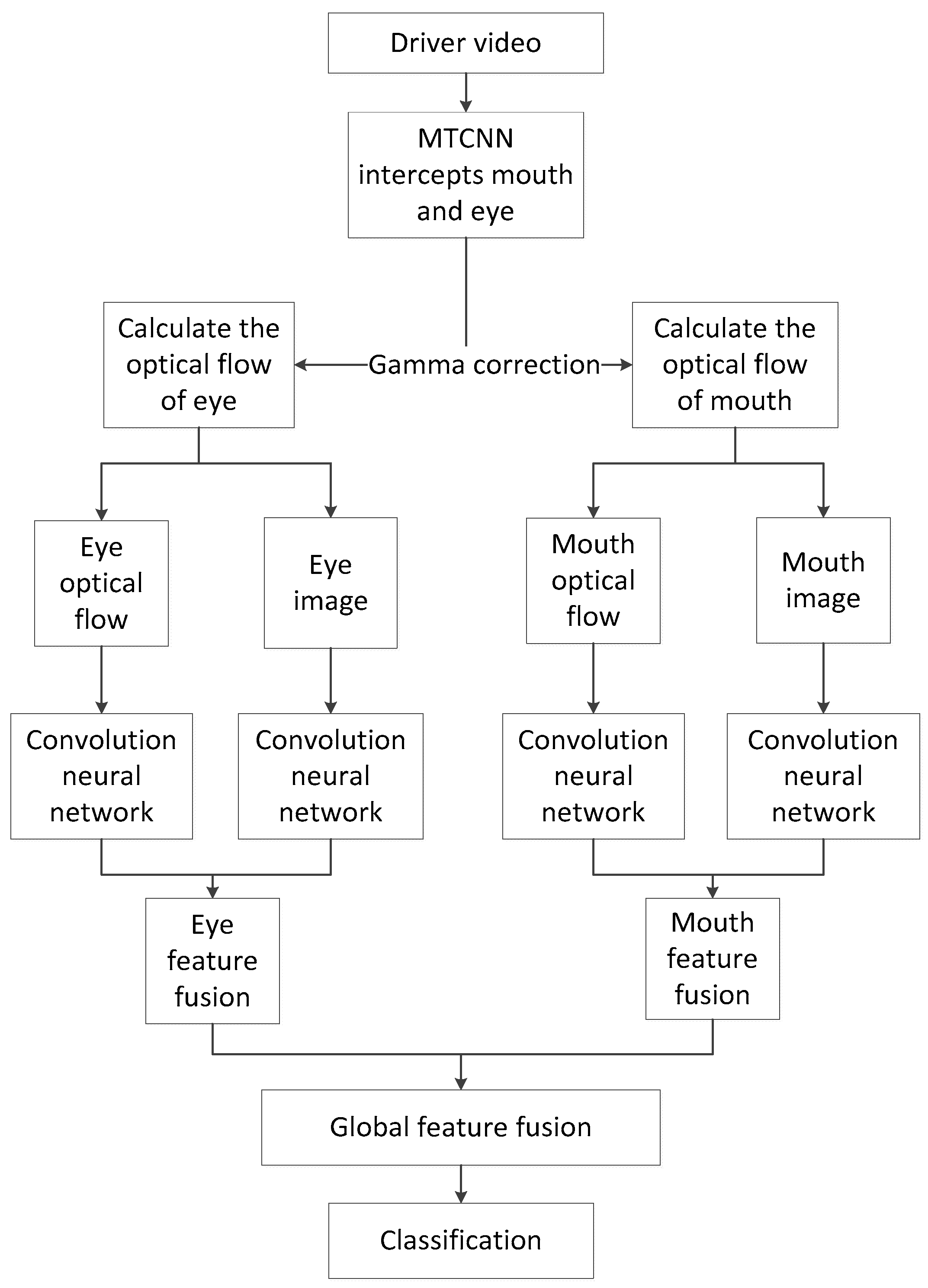
In this paper, we proposed a method using multi-task cascaded convolutional neural networks (MTCNNs) to extract the mouth and the left eye area, and use gamma correction to enhance the image contrast. Combining optical flows of the mouth and the left eye regions, we used convolutional neural network (CNN) to extract features for driver fatigue detection, which achieved good results on the National Tsing Hua University Driver Drowsiness Detection dataset (NTHU-DDD) [26]. Our algorithm flowchart is shown in Figure 1.

2.1. Face Detection and Key Area Positioning

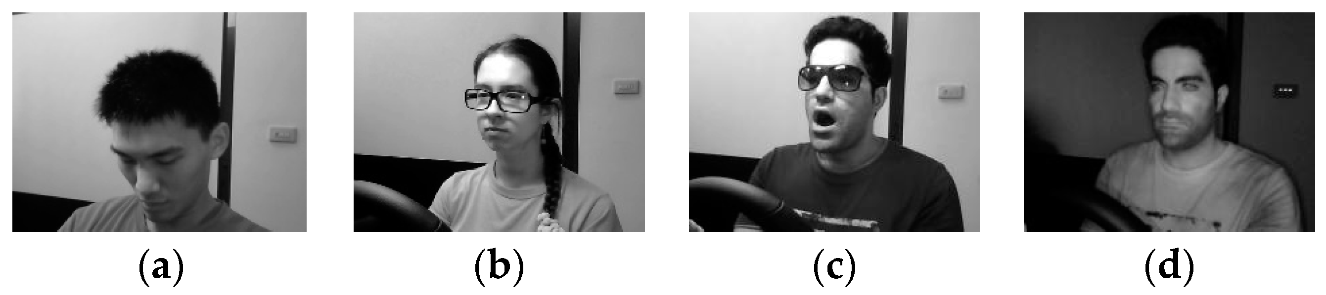
Driver fatigue detection in real driving videos can be challenging because faces are affected by many factors such as the lighting conditions and the driver’s gender, facial gestures, and facial expressions, etc. However, low-cost in-car cameras can only take low-resolution videos. Therefore, a high-performance face detector was needed. Even with a specific face area, positioning of the mouth and eye area was also very important, which contained important fatigue characteristics of the driver.

The Adaboost face detection algorithm [27], based on Haar features of the face, is not effective enough in a real, complex environment. It also cannot determine the eye area and mouth area. MTCNN [28] is known as one of the fastest and most accurate face detectors. With a cascading structure, MTCNN can jointly achieve rapid face detection and alignment. As a result of face detection and alignment, MTCNN obtained the facial bounding box and facial landmarks. In this paper, we used MTCNN for face detection and face alignment tasks.

MTCNN consists of three network architectures (P-Net, R-Net, and O-Net). In order to achieve scale invariance, the given image was scaled to different scales to form an image pyramid. In the first stage, shallow CNNs quickly generated candidate windows; in the second stage, more complex CNNs filtered candidate windows and discarded a large number of overlapping windows; in the third stage, more powerful CNNs were used to decide whether the candidate window should be discarded, while displaying five facial key positionings.

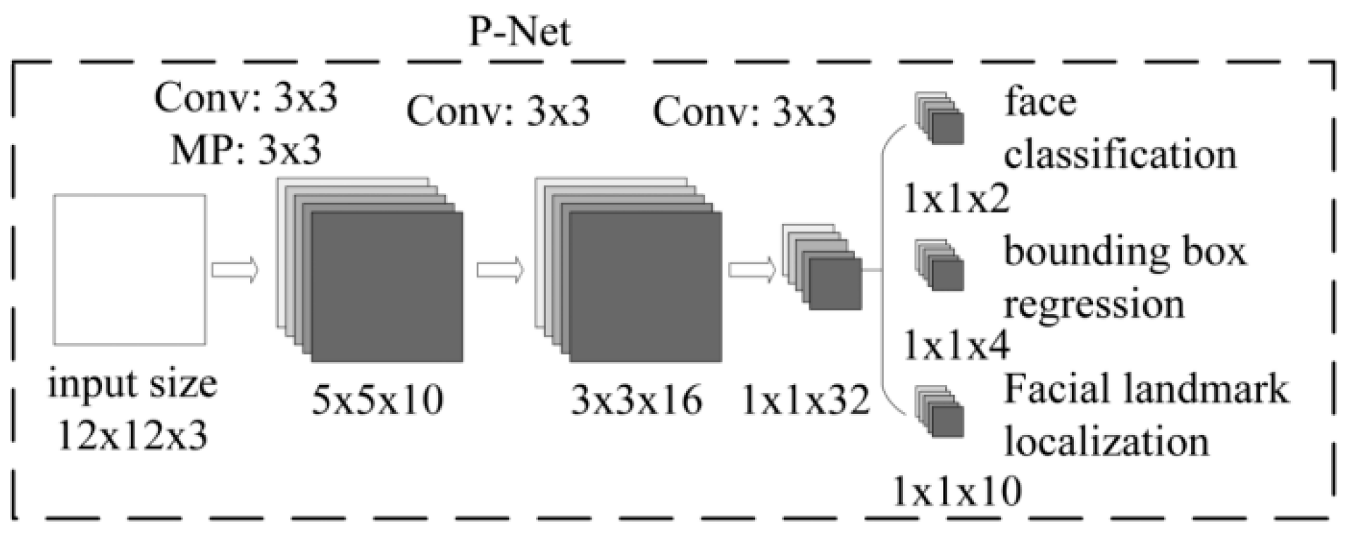
Proposal Network (P-Net) (shown in Figure 2): The main function of this network structure was to obtain the regression vector of the candidate window and bounding box in the face area. At the same time, it used the bounding box to do the regression and calibrate the candidate window, and then it merged the highly overlapping candidate boxes by non-maximum suppression (NMS). All input samples were first resized into 12 × 12 × 3, and finally the P-Net output was obtained by a 1 × 1 convolution kernel of three different output channels. P-Net output was divided into three parts: (1) face classification—the probability that the input image was a face; (2) bounding box—the position of the rectangle; and (3) facial landmark localization—the five key points of the input face sample.

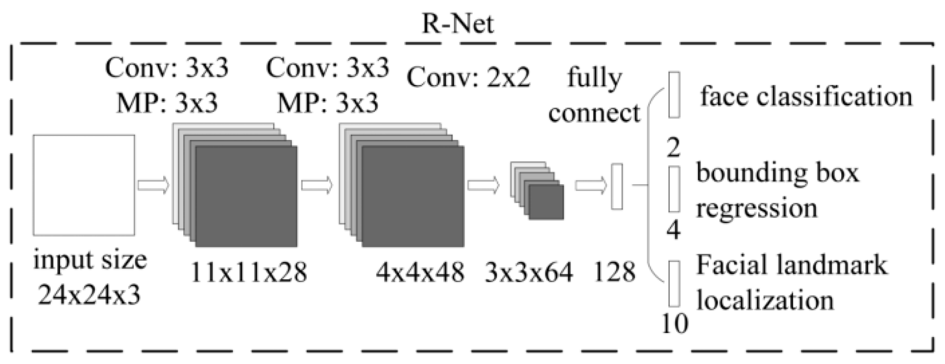
Refine Network (R-Net) (shown in Figure 3): This network structure also removed the false positive region through bounding box regression and non-maximum suppression. However, since the network structure had one more fully connected layer than the P-Net network structure, a better effect of suppressing false positives could be obtained. All input samples were first resized to 24 × 24 × 3, and finally the R-Net output was obtained by the fully connected layer. R-Net output was divided into three parts: (1) face classification—the probability that the input image was a face; (2) bounding box—the position of the rectangle; and (3) facial landmark localization—the five key points of the input face sample.

Output Network (O-Net) (shown in Figure 4): This network structure had one more convolutional layer than R-Net, so the result of the processing was finer. The network worked similarly to R-Net, but it supervised the face area and obtained five coordinates representing the left eye, right eye, nose, left part of lip, and right part of lip. All input samples were first resized to 48 × 48 × 3 dimensions, and finally the O-Net output was obtained by the fully connected layer. O-Net output was divided into three parts: (1) face classification—the probability that the input image was a face; (2) bounding box—the position of the rectangle; and (3) facial landmark localization—the five key points of the input face sample. All three networks set a threshold that represented the degree of overlap of face candidate windows in non-maximal suppression.

Compared with common detection methods such as region-based convolutional neural networks (R-CNNs) [29], MTCNN is more suitable for face detection and is greatly improved in terms of speed and accuracy.

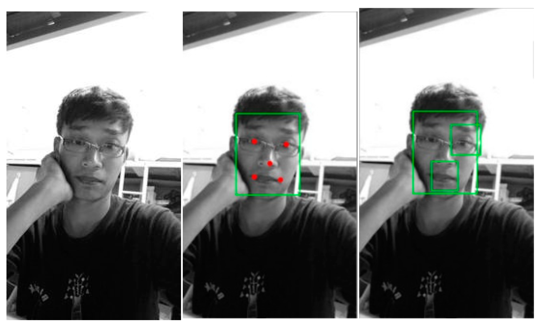
It was not adequate to determine the coordinates of the key point, thus, we needed to determine the eye and mouth area. In yawning, blinking, and other movements, mouth and eye sizes will change within a certain range. Therefore, in this paper, we used the eye coordinates as the center and the distance between the left and right part of lip as the length to determine a rectangular box for the eye area. Then, we used the midpoint between the left part of lip and the right part of lip as the center and the distance between the left part of lip and the right part of lip as the length to define a rectangular box for the mouth area. The actual effect is shown in Figure 5.

2.2. Gamma Correction

In actual scene image acquisition, the image may be overexposed or underexposed due to environmental factors such as light exposure, resulting in non-uniform gray-level distribution. This will deteriorate the image quality and negatively affect the result of the calculation.

In digital image processing, gamma correction [30] is usually applied to the correction of the output image of the display device. Since Cathode Ray Tube (CRT), Light Emitting Diode (LED), and other display devices do not work in a linear manner when displaying colors, color output in the program will eventually have diminished brightness when outputted to the monitor. This phenomenon can affect the quality of the image when calculating lighting and real-time rendering, so the output image needs gamma correction. The gray value of the input image was non-linearly transformed by gamma correction. It improved the image contrast through detecting the dark part and the light part in the image signal and increased the ratio between these two parts.

In order to utilize the gray information of the image more effectively, we gamma-corrected the input image to reduce the influence of the non-uniform gray-level distribution of the image. Since the eye and the mouth captured from image through the MTCNN were a small area with almost no partial overexposure or partial underexposure, it was possible to subject the entire obtained eye and mouth image to gamma correction, which improved image contrast.

According to the gamma correction formula, the corresponding relationship between the input pixel ${{\displaystyle P}}_{in}·$, the output pixel ${{\displaystyle P}}_{out}$, the gamma coefficient $gamma$, and the gray level $scale$ is:

$${{\displaystyle P}}_{out}={{\displaystyle \left(\frac{{{\displaystyle p}}_{in}}{scale}\right)}}^{gamma}\times scale$$

(1)

It can be deduced from (1) that, given the input pixel ${{\displaystyle P}}_{in}$, the expected output pixel ${{\displaystyle P}}_{hope}$, the gray level $scale$, we can find:

$$gamma={{\displaystyle \log }}_{\frac{{{\displaystyle P}}_{hope}}{scale}}\frac{{{\displaystyle P}}_{in}}{scale}$$

(2)

Formula (2) was relative to a single pixel. When faced with an image, a single pixel of the above formula was replaced by a grayscale mean of one image. The relationship between the gray mean ${{\displaystyle P}}_{mean}$ and the number of pixels $n$ is:

$${{\displaystyle \left({{\displaystyle P}}_{mean}\right)}}^{gamma}\approx \frac{{\displaystyle \sum _i^n{{\displaystyle \left({{\displaystyle P}}_i\right)}}^{gamma}}}{n}$$

(3)

Since it was almost impossible for every pixel of an image to be equal, the above formula should be an approximately equal sign.

As shown in Figure 6, through gamma correction, the gray value of the different input images were transformed into a roughly similar desired gray value given by us.

2.3. Optical Flow Calculation

In real, three-dimensional space, the physical concept that describes the state of motion of an object is motion field. In the space of computer vision, the signal received by the computer is often two-dimensional image information. Because one dimension of information was lacking, it was no longer suitable for us to use motion fields to describe motion state. The optical flow field was used to describe the movement of three-dimensional space objects in the two-dimensional image, reflecting the motion vector field pixel.

As indicators of driver fatigue, yawning, blinking, etc. are not a static state but a dynamic action. Therefore, just a static image was not enough. By utilizing the change of pixels over time in the image sequence and the correlation between adjacent frames, optical flow was determined based on the corresponding relationship between the previous frame and the current frame, and it contained the dynamic information between adjacent frames. Unlike the method of using continuous frames for action recognition, such as LSTM and 3D-CNN, we used the dynamic information contained in optical flow data to replace the dynamic information provided by successive frames. In this paper, we fused the features of static and dynamic information to make driver fatigue detection better than using only static images.

Optical flow is observed in the imaging plane, and it is the instantaneous velocity of the pixel motion of an object moving through space. It uses the change in pixels over time in the image sequence and the correlation between adjacent frames to find the corresponding relationship between the previous frame and the current frame, then it calculates the motion information of objects between adjacent frames. Suppose there is a vector set $(x,y,t)$ in every moment, which represents the instantaneous velocity of the specified coordinate $(x,y)$ at the moment of $t$. Let $I(x,y,t)$ represent the pixel brightness of point $(x,y)$ at the moment of $t$, and in a very short period of time $\Delta t$, ($x$, $y$) increases ($\Delta x$, $\Delta y$) respectively, thus, we can get:

$$\begin{array}{l}I(x+\Delta x,y+\Delta y,t+\Delta t)=\\ I(x,y,t)+\raisebox{1ex}{$\partial I$}\!\left/ \!\raisebox{-1ex}{$\partial x$}\right.\Delta x+\raisebox{1ex}{$\partial I$}\!\left/ \!\raisebox{-1ex}{$\partial y$}\right.\Delta y+\raisebox{1ex}{$\partial I$}\!\left/ \!\raisebox{-1ex}{$\partial t$}\right.\Delta t\end{array}$$

(4)

At the same time, taking into account that the displacement of two adjacent frames is short enough, represented by:

$$I(x,y,t)=I(x+\Delta x,y+\Delta y,t+\Delta t)$$

(5)

we get:

$$\raisebox{1ex}{$\partial I$}\!\left/ \!\raisebox{-1ex}{$\partial x$}\right.\Delta x+\raisebox{1ex}{$\partial I$}\!\left/ \!\raisebox{-1ex}{$\partial y$}\right.\Delta y+\raisebox{1ex}{$\partial I$}\!\left/ \!\raisebox{-1ex}{$\partial t$}\right.\Delta t=0$$

(6)

$$\raisebox{1ex}{$\partial I$}\!\left/ \!\raisebox{-1ex}{$\partial x$}\right.\raisebox{1ex}{$\Delta x$}\!\left/ \!\raisebox{-1ex}{$\Delta t$}\right.+\raisebox{1ex}{$\partial I$}\!\left/ \!\raisebox{-1ex}{$\partial y$}\right.\raisebox{1ex}{$\Delta y$}\!\left/ \!\raisebox{-1ex}{$\Delta t$}\right.+\raisebox{1ex}{$\partial I$}\!\left/ \!\raisebox{-1ex}{$\partial t$}\right.\raisebox{1ex}{$\Delta t$}\!\left/ \!\raisebox{-1ex}{$\Delta t$}\right.=0$$

(7)

Since:

$$\raisebox{1ex}{$\Delta x$}\!\left/ \!\raisebox{-1ex}{$\Delta t$}\right.=v_x,\raisebox{1ex}{$\Delta y$}\!\left/ \!\raisebox{-1ex}{$\Delta t$}\right.=v_y$$

(8)

The final conclusion can be drawn as:

$$\raisebox{1ex}{$\partial I$}\!\left/ \!\raisebox{-1ex}{$\partial x$}\right.v_x+\raisebox{1ex}{$\partial I$}\!\left/ \!\raisebox{-1ex}{$\partial y$}\right.{{\displaystyle v}}_y+\raisebox{1ex}{$\partial I$}\!\left/ \!\raisebox{-1ex}{$\partial t$}\right.=0$$

(9)

where $v_x$, $v_y$ is the speed of $x$, $y$ respectively, which is called the optical flow of $I(x,y,t)$.

The Farneback algorithm [31] is a method of calculating dense optical flow. First of all, it approximates each neighborhood of two frames with a second-degree polynomial, which can be done efficiently with polynomial expansion transformations. Next, by observing how an exact polynomial transforms under translation, a method of estimating the optical flow is derived from the polynomial expansion coefficients. With this dense optical flow, image registration at the pixel level is possible. Consequently, the effect of registration is significantly better than that of sparse optical flow registration.

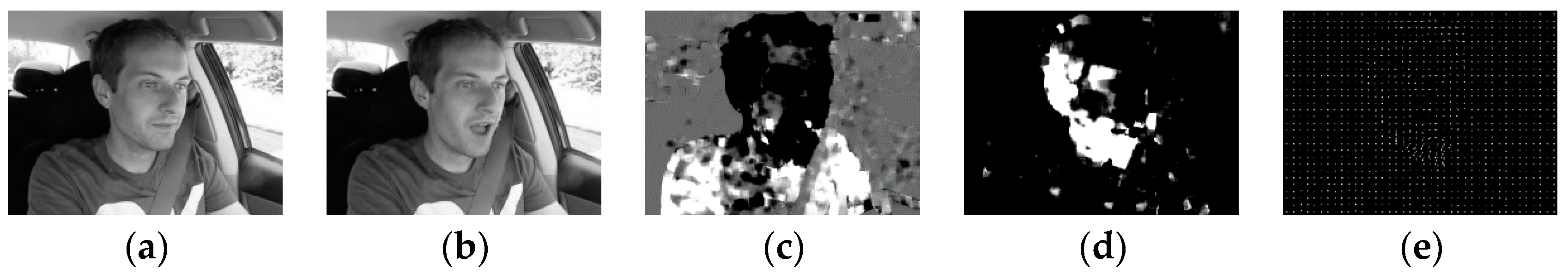
During car driving, noting that the camera is fixed in the car, the driver’s face optical flow is generated by the driver’s face movement in the scene. In order to reflect the driver’s dynamic face changes, we used the Farneback algorithm to calculate the dense optical flow between adjacent frames of left eye and mouth respectively, which is shown in Figure 7.

2.4. Fatigue Detection

CNN, which avoids complicated pre-processing of the image, can extract features with its special structure of local connection and weight sharing by directly inputting the original image. It has unique advantages in image processing.

Videos can be decomposed into spatial and temporal parts. The spatial part refers to appearance information of the independent frame, and the temporal part refers to motion information between two frames. The network structure proposed by reference [31] consisted of two deep networks, which handled the dimensionality of time and space separately. The video frame was sent to the first CNN to extract static features; meanwhile, the optical flow extracted from the video was sent to another CNN to extract dynamic features. Finally, the scores from the softmax layers of both networks were merged.

As a result of the natural state, the motion states of the left and right eyes of a person were consistent. Reddy et al. [24] proposed a method of driver drowsiness detection through inputting only the mouth region and the left eye region of a human face into the network. Compared with face inputs, this algorithm not only simplified the input but also achieved better results.

Our algorithm first performed face detection of the driver. Then, the left eye area and the mouth area were intercepted into the fatigue detection network, combined with the optical flow image of the left eye and mouth, and the driver was judged whether they were in a normal, speaking, yawning, or dozing state. Unlike using LSTM and 3D-CNN to capture motion sequences from video frames to classify action, we used CNN to extract static features from the original image and dynamic features from the optical flow, thereby classifying a short time action.

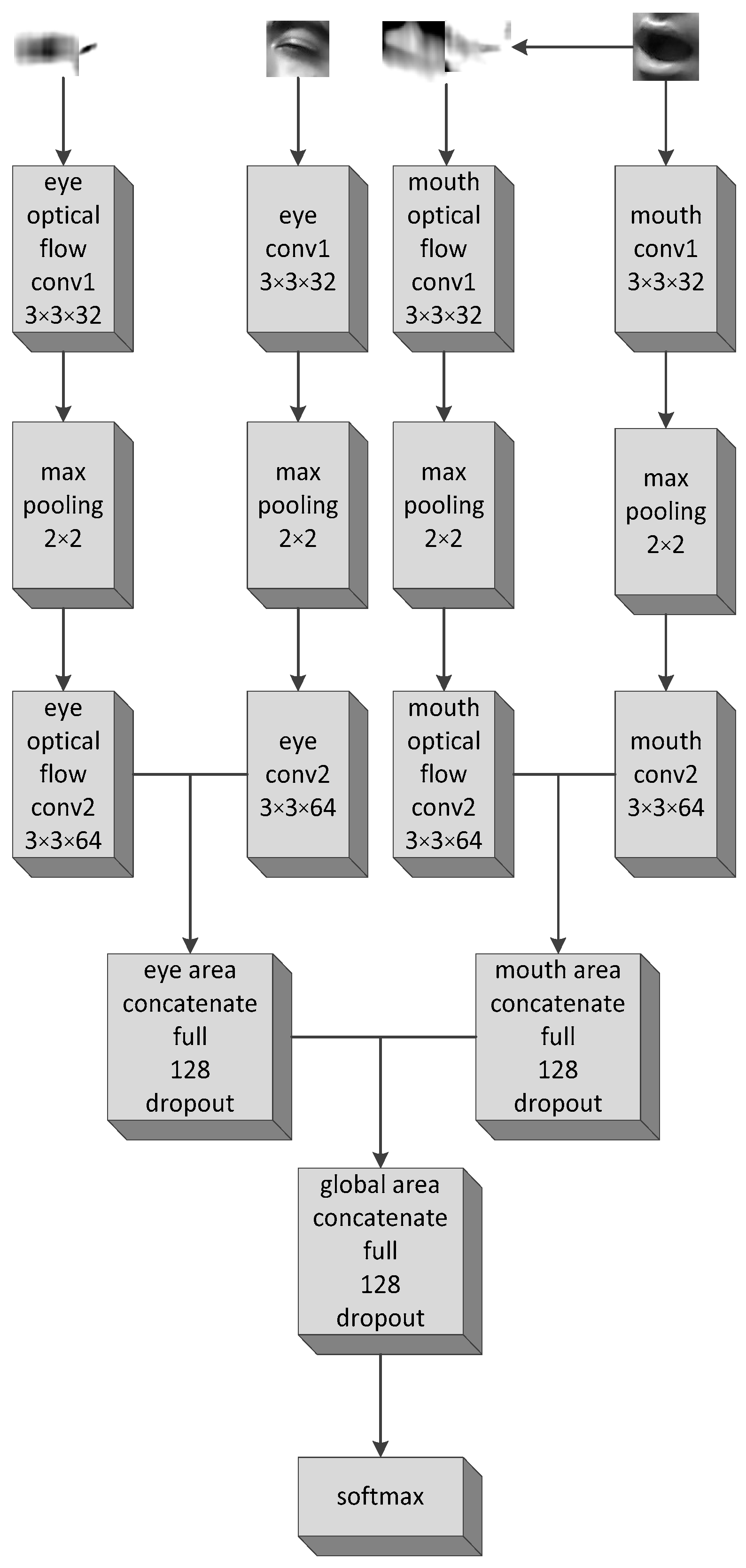
The fatigue detection network, as shown in Figure 8, included four subnetworks. Input images in each sub-network were first resized to 50 × 50 × 3 dimensions. The first subnetwork was to extract the feature of optical flow of the left eye. The second sub-network was to extract the feature of the left eye. The third sub-network was to extract the feature of optical flow of the mouth. The fourth sub-network was to extract the feature of the mouth. Together with the mouth and eye areas obtained after detection and interception, the calculation results of the optical flow of the mouth and eye areas were respectively inputted into the four subnetworks. After several layers of convolution and pooling, the left eye subnetwork and the left eye optical flow subnetwork were first fused to obtain further left eye regional features, while the mouth subnetwork and the mouth optical flow subnetwork were merged to obtain a further mouth regional feature. For the sake of obtaining global region characteristics, we merged the two new subnetworks and reintegrated them into the full connection layer. Finally, we inputted the data into the softmax layer for classification and obtained a 1 × 5 vector, which represented the probability of each class. To avoid over-fitting, an L2-regularization was added at each convolutional layer. At the same time, a dropout hyperparameter was added at each fully connected layer.

3. Experimental Results

In the following, we provide competitive experimental results on the dataset used for driver drowsiness detection and compare the performance of state-of-the-art methods.

3.1. National Tsing Hua University-Driver Drowsiness Detection (NTHU-DDD) Dataset

The NTHU-DDD dataset [25] was a dataset developed by National Tsing Hua University, which was used at the Asian Conference on Computer Vision Workshop on Driver Drowsiness Detection. The entire dataset contained 36 subjects of different ethnicities, which were recorded with and without wearing glasses/sunglasses under a variety of daytime and nighttime simulated driving conditions. All movements of the driver were captured, including normal driving, yawning, slow blink rate, falling asleep, laughing, etc. The training set contained 360 video clips of 18 subjects, while the evaluation set consisted of 20 video clips of four subjects. The dataset contained a lot of normal, drowsy, talking, and yawn face data in various scenarios. Thus, the algorithm should consider robustness in all circumstances. Some screenshots from the dataset are shown in Figure 9.

3.2. Experiment

We trained our models using a training dataset with a stratified five-fold cross-validation [32], where data folds were chosen such that each fold had nearly the same class distribution as the original dataset, and it used an evaluation dataset for the test. Images were extracted one frame from every three frames in the videos, and they were labeled into five driver states: normal, drowsiness, nodding, talking, and yawning; the distribution of these classes in the dataset was around 5:9:2:5:3. Input images were first resized to a 50 × 50 size. The model input of the experiment without gamma correction was the original image, while the model with gamma correction input images had an average gray value of 120. We developed our models using the Keras framework and run experiments on GTX 1080 Ti. All of the layer weights were randomly initialized. We chose the hyper-parameters using a grid search. The network was trained using a batch gradient descent with a batch size of 128 and a dropout rate of 0.2. An initial learning rate of 0.1 was used in the optimization function Adadelta. Training was stopped when the validation loss did not improve for 50 iterations. The model was trained for around 230 iterations. The results are shown in

Table 1. Drowsiness detection accuracies (%) for different scenarios of the NTHU-DDD dataset.

Scenarios	3D-DCNN [28]	3-nets DDD [29]	MLP [27]	seqMT-DMF [30]	Fatigue Detection Network (FDN)	Gamma Fatigue Detection Network (GFDN)
Bareface	75.10	69.83	87.12	84.46	97.18	97.36
Glasses	72.30	75.93	84.85	77.35	97.60	97.35
Sunglasses	70.90	69.86	75.11	86.43	97.13	97.86
Night-bareface	68.40	74.93	81.40	82.48	94.03	96.25
Night-glasses	68.30	74.77	76.15	87.18	94.26	96.14
Average	71.20	73.06	80.93	83.44	96.60	97.06

and

Table 2. Drowsiness detection accuracies (%) for different states of the NTHU-DDD dataset in GFDN and derived models.

State	GFDN-K-Nearest Neighbor (KNN)	GFDN-Centroid Displacement-Based K-Nearest Neighbor (CDNN)	GFDN-Support Vector Machine (SVM)	GFDN-Random Forest (RF)	GFDN
normal	92.86	93.42	93.96	94.61	93.70
drowsiness	98.02	97.93	98.05	97.49	98.11
nodding	96.00	96.11	96.51	96.21	96.31
talking	97.37	97.02	97.18	96.83	97.75
yawning	97.19	97.21	97.44	97.25	97.84
Average	96.67	96.78	96.98	96.70	97.06

.

We tested the model at four different levels: (1) different scenarios; (2) different driving states; (3) different derived models; (4) average performance. Performances of the models without gamma correction, fatigue detection network (FDN), and with gamma correction, gamma fatigue detection network (GFDN), were comparable to state-of-the-art methods. In Table 1, we showed a comparison with state-of-the-art methods. Our models outperformed the existing methods in all of the scenarios, and the average performance surpassed all the state-of-the-art methods, which achieved a 97.06% accuracy. In addition, GFDN increased accuracy by 2% compared to FDN in a night environment.

We showed another result in Table 2. We obtained features before the softmax layer in the GFDN model as inputs, and we tested them with other classifiers. We chose and tuned four classification algorithms including k-nearest neighbors (KNNs) [33], centroid displacement-based k-nearest neighbors (CDNNs) [34], support vector machine (SVM) [35], and random forest (RF) [36]. Parameter k was tuned and chosen to be five and three in KNN and CDNN, respectively, through cross-validation. It was shown below that the accuracy of each derived model dropped slightly.

Considering the problem of unbalanced data, we added an F1-score to evaluate metrics.

Table 3. Drowsiness detection details for different states of the NTHU-DDD dataset in GFDN.

Real	Predict
	Normal	Drowsiness	Nodding	Talking	Yawning
normal	9643	269	24	331	24
drowsiness	164	21,234	112	12	121
nodding	11	183	5833	23	6
talking	204	9	39	12,614	38
yawning	15	167	19	19	9970

shows the details in predicting different states using the GFDN model. According to Table 3 we could obtain the precision rate and the recall rate, which are shown in

Table 4. Precision rate and recall rate (%) for different states.

	Normal	Drowsiness	Nodding	Talking	Yawning
Precision Rate	96.07	97.12	96.78	97.03	98.13
Recall rate	93.70	98.11	96.31	97.75	97.84

. Based on this, the F1-score was calculated to be 0.9688.

4. Discussion

In this paper, we employed two-stream networks, multi-facial features, and gamma correction for driver fatigue detection. Gamma corrections in the input image, input partial facial features, and fused dynamic information resulted in more accurate driver fatigue detection compared to existing methods. The experiment results showed that our GFDN model had an average accuracy of 97.06% on the NTHU-DDD dataset.

It is not suitable to directly input the entire image, which contains extraneous information. The driver’s face is only about 200 × 150 pixels, compared with the actual 640 × 480 image in the camera shot. The full image contains useless information and has a negative effect on classification. Furthermore, after the image is resized and sent to CNN, it carries much less correlative information, which makes it difficult to learn features. Inputting partial facial images can avoid inaccurate classifications. Therefore, inputting the left eye and mouth area, which are closely related to driver fatigue, is a sensible idea.

Using only static images is not accurate enough for driver drowsiness detection; this is an action recognition task instead of an image recognition task. For instance, people are opening their mouths when both yawning and speaking. There is no difference in static images, while optical flow can reflect the difference. When the mouth and left eye are used as the inputs of the network, dynamic information between the continuous frames is not used. Better results can be obtained using a two-stream neural network that contains dynamic information in optical flow.

Poor image quality caused by non-uniform gray-level distribution can have negative effects on calculation results, for example, images taken in too bright or too dark environments. In experiments, input images are subjected to gamma correction to effectively improve the accuracy, which reduces the calculation errors caused by insufficient image contrast. It brings a 2% improvement in classification accuracy in night environments.

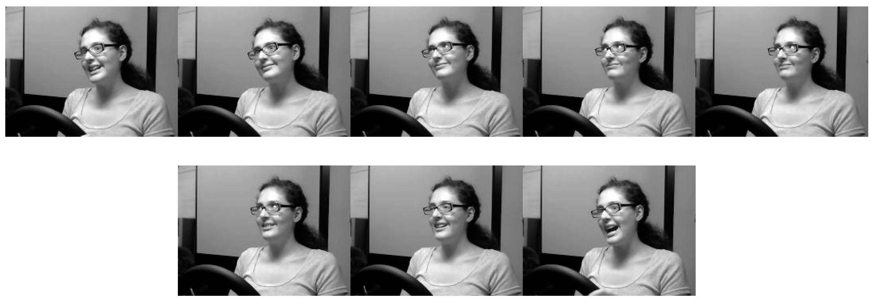
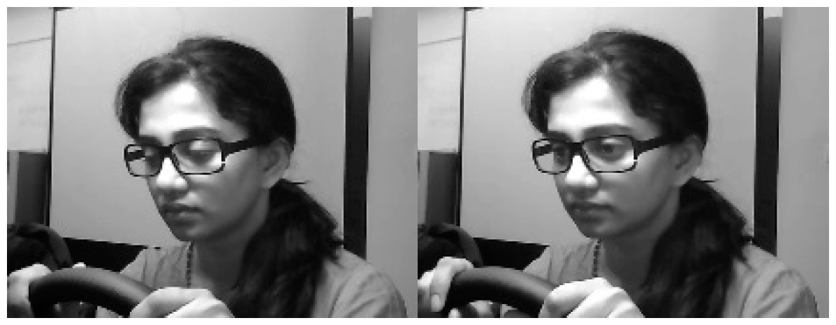
It was shown in Table 2 and Table 3 that the normal state had the worst classification accuracy among all states, and most misclassified normal images were labeled into drowsiness and talking. We further checked the dataset and found that: (1) images for the whole duration of talking were labeled as talking, as shown in Figure 10, including images that looked like the normal state; (2) some drowsiness images looked like the normal state, except minor differences in eye sleepiness, as shown in Figure 11. These increase the difficulty of model classification.

5. Conclusions

We proposed a driver fatigue detection algorithm based on multi-facial feature fusion, which not only avoided peripheral equipment on the driver’s body, but also had high accuracy. We applied CNN and optical flow to video comprehension. We focused on partial information of the face, which was closely related to driver fatigue in the algorithm. We utilized optical flow to obtain dynamic information, and we used gamma correction to enhance image contrast. Thus, we achieved a competitive accuracy. From the experimental results, we can see that our model outperforms state-of-the-art methods.