A Novel Self-Adaptive VM Consolidation Strategy Using Dynamic Multi-Thresholds in IaaS Clouds

Abstract

With the rapid development of cloud computing, the demand for infrastructure resources in cloud data centers has further increased, which has already led to enormous amounts of energy costs. Virtual machine (VM) consolidation as one of the important techniques in Infrastructure as a Service clouds (IaaS) can help resolve energy consumption by reducing the number of active physical machines (PMs). However, the necessity of considering energy-efficiency and the obligation of providing high quality of service (QoS) to customers is a trade-off, as aggressive consolidation may lead to performance degradation. Moreover, most of the existing works of threshold-based VM consolidation strategy are mainly focused on single CPU utilization, although the resource request on different VMs are very diverse. This paper proposes a novel self-adaptive VM consolidation strategy based on dynamic multi-thresholds (DMT) for PM selection, which can be dynamically adjusted by considering future utilization on multi-dimensional resources of CPU, RAM and Bandwidth. Besides, the VM selection and placement algorithm of VM consolidation are also improved by utilizing each multi-dimensional parameter in DMT. The experiments show that our proposed strategy has a better performance than other strategies, not only in high QoS but also in less energy consumption. In addition, the advantage of its reduction on the number of active hosts is much more obvious, especially when it is under extreme workloads.

1. Introduction

Infrastructure as a Service (IaaS) has been very popular in the cloud computing area over the past few years. Popular IaaS cloud providers, such as Rackspace and Amazon EC2, are delivering these virtual resources to customers in different data centers over the Internet. However, due to the huge demand for cloud computing, thousands of large-scale cloud computing centers have been established, which leads to a great deal of power consumption [1]. The main reason of such high energy consumption is not the power consumption by large quantities of hardware, but the inefficient usage of these cloud resources. Therefore, trying to develop adaptive strategies to dynamically adjust each resource in cloud data centers is very important from an energy-efficiency perspective.

One of the solutions for improving energy efficiency is to leverage the capabilities of virtualization technology [2], which improves the efficiency of resource utilization by sharing a physical machine(PM) among multiple virtual machines (VMs). The live migration [3] of virtual machine to dynamically scheduled resource can transfer VMs from one PM to another, while keeping the services provided by the corresponding VM still available. This technique makes it possible to dynamically optimize the placement of VMs in the different purpose of energy efficiency [4] or load balance [5], according to the resource usage at any time.

The key mechanism to improve energy efficiency in cloud data centers is called VM consolidation [6], which aims at migrating VMs into a lower number of PMs to increase the utilization of resources in cloud data centers. However, in some scenarios, packing too many VMs into one single PM may lead to poor Quality-of-service (QoS); since VMs on one PM always share the same underlying physical resources. Therefore, VM consolidation strategies, designed to dynamically adjust VMs’ placement, should comprehensively ensure reliable QoS, which is often defined via Service Level Agreements (SLAs) [7]. Besides, energy consumption [8] and VM migration costs [1] during each VM consolidation step should also be taken into consideration.

Threshold-based strategy [6] uses upper and lower threshold to select proper source PM, which is often considered as the first step of VM consolidation. The key point of these threshold-based strategies can be concluded as comparing each PM’s current status with the defined threshold that is either static or adaptive [1]. Although researches on static threshold [9] show that set 0.6 as the upper threshold of CPU utilization could achieve a better performance in energy consumption and VM migrations, it still cannot achieve good performance in SLA violation, due to the dynamic resource usage in an IaaS environment.

Different from static method, adaptive threshold strategy can leverage the real-time usage of different resource to dynamically adjust its threshold. Most of the existing studies [1,4,9,10] only consider one resource demand such as CPU utilization while ignoring other infrastructure resource requests like memory or bandwidth, etc. However, the resource requirement of different workloads, like computing-intensive, input and output (I/O)-intensive or hybrid-intensive, are very diverse [5], as computing-intensive workloads usually call for more CPU/RAM resources, while I/O-intensive workloads prefer consuming more network bandwidth. Besides, selecting a VM only based on one resource will cause saturation in terms of this resource and can lead towards no further improvement in utilization with other types of resources underutilized [11].

Based on that, we propose a novel self-adaptive VM consolidation strategy based on the dynamic multi-thresholds adjustment mechanism, which is conducted by comparing the predicted future requests of each multi-dimensional infrastructure resources with their current environment status. The dynamic multi-thresholds are used for PM selection, as the first step in VM consolidation. In addition, an improved VM selection algorithm and a modified VM allocation algorithm are proposed, each of which belongs to the next two steps of VM consolidation. Our contributions of this work are as follows:

(1)

We define each parameter of our proposed multi-thresholds, as well as a dynamic adjustment mechanism for these parameters. The selection of each overload or underload PM (source PM) based on the multi-thresholds strategy can perfectly meet different VM consolidation requests.

(2)

We improve the VM selection algorithm MW-MVM (multi-weight VM migration) by utilizing the multi-dimensional parameters of our proposed multi-dynamic threshold. The selection of target VM based on this algorithm can get a better performance in migration costs and energy consumption.

(3)

We modify the VM placement algorithm MW-BF (multi-weight Best Fit) for the allocation of target migration VMs and new VMs requested by users on physical nodes. The experiments show that our modified algorithm can efficiently reduce SLA violation, as well as the number of active hosts.

2. Preliminaries

2.1. Virtual Machine Consolidation

The procedure of VM consolidation can be comprised of three core components: (1) Source PM selection, (2) Target VM selection and (3) VM placement. In (1), a set of PMs are selected for VMs to migrate out. This component takes all the PMs and VMs as input and selects one or more PMs as the source PM. In (2), one or more VM(s) are selected from a source PM for migration. This component takes the source PM as input which has been selected by step (1) and is going to select one or more VMs from this PM to a different PM. In (3), a PM is selected to hold the VM selected from (2) or the new VM requests.

As portrayed in Figure 1, VMs are scattered in multiple PMs before VM consolidation is applied, with PM 2 only holding one VM while PM 1 holds 5 VMs at high overload. On one side, PMs at overload status can easily cause high SLA violation. On the other side, underloaded PM 2 with only one VM in it still needs to remain alive, which increases unnecessary energy costs. Therefore, if no VM consolidation strategy is interposed to the inefficient usage of computing resources, much extra energy will be wasted, as well as lower QoS.

Based on different threshold strategies of VM consolidation, the status of each PM can be divided as overload, moderate or underload. If a PM is defined as underload, then all VMs within it would be migrated out and it will then be set to the sleep mode or shut down to reduce energy costs (PM 2). While VMs in the moderate PM will not be migrated, this PM would become one of the target PMs for some VMs to migrate in (PM 3). Besides, in order to prevent a potential high SLA violation, an overload PM would migrate some selected VMs to others (PM 1). Therefore, after adding VM consolidation strategy, there are only two servers alive in the system an both of them are at moderate status. In addition, the underload server (PM 2) is shut down, which further decreases the energy consumption.

2.2. System Architecture

We consider that the cloud data center in this paper contains m heterogeneous PMs, $\mathrm{PM}=\langle PM\left(1\right),PM\left(2\right), \dots , PM\left(m\right)\rangle$. Each PM consists of a local manager, a Virtual Machine Monitor (VMM), some virtual machines and their physical resources, such as CPU, RAM and Network bandwidth. The VMM in every local host (Figure 2) are used to supervise their real-time status, as different VM consolidation strategies can be operated within each VMM by the contact of global manager and local manager, yet without any manual adjustment.

• User submit request of the Infrastructure resource on the cloud, including CPU, RAM, etc.
• The global manager collects information from local ones to maintain the whole system resource utilization.
• The global manager optimizes of the placement of VM in reference of VM consolidation strategy, as well as the whole system status.
• The local managers resize VMs according to their resource needs and decide when and which of the selected VMs should be migrated out.
• VMMs in each node execute the operation of resizing and migrating to VMs, as well as the adjustment of their power states.

After repeating these steps, all nodes in this cloud data center can be optimized by different user-defined consolidation strategies. Most of the idle nodes are then kept switched off, whereas some temporary nodes are kept in sleep mode (or shut down) to allow the system to rapidly respond to load peaks.

2.3. Formulations and Assumptions

Let us consider that a large cloud data center provides cloud resources in the form of virtual machine instances. Usually, there are three main steps for VM consolidation: Source PM selection, Target VM selection and Target PM selection. For the first step of selecting Source PM, threshold-based method is used to determine whether a PM is overloaded or underloaded. If a PM is considered to be overloaded, which means its resource utilization is over the corresponding upper threshold, then it will be selected as the Source PM and some potential VMs in it will be migrated out to maintain the QoS; if a PM is determined to be underloaded based on the comparation of lower threshold, then all VMs in this PM will be migrated out to minimize energy consumption.

To formulate the problem (

Table 1. Notations and descriptions.

Notations	Descriptions
$VM\left(i\right)$	The $i_{th}$ VM (virtual machine), $i\in \left[1,m\right]$
$PM\left(j\right)$	The $j_{th}$ PM (physical machine), $j\in \left[1,n\right]$
$P{M}_{List}$	list of all PMs
$V{M}_{List}$	list of all VMs on $PM\left(j\right)$
$P_j^{\ast }$	utilization ratio on $PM\left(j\right)$ of parameter *
$V_i^{\ast }$	utilization ratio on $VM\left(i\right)$ of parameter *
$t_{\ast }$	current lower threshold on parameter *
$T_{\ast }$	current upper threshold of parameter *
$U_{pmj}^{\ast }$	allocated resource * on $PM\left(j\right)$
$C_{pmj}^{\ast }$	total capacity of resource * on $PM\left(j\right)$
$U_{p_j{v}_i}^{\ast }$	allocated resource * on $\mathrm{V}M\left(i\right)$ of $PM\left(j\right)$
$R_{p_j{v}_i}^{\ast }$	request resource * on $\mathrm{V}M\left(i\right)$ of $PM\left(j\right)$
$P_j$	all resource utilization ratio on $PM\left(j\right)$
$W_{VM}$	migrate weights of all VMs on $PM\left(j\right)$
$W_{PM}$	allocate weights of all PMs
$Sourc{e}_{PM}$	PMs need to execute migration
$Selec{t}_{VM}$	list of selected VMs to migrate out
$Targe{t}_{PM}$	list of target PMs to migrate in

* can represent CPU(c), RAM(r) or Bandwidth(b).

), a physical server can be uniquely identified in the form of $PM\left(j\right)=\langle V{M}_{List}, P_j, Status\rangle$, where: $V{M}_{List}$ is the list of all VMs on $PM\left(j\right)$; $P_j$ represents all resource utilization ratio on $PM\left(j\right)$ and can be divided into different kinds of resources of CPU, RAM and network bandwidth in the form of $\langle P_j^c, P_j^r, P_j^b\rangle$; Status shows the current workload of this PM, such as overloaded, moderate or underloaded; and j the unique identifier of a server which arrange from 1 to $n$. Thus, we can denote $m$ active servers in a cloud center as $PM=\langle PM\left(1\right), PM\left(2\right), \dots , PM\left(m\right)\rangle$. Similarly, the VM instance is represented in the form of $VM\left(i\right)=\langle PM\left(j\right),V_j \rangle$, where $PM\left(j\right)$ shows the PM where this VM belongs to, $V_j$ represents each resource utilization on it, and i is the unique id of a VM which arrange from 1 to $m$.

In this paper, what we mainly focus on is to propose a novel strategy for VM consolidation, aiming at saving much energy consumption and reaching high QoS. While in the process of virtual machine integration, a frequent and indispensable step is VM migration, which will affect the actual computing of resource utilization in each PM to some extent. Thus, we made the following assumptions of VM migration in the process of our consolidation strategy:

Assumption 1: The VM selected to execute migration does not cause significant resource consumption during its migration process.

Assumption 2: The time for the dynamic migration of VMs is not counted to compare the efficiency of different strategies.

For Assumption 1, in view of the numerous details in the process of VM migration, many scholars specialize in this area to research efficient strategy for dynamic VM migration. Yet this article does not consider too much detail of it and we mainly focus on the VM consolidation strategies. For Assumption 2, the length of the migration time of the each VM is not used as the standard for comparing the advantages or disadvantages of different strategies, as there is no correlation between migration time and consolidation strategies. Based on that, when we calculate the cost of VM migration, we mainly consider the number of VM migrations as an important basis to measure the merits of different consolidation strategies, and the following section will describe more details of our proposed VM consolidation strategy.

3. Novel Self-Adaptive VM Consolidation Strategy

3.1. Dynamic Multi-Thresholds (DMT)

As mentioned earlier, different types of applications may share one physical resources, fixed thresholds are not suitable for environments with dynamic workloads. Thus, the system should adaptively adjust its behavior by considering different system workloads. Based on that, we propose a novel adjustment mechanism for threshold-based VM consolidation by comparing the current threshold of each defined parameter with their future value, which is predicted by forecasting each VM’s future utilization on CPU, RAM and Network bandwidth. To further efficiently minimize the consumption of energy during each consolidation, two other parameters of SLA and VM migration costs are taken into consideration. Thus, our proposed dynamic multi-thresholds can be represented as follows:

$$T=\langle T_l, T_u, T_{SLA}, T_m\rangle$$

(1)

The multi-thresholds $T$ is defined by a combination threshold of lower utilization $T_l$, upper utilization $T_u$, SLA violation ratio $T_{SLA}$ and the number of VM migration $T_m$. Below $t_c,t_r,t_b$ represents the lower thresholds of CPU utilization ratio, RAM utilization ratio and Network bandwidth consumption, respectively, while $T_c,T_r,T_b$ represents the upper ones.

$$T_l=\langle t_c,t_r,t_b\rangle , T_u=\langle T_c,T_r,T_b\rangle$$

(2)

The adjustment of dynamic multi-thresholds to timely fit the whole cloud resources can be simplified into two main parameters, including $T_l$ and $T_u$. These two thresholds can be efficiently calculated by forecasting each future utilization ratio based on Linear Regression (Section 3.1.1). While the parameter of $T_{SLA}$ can be viewed as a limitation factor of dynamic threshold by deciding whether to change current threshold or not (Section 3.1.2). $T_m$ will be discussed to further improve the selection of VM in Section 3.2.

3.1.1. Predict Future Utilization on Linear Regression

Since the nonlinear regression has larger time and computational overhead than linear regression, which affects the overall system load to a certain extent, the value obtained by the prediction algorithm is only used as a reference for the threshold adjustment. If too much computational overhead is spent on the prediction while the subsequent adjustment mechanism is ignored, this is not conducive to the dynamic adjustment of the threshold. Based on the above concern and the experiment results, we select linear regression as our prediction algorithm and the next section will give the details of mechanism for the dynamic adjustment of the specific threshold.

As Linear Regression [12] is a popular approach to statistically estimate the relationship between different inputs and outputs, it can approximate a regression function by modeling the relationship between input and output variables in a straight line, where ${\alpha }_1$ and ${\alpha }_2$ are regression coefficients.

$$y={\alpha }_{1}x+{\alpha }_2$$

(3)

To measure the goodness of a regression function is to compare the predicted output variable ($\widehat{y}$) with the real one ($y$) in data point i, as their difference ${\epsilon }_i$ can be considered as the magnitude of the residual at each of the $\mathrm{n}$ data points.

$${\epsilon }_i=y_i-\widehat{y_i}$$

(4)

The proposed LR algorithm approximates a prediction function based on the linear regression method. The function shows the linear relationship between the future and current CPU utilization in all hosts as follows: where ${\alpha }_1$ and ${\alpha }_2$ are regression coefficient parameters, while $\widehat{p_c}$ and $p_c$ are the expected and current total CPU utilization values of all hosts, respectively.

$$\widehat{p_c}={\alpha }_1{p}_c+{\alpha }_2$$

(5)

Here ${\alpha }_1$ and ${\alpha }_2$ are calculated by estimating the $k$ last CPU utilization in all hosts. In our experiment, the value of $k$ is set to 15 in our simulation, because the interval of utilization measurements is eight minutes. The history value of each resource utilization over two hours ago is significant to forecast its short-time future utilization.

Moreover, the value obtained by the prediction algorithm is only used as a reference for the threshold adjustment, and the predicted value is not completely used as a future threshold value. Therefore, the following adjustment mechanism can be seen as a secondary selection and adjustment of the predicted value. That is to say, the dynamic adjustment mechanism of the thresholds shown in Section 3.1.2 not only considers the value predicted by linear regression obtained in this section, but also compares the current overall workload of the system.

3.1.2. DMT Adjustment Mechanism

To efficiently balance the consumption of energy cost and SLA violation, the rules of dynamically adjusting parameter $t_c$ and $T_c$ within $T_l$ and $T_u$ are restricted to SLA violation threshold $T_{SLA}$. We divided the problem into the following two situations, where the $Curren{t}_{SLA}$ can be calculated by statistic Interquartile range of SLA violation on all hosts.

• Situation 1: $Curren{t}_{SLA}<T_{SLA}$

Since the $Curren{t}_{SLA}$ is below the threshold of SLA violation (

Table 2. DMT adjustment when $Curren{t}_{SLA}<T_{SLA}$.

Predicted Utilization (if)	Threshold Adjustment (then)
$\widehat{p_c}>T_c$	$T_c= \widehat{p_c}$
$\widehat{p_c}<T_c$	$T_c$
$\widehat{p_c}<t_c$	$t_c= \widehat{p_c}$
$\widehat{p_c}>t_c$	$t_c$

), our purpose of this situation can mainly focus on energy saving. When the predicted utilization $\widehat{p_c}$ of all hosts is greater than the current threshold $T_c$ in the case of the parameter of CPU, this means that there will be many CPU requests by VMs in the future. In such a case, we choose to replace $T_c$ by $\widehat{p_c}$, since the higher the upper threshold, the less VM migration will take place and the more the energy will be saved. At the same time, when $\widehat{p_c}$ is below $T_c$, keep the previous value of $T_c$ instead of replacing. If $\widehat{p_c}$ is below the current lower threshold $T_l$ in CPU parameter $t_c$, this means that there will be fewer requests of CPU resources in the future. In such a case, we choose to replace $t_c$ by $\widehat{p_c}$, since the lower the $T_l$, the more the hosts will be switched to sleep mode to eliminate the idle power consumption, and all VMs that are on low resource utilization host will be migrated to other suitable hosts. Otherwise, keep $t_c$ as its previous value.

• Situation 2: $Curren{t}_{SLA}>T_{SLA}$

Unlike situation 1, when $Curren{t}_{SLA}$ is higher than $T_{SLA}$, this means that situation 2 has already caused much SLA violation in the current stage (

Table 3. DMT adjustment when $Curren{t}_{SLA}>T_{SLA}$.

Predicted Utilization (if)	Threshold Adjustment (then)
$\widehat{p_c}>T_c$	$T_c$
$\widehat{p_c}<T_c$	$T_c= \widehat{p_c}$
$\widehat{p_c}<t_c$	$t_c$
$\widehat{p_c}>t_c$	$t_c= \widehat{p_c}$

). Since too much SLA violation will lead to a lower QoS, the key to dealing with this problem is to reduce the workload of high load hosts. Based on the goal of dropping SLA violation, we choose to keep the previous upper value $T_c$ when $\widehat{p_c}$ is higher than $T_c$ and replace the $T_c$ of $\widehat{p_c}$ when $\widehat{p_c}$ is lower than $T_c$ because the higher upper threshold may easily lead to high SLA violation. On the other hand, when $\widehat{p_c}$ is lower than $t_c$, keeping the precious lower threshold will help prevent low load hosts from migrating all VMs to other hosts which will help reduce SLA violation. Similarly, when $\widehat{p_c}$ is higher than $t_c$, replacing $t_c$ of $\widehat{p_c}$ could drop the SLA violation and thus help improve the QoS.

For a brief description, we only take the threshold of CPU utilization ($t_c, T_c$) of all hosts as an example, showing how it dynamically adjusts its current thresholds by comparing its current value with the predicted one. Similarly, the procedure of adjusting the other two parameters of RAM ($t_r, T_r$) and Bandwidth ($t_b, T_b$) can also following these steps. Many details for selecting source PM based on this DMT are shown below.

3.1.3. Source PM Selection Based on DMT

To select a proper source PM, the first step is to detect their workload based on the comparation of each parameter in DMT (Algorithm 1).

Algorithm 1 Load Detection (LD)

1 Input: $PM\left(j\right)$ 2 Output: load_status 3 foreach $PM\left(j\right)$ in $P{M}_{List}$ 4   if (some parameter * in $PM\left(j\right)$ fit $P_j^{\ast }> T_{\ast }$) 5     load_status = 1 6   else if (all parameter * in $PM\left(j\right)$ fit $P_j^{\ast }< T_{\ast }$) 7     load_status = 2 8   else 9     load_status = 0 10 return load_status

Here we take three parameters (CPU, RAM, Bandwidth) of the whole system to reflect its total resource utilization by each PM with different numbers of virtual machines in it (Algorithm 2). For each host, if one of its parameters is over the upper threshold or all of them are below the lower threshold, it will be selected as one of the target physical machines in $Sourc{e}_{PM}$ which contains the migration list of all target hosts (Table 1). At the same time, PMs with higher SLA violation than the threshold $T_{SLA}$ will first be selected to $Sourc{e}_{PM}$, and will be set to higher priority.

Algorithm 2 Source PM Selection

1 Input: $P{M}_{List}$ 2 Output: $Sourc{e}_{PM}$ 3 foreach $PM\left(j\right)$ in $P{M}_{List}$ 4 if ($PM{\left(j\right)}_{SLA}>T_{SLA}$) then 5   $Sourc{e}_{PM}$ ← $PM\left(j\right)$ 6 else 7   if (LD ($PM\left(j\right)$) == 1) then 8     $Sourc{e}_{PM}$ ← $PM\left(j\right)$ 9     $Selec{t}_{VM}$ ← select VMs on VM selection policy 10   if (LD ($PM\left(j\right)$) == 2) then 11     $Sourc{e}_{PM}$ ← $PM\left(j\right)$ 12     $Selec{t}_{VM}$ ← all VMs in $PM\left(j\right)$ 13     set $PM\left(j\right)$ to sleep mode or switch off 14 return selected source PMs

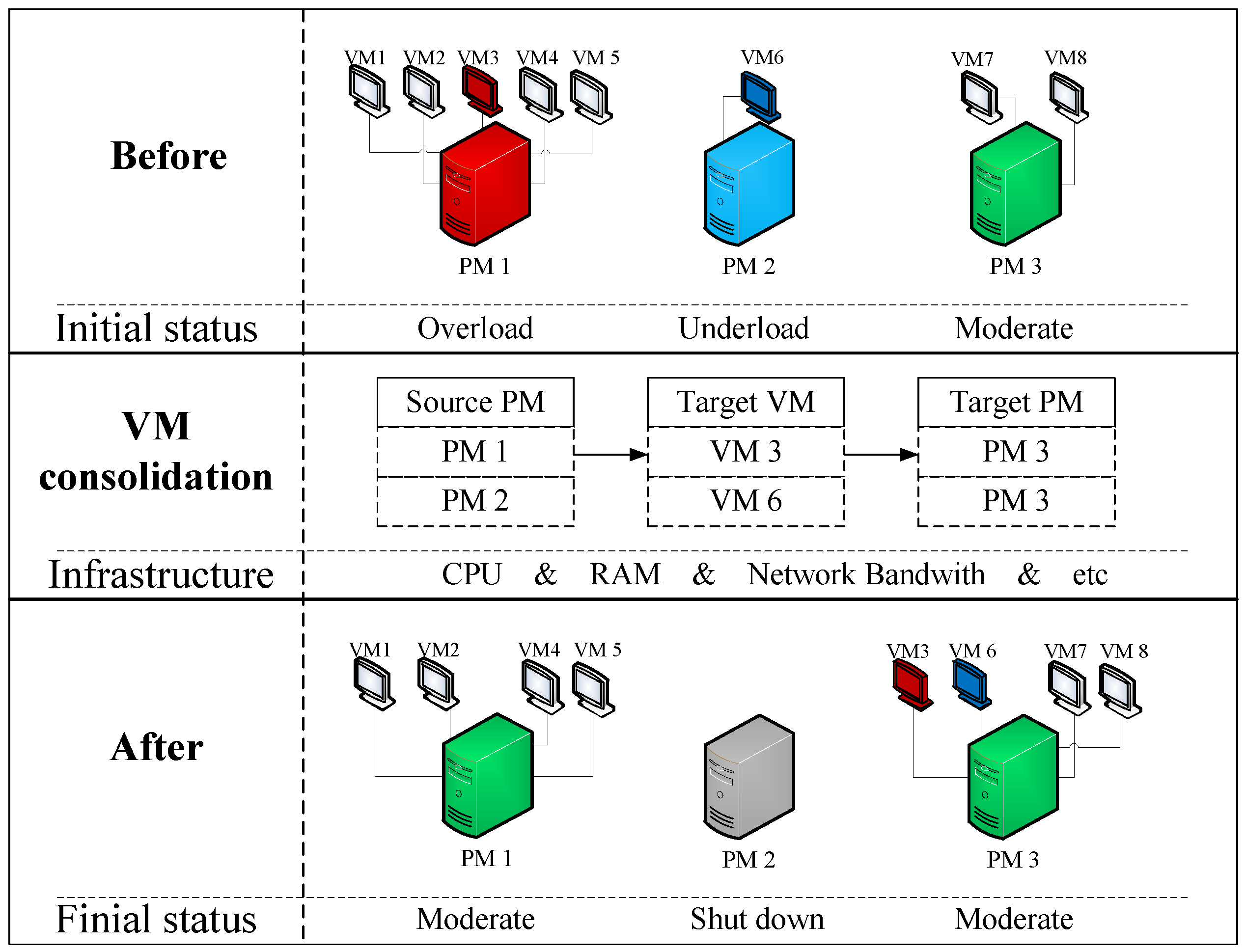
To avoid too much energy consumption caused by the frequent migration of VMs and the low QoS caused by the short shut down during each migration, we decided to prioritize the implementation order of VM consolidation. That is, first migrate some VMs from overload hosts to lower load hosts, and then set all VMs on hosts with low load to migrated out and switch these hosts to sleep mode or shut down.

Thus, DMT has been set to adaptively fit the cloud environment of source PM selection until now, while the parameter of $T_m$ in multi-thresholds will later be taken into consideration in Section 3.2 for helping the selection of target VM during VM consolidation. Once a PM is detected to be overloaded or low load by our defined dynamic multi-thresholds, the next step is to select proper VMs to migrate from this host and we will further discuss the adaptive VM consolidation strategies on the improvement of VM selection and placement based on the dynamic multi-thresholds in Section 3.2 and Section 3.3.

3.2. The Improved MW-MVM Algorithm for VM Selection

To efficiently choose proper target VMs on each selected $Sourc{e}_{PM}$ with fewer VM migrations, [11] first proposed MVM (Minimization of VM Migration) algorithm. The main idea of this method is to sort the CPU utilization of each VM in descending order, and then select the targeted VM to migrated out in two criterions. One of the criterion is that the VM’s CPU utilization should be higher than the difference between the upper threshold and each PM’s present overall CPU utilization. Another criterion is that, compared to values on all VMs, the difference between the new utilization and the upper threshold on each selected VM is the minimum. If there is no suitable VM that satisfied these two criteria, the VM in $Sourc{e}_{PM}$ that has the highest resource utilization will be selected. Unless the new utilization of this source PM is under the upper threshold, all of the above processes will not be repeated any more.

The inadequacy of this method is that it only takes one parameter (CPU utilization) into consideration, while different overload PMs usually have different requests on other resources. Based on that, we try to improve this method within our multi-thresholds by using different weights to efficiently allocate VMs. Below is an example showing the detail of our improved method.

Assume that the current multi-thresholds are $T= \langle T_l, T_u, T_{SLA}, T_m\rangle$, and the load thresholds are $T_l=\langle t_c,t_r,t_b\rangle , T_u=\langle T_c,T_r,T_b\rangle$. The utilization ratio of resource * on $PM\left(j\right)$ can be calculated as

$$P_j^{\ast }=\frac{U_{pmj}^{\ast }}{C_{pmj}^{\ast }}=\frac{{{\displaystyle \sum }}_{i=1}^m{U}_{p_j{v}_i}^{\ast }}{C_{pmj}^{\ast }}$$

(6)

where * represents CPU in $c$, RAM in $r$, Bandwidth in $b$, respectively. Thus, resource utilization ratio on $PM\left(j\right)$ can be expressed as $P_j=\left[ P_j^c, P_j^r, P_j^b \right]$.

We define the formula for the relative difference $Q_j^{\ast }$ between upper threshold and actual utilization of resource * on $PM\left(j\right)$ as

$$Q_j^{\ast }=\{\begin{array}{ll}{P}_j^{\ast }-T_{\ast },& if(P_j^{\ast }>T_{\ast })\\ 0,& else\end{array}$$

(7)

Thus, the relative different of $PM\left(j\right)$ is $Q_j=\left[ Q_j^c, Q_j^r, Q_j^b \right]$, which can then be used as the weights for choosing minimum number VMs since the weights showing the maximize corresponding overload of each resource on $PM\left(j\right)$. The weights of all VMs on $PM\left(j\right)$ can then be calculated as

$$\begin{array}{ll}{W}_{VM}& =U_{p_j{v}_i}^{\ast }·{Q_j}^T\\ & =\left[\begin{array}{ccc}{U}_{p_j{v}_i}^c& U_{p_j{v}_i}^r& U_{p_j{v}_i}^b\end{array}\right]·\left[\begin{array}{c}{Q}_j^c\\ Q_j^r\\ Q_j^b\end{array}\right]\\ & =\left[\begin{array}{c}{W}_{p_j{v}_1}\\ \begin{array}{c}{W}_{p_j{v}_2}\\ ⋮\end{array}\\ W_{p_j{v}_m}\end{array}\right]\end{array}$$

(8)

Here $U_{p_j{v}_i}^{\ast }$ represents the allocated resource in each VM, which indicates the number of various resources that the virtual machine has occupied and $Q_j{}^T$ calculated by (7) shows the difference of each threshold, as the higher value of each resource means the more corresponding of migration requests. Thus, by multiplying $U_{p_j{v}_i}^{\ast }$ and $Q_j{}^T$, the weight of all VMs in $PM\left(j\right)$ can be calculated. For $VM\left(i\right)$ in $PM\left(j\right)$, its weight is represented as $W_{p_j{v}_{\mathrm{i}}}$, which is used to decide the selection of target VM, as well as the number of VMs that need to be migrated out.

To minimize VM migration times, all weights are sorted in descending order. As the higher the weight is, the higher the corresponding request is, the lower the migration times will be. The host ($PM\left(j\right)$) first select the VM with the highest weights and add it to the waiting list, then it will be checked again for being overload (Algorithm 3). If it is still considered as being overloaded, the VM selection policy is applied again to select another VM to migrate from the host. This will be repeated until the host is considered as being not overloaded. The last step is to check the migration number of these selected VMs in the waiting list. If the migration number of some selected VMs has gone over the set threshold $T_m$, it will not be added, otherwise, VMs in the waiting list will be added to $Selec{t}_{VM}$ which contains all VMs that need to be migrated.

Algorithm 3 Improved Multi-weights MVM policy (MW-MVM)

1 Input: $Sourc{e}_{PM}$, $V{M}_{List}$ 2 Output: $Selec{t}_{VM}$ 3 foreach $PM\left(j\right)$ in $Sourc{e}_{PM}$ 4   $Selec{t}_{VM}=\mathrm{NULL}$ 5   calculate $W_{VM}$ using formula (8) 6   order = $W_{VM}$. sortDescendingOrder() 7   foreach $\mathrm{V}M\left(i\right)$ in $PM\left(j\right)$ 8     waitingList ← $\mathrm{V}M\left(i\right)$ with highest value in order 9     $PM\left(j\right)$ ← $PM\left(j\right)-VM\left(i\right)$ 10     update $P_j^{\ast }$ of $PM\left(j\right)$ 11     if (LD ($PM\left(j\right))=0$) then 12       Break 13   foreach $\mathrm{V}M\left(i\right)$ in waitingList 14     if (migration_num($\mathrm{V}M\left(i\right)$ < $T_m$)) then 15       $Selec{t}_{VM}$ ← $\mathrm{V}M\left(i\right)$ 16 if ($Selec{t}_{VM}\ne \mathrm{NULL}$) 17   return $Selec{t}_{VM}$

Without loss of generality, all overload hosts can follow these steps to select the minimum number of VMs. While for low load hosts, all VMs within it will be migrated out and there is no need to execute this VM selection policy before VM allocation and the placement of these selected VMs in the waiting list to which PM is discussed in the next section.

3.3. VM Placement Using Modified MW-BF Algorithm

The VM placement is similar to a bin packing problem on variable bin sizes and prices, where bins represent the physical nodes; items are the VMs that had to be allocated; bin sizes are the available resource capacities (CPU, RAM, Bandwidth, etc.) of the nodes; and prices correspond to the power consumption by the nodes. As the bin packing problem is NP-hard, to solve it we apply a modification of the Best Fit (BF) algorithm by considering the multi-weight of the VM that needs to be allocated. In our modification (MW-BF), we sort all the PMs in the ascending of its resource utilization ratio, multiplied by the weights of the allocating VM. This allocates each VM to a host that provides the least increase of the power consumption and chooses the most power-efficient one by leveraging the heterogeneity of each node.

Use matrix $P^{\ast }$ to represent each resource utilization ratio of all PMs, defined as:

$$P^{\ast }=\left[\begin{array}{c}{P}_1^{\ast }\\ \begin{array}{c}{P}_2^{\ast }\\ ⋮\end{array}\\ P_m^{\ast }\end{array}\right]=\left[\begin{array}{ccc}{P}_1^c& P_1^b& P_1^r\\ \begin{array}{c}{P}_2^c\\ ⋮\end{array}& \begin{array}{c}{P}_2^b\\ ⋮\end{array}& \begin{array}{c}{P}_2^r\\ ⋮\end{array}\\ P_m^c& P_m^b& P_m^r\end{array}\right]$$

(9)

The product of multi-weights and resource utilization of each PM for allocating VM selected from $PM\left(j\right)$ can be calculated as:

$$W_{PM}=P^{\ast }·Q_j{}^T=\left[\begin{array}{ccc}{P}_1^c& P_1^b& P_1^r\\ \begin{array}{c}{P}_2^c\\ ⋮\end{array}& \begin{array}{c}{P}_2^b\\ ⋮\end{array}& \begin{array}{c}{P}_2^r\\ ⋮\end{array}\\ P_m^c& P_m^b& P_m^r\end{array}\right]·\left[\begin{array}{c}{Q}_j^c\\ Q_j^r\\ Q_j^b\end{array}\right]$$

(10)

The pseudo-code for the algorithm is presented in Algorithm 4. The complexity of the algorithm is n·m, where n is the number of nodes and m is the number of VMs that have to be allocated. After these steps, the waiting list $Targe{t}_{PM}$ then contains PMs that need to be migrated in.

Algorithm 4 Modified Multi-weights Best fit (MW-BF)

1 Input: $P{M}_{List}$, $Selec{t}_{VM}$ 2 Output: placement of VMs 3 $Selec{t}_{VM}$. sortDescendingUtilization() 4 foreach VM in $Selec{t}_{VM}$ do 5   calculate each $W_{PM}$ using Formula (10) 6   $W_{PM}$. sortAscendingUtilization() 7   if PM has enough resource for VM then 8     $Targe{t}_{PM}$ ← PM 9     minEnergy ← MAX 10     allocatedPM ← NULL 11     foreach PM in $Targe{t}_{PM}$ do 12       energy ← estimateEnergy (PM, VM) in (13) 13       if energy < minEnergy then 14         allocatedPM ← PM 15         minEnergyr ← energy 16     if allocatedPM $\ne$ NULL then 17         allocate VM to allocatedPM 18 return placement of VMs

The VM first selects the PM with least $W_{PM}$ and adds it to the waiting list ($Targe{t}_{PM}$), then it will be checked for being overload. To maximize the utilization of the remaining resource on these destination PMs, all product $W_{PM}$ are sorted in descending order. In general, the least the product of resource utilization and weights is, the more the corresponding resource it will leave, which means that the VM would have enough remaining resources to use and thus it could efficiently decrease the cost of the frequent migration of VMs.

4. Experiments and Results

4.1. Experiment Setup

It is essential to evaluate the proposed VM consolidation strategy on a large-scale experiment environment with a real infrastructure since the target system is an IaaS Cloud. Yet to conduct repeatable experiments on a real infrastructure is extremely difficult due to the requirements of evaluating and comparing the proposed algorithm. In contrast to alternative simulation toolkits (SimGrid or GangSim), CloudSim [13] allows the modeling of virtualized environments, supporting on-demand resource management and configuration.

Therefore, we choose the CloudSim toolkit 4.0 to simulate our proposed strategy, as it is a modern simulation framework aimed at Cloud computing environments. The experiments selected 50 heterogeneous physical hosts. Each physical node is allocated with 3 to 5 virtual machines initially. When a node is determined as overload or underload compared to our defined dynamic multi-thresholds, the proposed self-adaptive VM consolidation strategy will be triggered. The CPU MIPS (millions instrument per seconds) ratings are equivalent to Amazon EC2 instance types. The users submit requests for provisioning of 200 heterogeneous VMs. Each VM is randomly assigned a workload trace from one of the servers from the workload data. Initially, VMs are allocated according to their parameters assuming 100% utilization. The configuration is shown in

Table 4. Experiment configuration table.

Parameter	Unit	Value
Number of PMs		50
Number of VMs		200
CPU core performance of PMs	MIPS	{2000, 2500, 3000, 4000}
Memory of each PM	G	{1, 2, 4, 8}
Bandwidth of each PM	Mbps	{500, 800, 1000}
CPU core performance of VMs	MIPS	{1000, 1500, 2000, 3000}
Memory of each VM	G	{0.5, 1, 2, 4}
Bandwidth of each VM	Mbps	{100, 200, 400}
initial threshold of $T_l$	< $t_c,t_r,t_b$ >	< 0.3, 0.2, 0.2 >
initial threshold of $T_u$	< $T_c,T_r,T_b$ >	< 0.7, 0.8, 0.8 >
initial threshold of $T_{SLA}$		4%
initial threshold of $T_m$		10

.

Our proposed dynamic multi-thresholds strategy (DMT) is compared with four threshold adjustment strategies. The first strategy uses a static threshold (ST) in which the threshold never changes during the consolidation. The threshold sets to 70% for detecting an over-loaded host and 30% for detecting a low-loaded one. The next two strategies adjust the utilization threshold dynamically based on the statistic method by the median absolute deviation (MAD) and the interquartile range (IQR) while the fourth method (LiRCUP) considers the prediction of CPU utilization on each PM, as it selects the higher one to be the next source PMs instead of adjusting the threshold [14]. Among this strategy, the first three are the benchmark algorithms presented in CloudSim (ST, MAD, IQR) [1] and the last one (LiRCUP) is an improved single-parameter prediction algorithm.

To compare the performance of the proposed dynamic multi-thresholds strategy, the algorithm on VM selection and placement of the above five strategies (ST, MAD, IQR, LiCUP, DMT) are the same, with Minimum VM Migration algorithm (MVM) for VM selection and Best Fit algorithm (BF) for VM placement. For the sixth strategy DMT (MW) in our experiment, its VM selection algorithm is MW-MWM, a modified algorithm of MVM shown in Section 3.2, and its VM placement algorithm is MW-BF shown in Section 3.3. The DMT (MW) strategy is added to further compare the performance with DMT, in terms of the improved VM selection algorithm (MW-MWM) and placement algorithm (MW-BF).

4.2. Evaluation Metrics

• SLA violation

In our experiment, the QoS is defined via SLA violation, as the ratio of unallocated resources demanded by applications and the total requested resources. The unallocated resource can be calculated as the difference between the requested resource ($R_{p_j{v}_i}^{\ast }$) of all VMs and the actual allocated resources ($U_{pmj}^{\ast }$) of all PMs (1). Here * can be represented as CPU, RAM and Bandwidth, respectively and each parameter of this metrics considers the whole life time on each VM.

$$SLA= \frac{{{\displaystyle \sum }}_{j=1}^N{{\displaystyle \int }}_t^T(U_{pmj}^{\ast }\left(t\right)-{{\displaystyle \sum }}_{i=1}^M{R}_{p_j{v}_i}^{\ast })dt}{{{\displaystyle \sum }}_{j=1}^N{{\displaystyle \int }}_t^T{U}_{pmj}^{\ast }\left(t\right)dt}$$

(11)

where M is the number of VMs in $PM\left(j\right)$, N is the number of PMs.

• Energy consumption

Our method will take CPU utilization in priority when considering energy-efficiency, compared to the RAM and Bandwidth. Research on [15] shows that an idle host consumes approximately 70% power of a fully utilized one and the energy costs of each server can be described on both of the power cost and the CPU cost, which can be calculated within a linear relationship. Based on that, we defined our power consumption metrics as follows (2), where $P_{max}$ is set to 250 W and c represents CPU utilization.

$$P\left(c\right)=0.7·P_{max}+0.3·P_{max}·c=P_{max}·\left(0.7+0.3·c\right)$$

(12)

Furthermore, according to each different workload, the changing utilization of CPU can be represented as a function of time: $c\left(t\right)$, Therefore, E in (3) is used to define the total energy consumption by a host.

$$E=\underset{t}{\overset{T}{{\displaystyle \int }}}P\left(c\left(t\right)\right)dt$$

(13)

4.3. Experiment Results and Analysis

The simulations have been run on 10 h of each workload category to determine the algorithm that delivers the best energy consumption, SLA violation and number of VM migrations over different workload types. The optimization algorithms have been run on each iteration of the simulation time. The results are shown in Figure 3 as below:

From the simulation results in Figure 3, we can see that when the entire system is under low workload or high workload, our proposed algorithm is superior to the other four algorithms in energy consumption, SLA violation rate, and VM migrations. When the overall system load is medium workload, the consumption of energy and VM migrations of this algorithm are not much different from that of other algorithms, but the rate of SLA violation is obviously lower.

In terms of energy saving, when the system is under a low workload, the DMT strategy improves the energy saving on about 41.9% (3.1 KWh) over the MAD algorithm and improves 25.8% (4.5 KWh) over the LiRCUP when the system is at a high load. For SLA violation rate, when the system is at a high load, DMT algorithm and DMT (MW) algorithm both effectively reduce the violation rate of the overall system in almost 2%. While for VM migration costs, the strategy of this article results in fewer VM migrations, and the DMT (MW) strategy further reduces the number of virtual machine migrations and thus reduces migration costs.

Figure 4 shows the number of active hosts at each moment (that is, the number of PMs that still service VM tasks). When VMs are consolidated by using different strategies, the original hosts with low loads will migrate out of all VMs they own and will be set to sleep mode or shutdown. Thus, counting the current number of active hosts can effectively reflect the effectiveness of the VM consolidation strategy.

It can be clearly seen from Figure 4 that when the whole system is under low workload (a), our proposed VM consolidation strategy can shut down a larger number of hosts and can reach a steady state faster than any other strategies within less than 5 h; when the system workload is moderate (b), the number of shut-down hosts among these six strategies is not much different, with LiRCUP having the lowest number of active hosts; when the overall system is at high load (c), all these algorithms can only shut down a few hosts. Although our proposed algorithm cannot reach a stable state quickly in this situation, it still has the least number of active hosts, which effectively reduces the energy consumption of the system.

Therefore, our proposed VM consolidation strategy based on DMT has more obvious advantages in case of high workload and low workload, especially when it is combined with MW-MVM and MW-BF algorithm on MW-DMT. This result is also consistent with the conclusion in Figure 1, which further demonstrates the superiority of our proposed VM consolidation strategy based on the dynamic multi-thresholds.

5. Related Work

Virtual machine consolidation [6] is one of the techniques in a cloud resource management system to increase the energy-efficiency of IaaS Cloud, since the failure of existing PMs or the addition of new PMs are continuous events happening in cloud data centers. Nathuji and Schwan [16] first proposed an architecture of energy management system for virtualized data centers where resource management is divided into local and global policies. Srikantaiah et al. [17] then proposed a heuristic method to handle the optimization over multiple resources, as they considered the VM consolidation as a bin packing problem. Cardosa et al. [18] have leveraged the min, max and shares parameters of Xen’s VMM to represent minimum, maximum and proportion of the CPU allocated to VMs sharing the same resource.

Threshold-based VM consolidation strategy use upper and lower threshold values to identify a PM as overloaded or underloaded, respectively. Secron [19] considers an upper threshold to prevent PM from reaching 100% utilization with performance degradation. To select the proper PMs for consolidation, Feller et al. [10] propose a static CPU threshold to detect under-loaded and over-loaded PMs. However, although setting static thresholds is simple and appealing, it is not efficient for an environment with dynamic workloads, since different types of application may be running on one single PM. Therefore, threshold values should be adjusted to each workload type and level, which will help optimize the performance VM consolidation efficiently.

To dynamically consolidate the virtual machines in the procedure of selecting source PM, Beloglazov [1] proposed adaptive upper and lower thresholds based on the statistical analysis of the historical data while Farahnakian [14] propose a regression-based prediction model to forecast resource utilization of both PMs and VMs. Recent research on adaptive threshold-based dynamic VM consolidation algorithms [20,21] is using a similar solution, in which the threshold value adapts with the change of different resource utilization. However, the above methods only consider single-resource utilization of the infrastructure, yet do not consider other corresponding sources.

To try to consider other multiple resources, Lu Liu [22] researched the load balance of each application among different virtual machines, but he did not consider the placement of each VM. The research of Xu Jing [23] is consistent with ours; they use multi-resource to optimize the placement of virtual machine but in order to realize the goals of the performance on power and temperature, they do not focus on the study of thresholds as it gives only two sets of thresholds of each parameter, but each threshold is set in static value. In general, although the above researches all consider multi-resources, they do not focus on the optimization of threshold-based VM consolidation in the step for PM selection.

While in the second step of VM consolidation of VM selection, different algorithms are proposed. VMs that have the highest correlation of the resource utilization with other VMs are selected, which is called MC algorithm [4]. Another algorithm called MVM proposed in [24] shows that, it first sorts the VMs in descending order with respect to CPU demand and then selects the VM that satisfies the two author-defined criterions. HPG algorithm was also discussed by the same author, that is selecting the VM with lowest ratio of actual resource usage to its initial claimed resource demand. The VM which requires minimum time to complete the migration is selected for migration called MMT in [1], while the migration time is estimated as the amount of RAM utilized by a VM divided by the spare network bandwidth available for the PM.

However, apart from MMT, the rest of the VM selection algorithms only consider CPU demand of VMs but ignore the memory or network bandwidth requirement of VMs. As argued by [11], selecting a VM only based on CPU will cause saturation in terms of CPU and can lead towards no further improvement in utilization while leaving other types of resources underutilized. It is highly challenging to determine a single converging point representing the equivalent total resource demand of a multitude of resource types, while different types of resources represent different dimensions [9].

6. Conclusions and Future Work

In this paper, we present a novel self-adaptive VM consolidation strategy based on dynamic multi-thresholds (DMT) in IaaS Clouds. First, we define each parameter of the multi-thresholds, including CPU, RAM, Bandwidth, SLA, VM migrations, as well as a dynamic adjustment mechanism for these parameters of the threshold. After that, we improve the VM selection algorithm (MW-MVM) based on this dynamic multi-threshold, which fully utilizes the multi-dimensional parameters of our proposed dynamic threshold by predicting their future values. To further reduce the cost of VM migration and improve the efficiency of VM consolidation, a modified VM placement algorithm is then discussed (MW-BF). Finally, the experiments of the proposed strategy are performed on CloudSim, compared with the three benchmark strategies and one prediction strategy. The simulation results show that our proposed dynamic multi-thresholds strategy (DMT and DMT (MW)) for VM migration has a good performance, not only in lower SLA violation, but also in less energy cost and VM migrations. Particularly, these advantages of our proposed VM consolidation strategy are much superior than other strategies when the whole cloud system is at high or low workload, as well as the reduction in number of active hosts.

Furthermore, since the experimental objects in this paper are only 50 heterogeneous servers, the number of PMs in the real cloud system is often as high as the tens of thousands. Thus, the effect of energy-efficiency and QoS for VM consideration using our proposed strategy will be much more obvious, which will help further decrease carbon dioxide and overall energy consumption in IaaS clouds. In the future, we plan to consider other different parameters in the multi-thresholds strategy and will further explore the impact weights of each parameter. At the same time, we will also focus on the modification of other VM selection and placement algorithms to further improve the migration-efficiency and energy-efficiency of VM consolidation in IaaS clouds.