

Accelerating Biologics PBPK Modelling with Automated Model Building: A Tutorial

 , ,
, ,
Abstract
1. Introduction
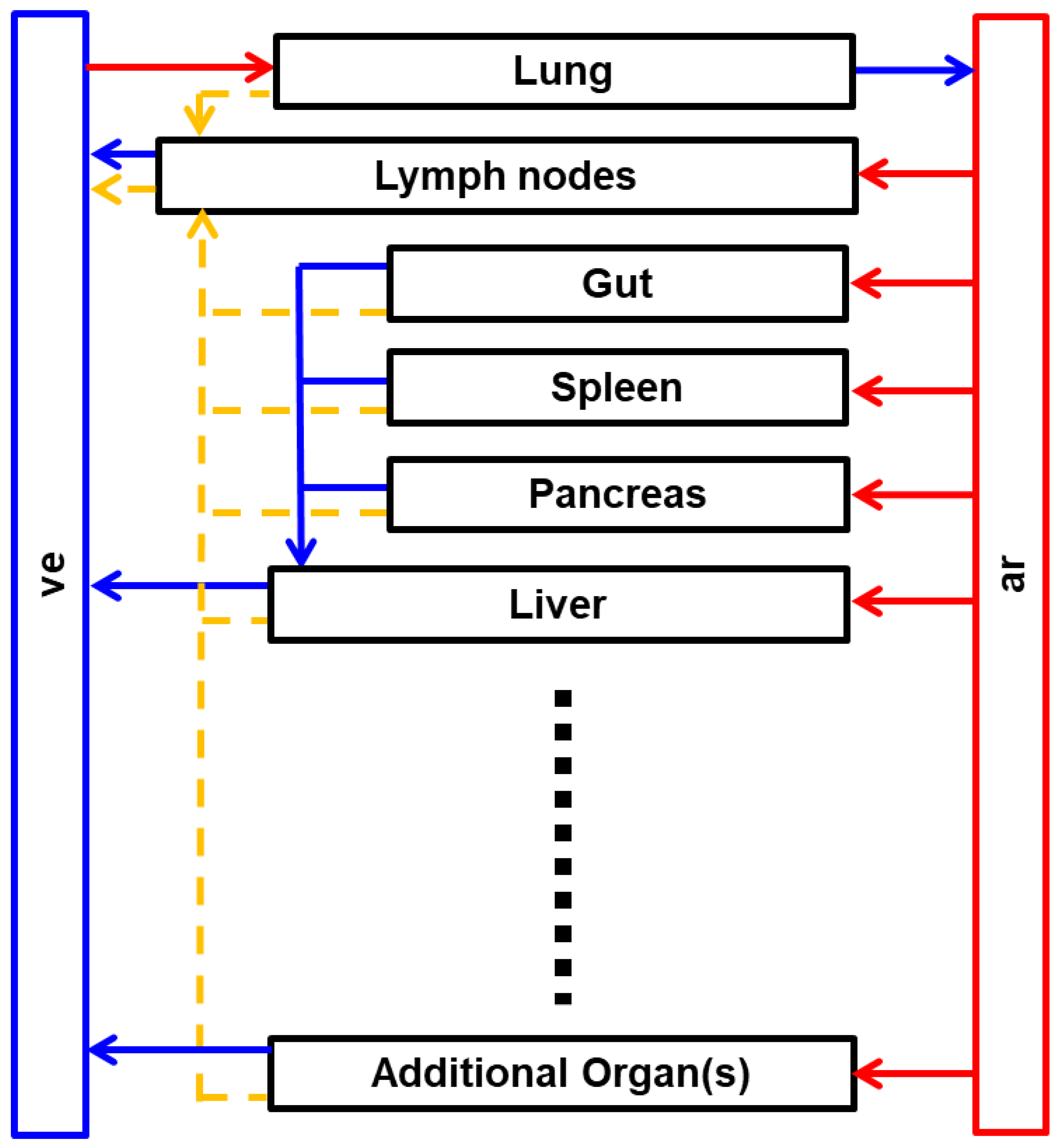
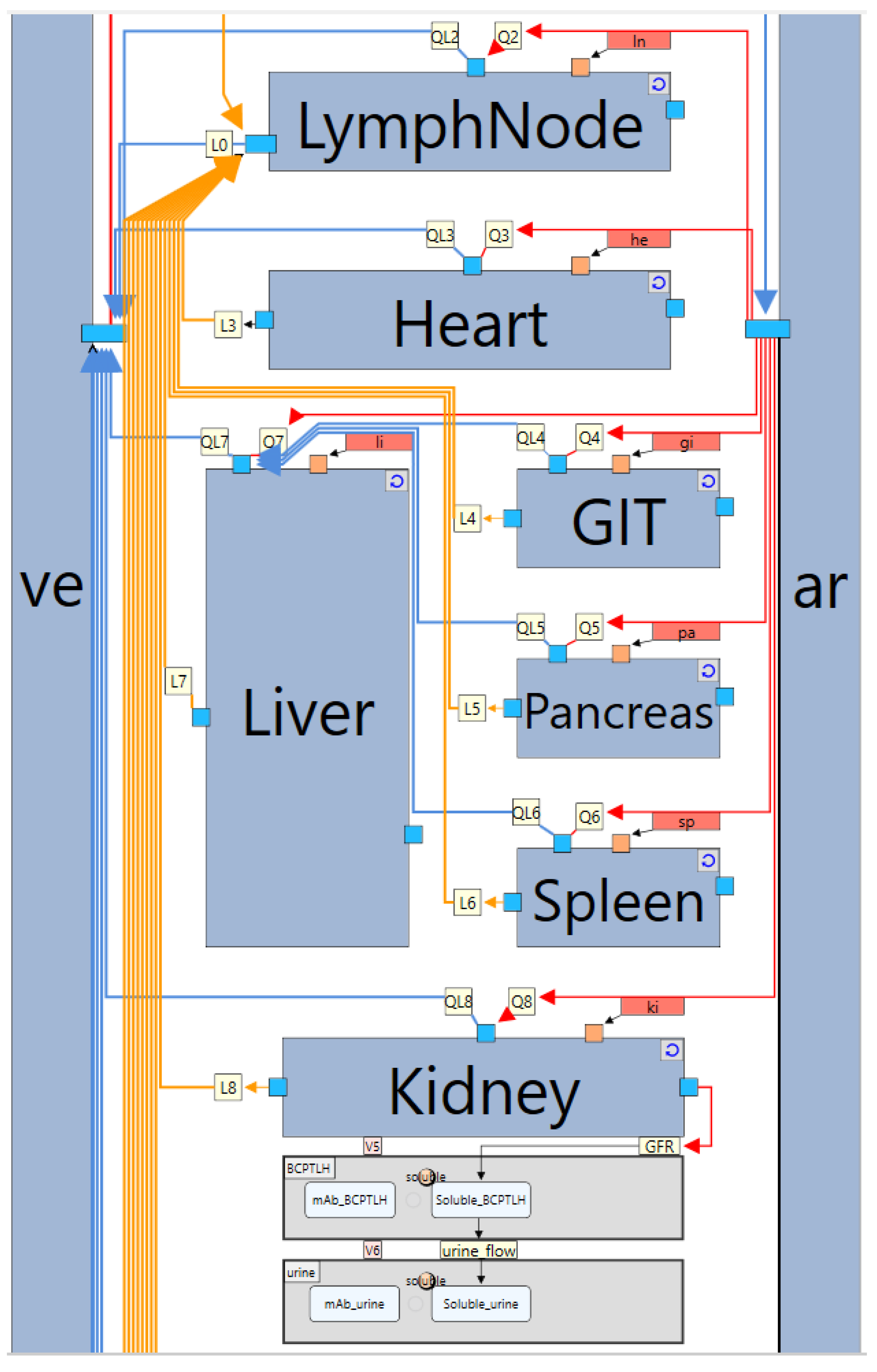
2. Whole-Body PBPK Model Structure
3. Mechanistic Determinants of Biologics Disposition
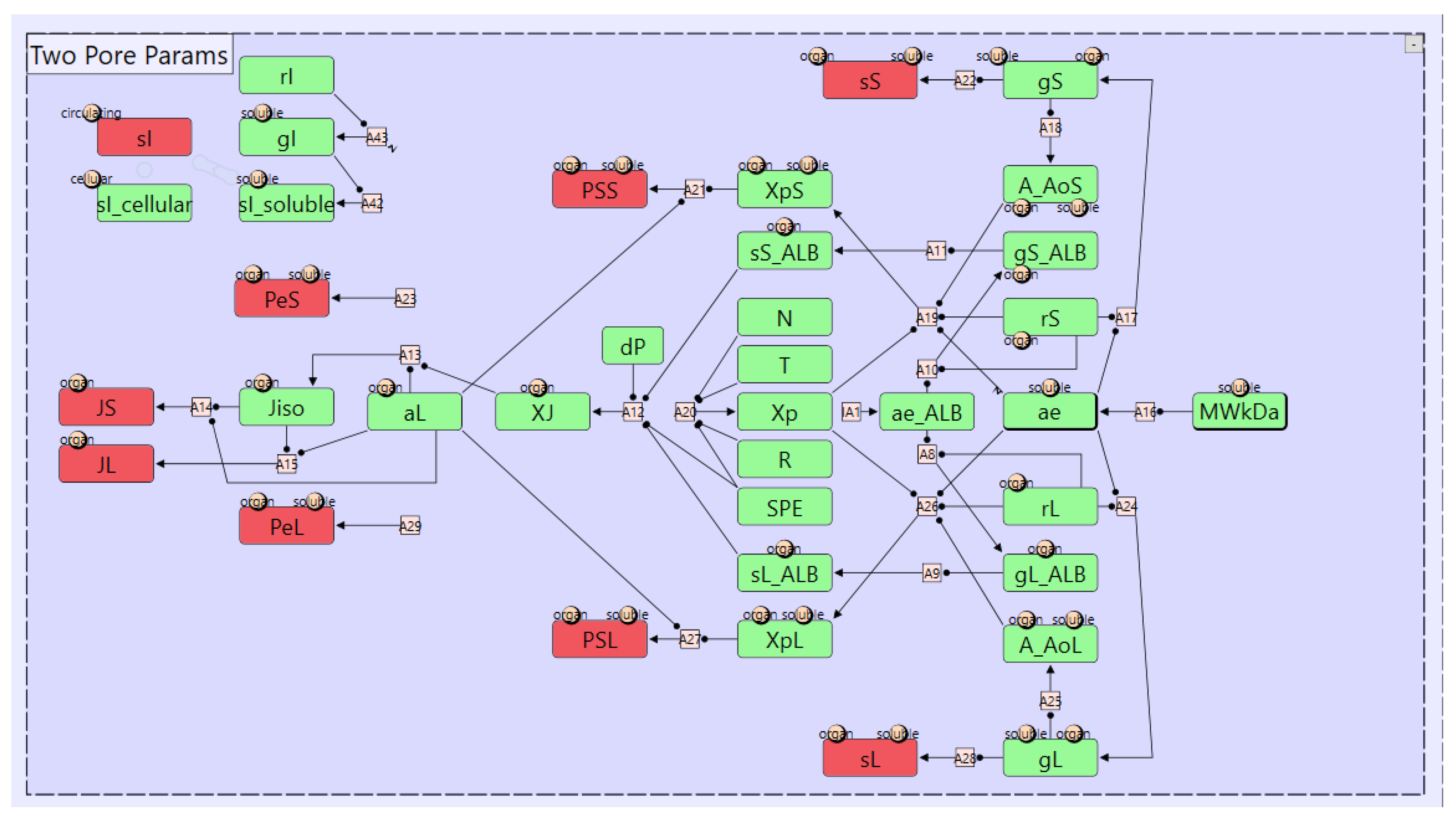
3.1. Two-Pore Formalism for Transcapillary Transport
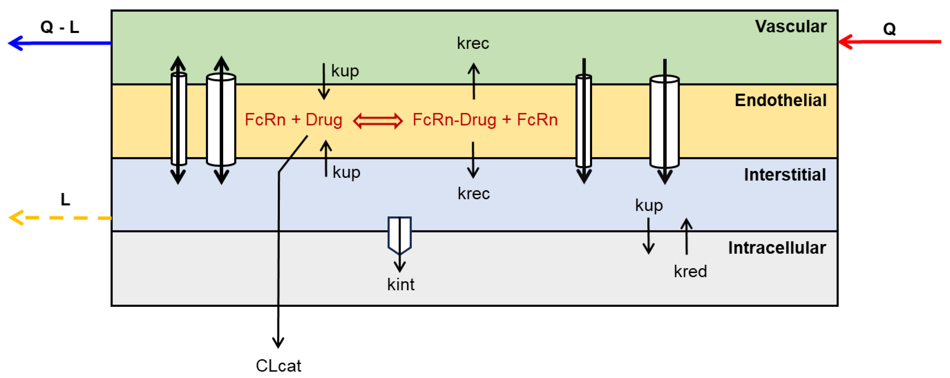
3.2. Catabolic Clearance and FcRn-Mediated Recylcing and Transcytosis
3.3. Renal Elimination
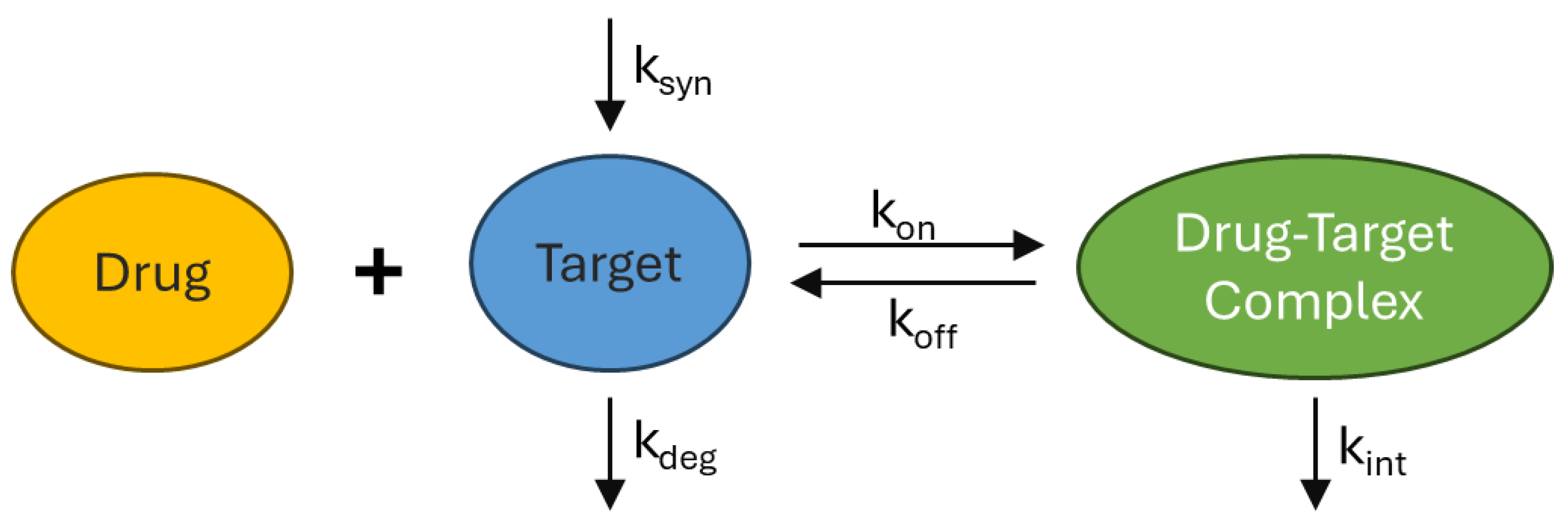
3.4. Target Mediated Drug Disposition & Receptor Mediated Endocytosis
4. Introduction to Simcyp Designer
- (a)
- “Species” nodes, which represent dynamic states in the ODE model. Note that the term “Species” here refers to mathematical states, not biological species. When referring to different biological species, we explicitly use “animal species”, and
- (b)
- “Parameter” nodes, which define parameters in the ODE model.
- (a)
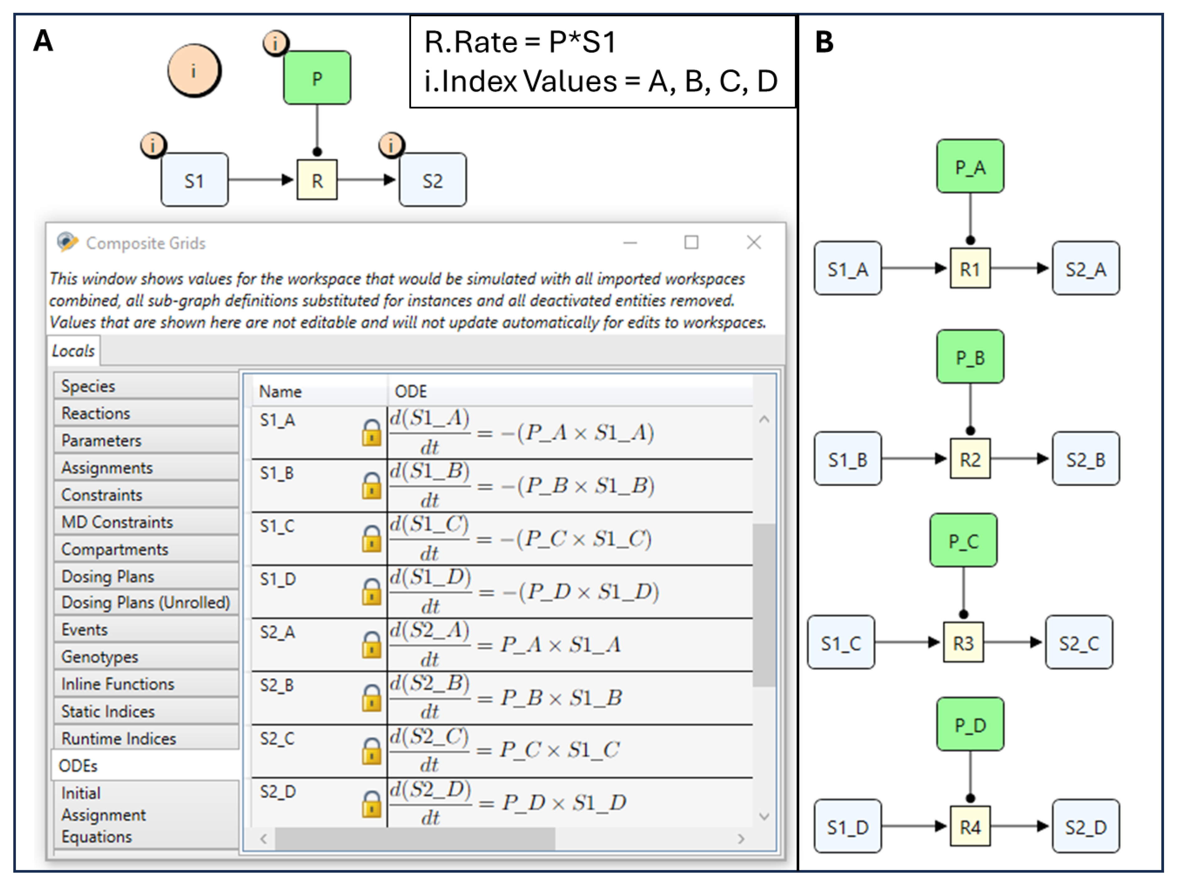
- “Reaction” nodes, which consume and produce “Species”, i.e., represent ODE terms,
- (b)
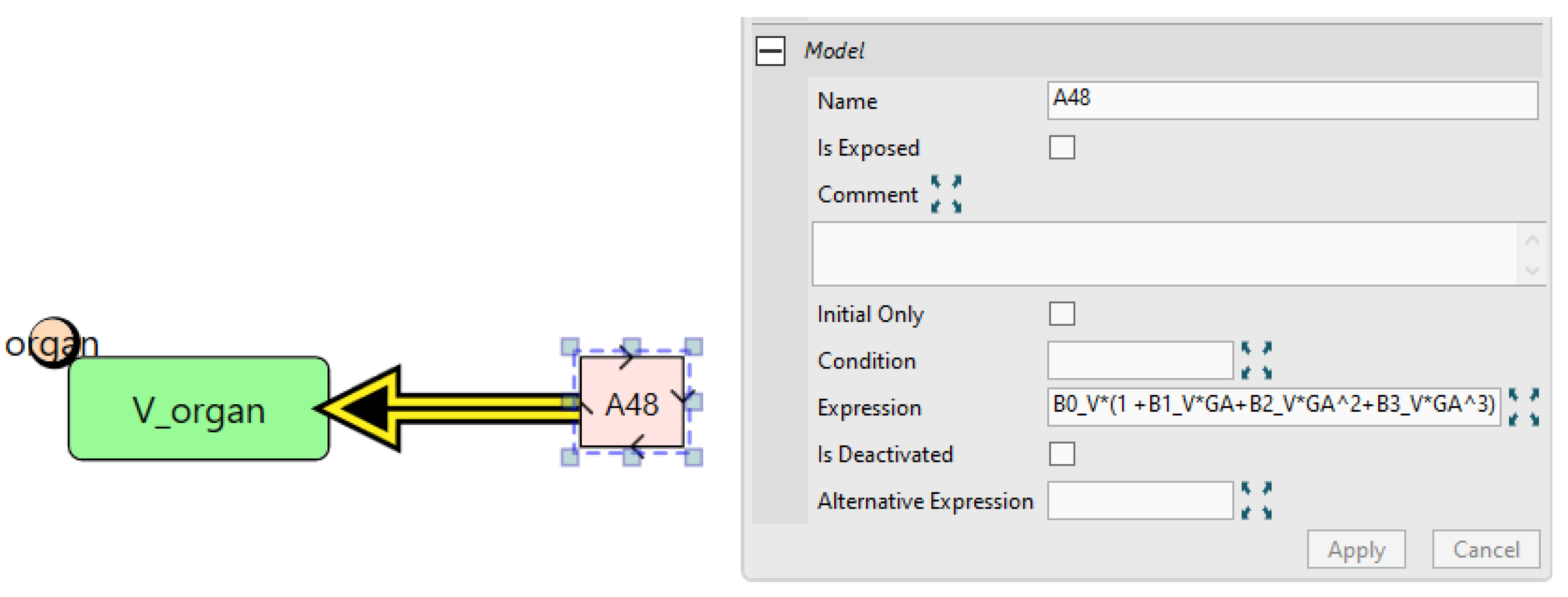
- “Assignment” nodes, which assign values to quantity nodes based on evaluated expressions. These can be either repeated assignments for time-varying quantities or initial assignments for fixed quantities.
- (c)
- “Dosing Plan” nodes, which specify times and amounts (or rates) of doses to “Species”.
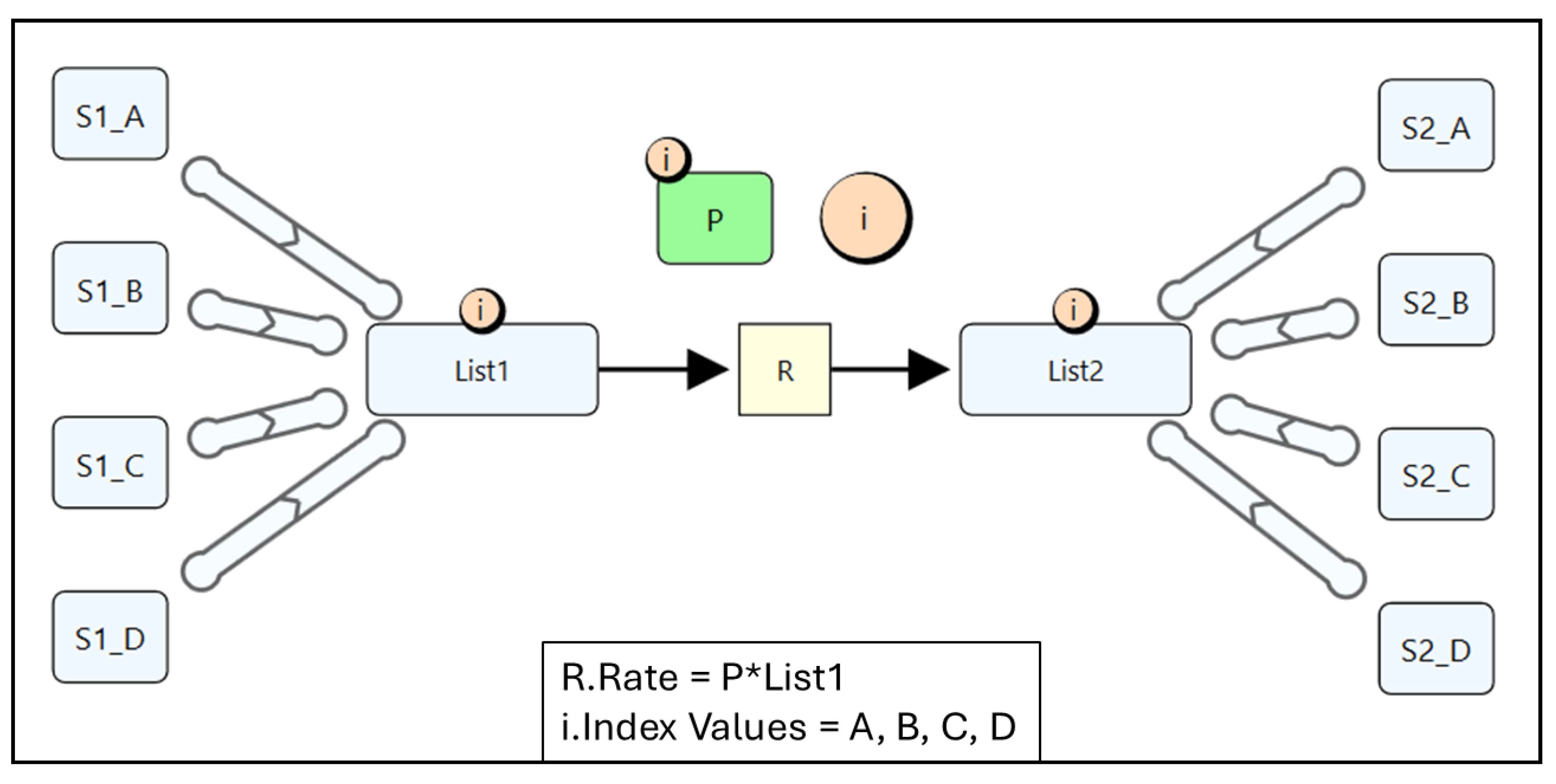
4.1. Quantity Arrays
4.2. Reusable Subgraphs
4.3. Quantity Lists
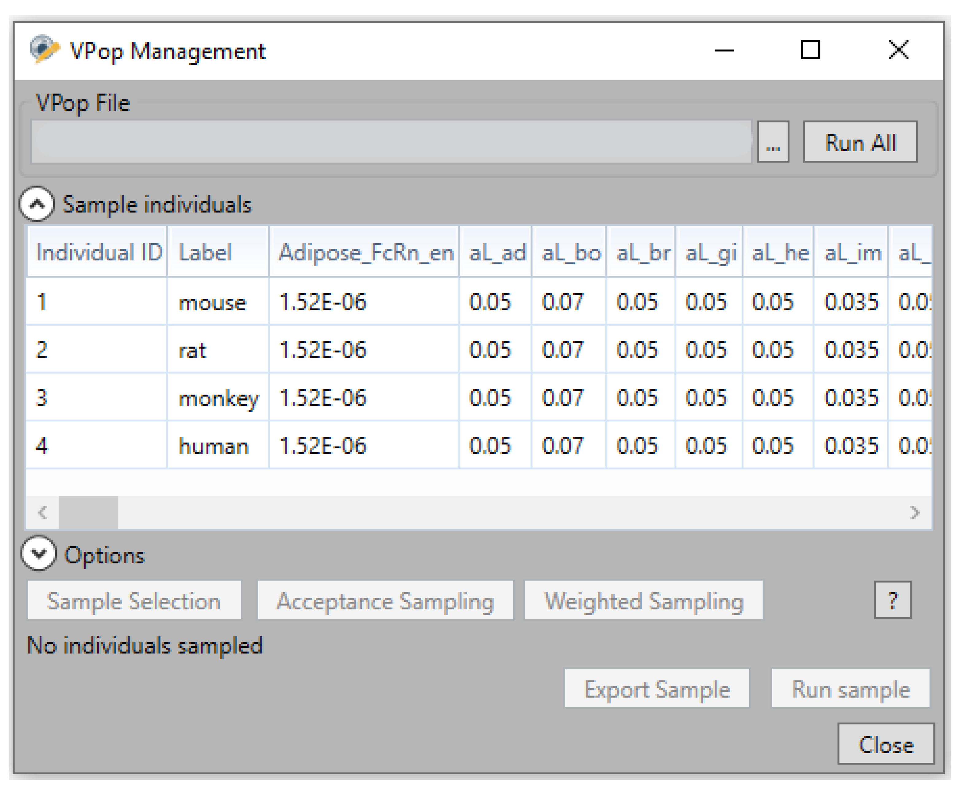
4.4. Virtual Population (VPop) Files
5. Application Case Studies
5.1. Case Study 1: A Model for Monoclonal Antibodies
- Indices
- 2.
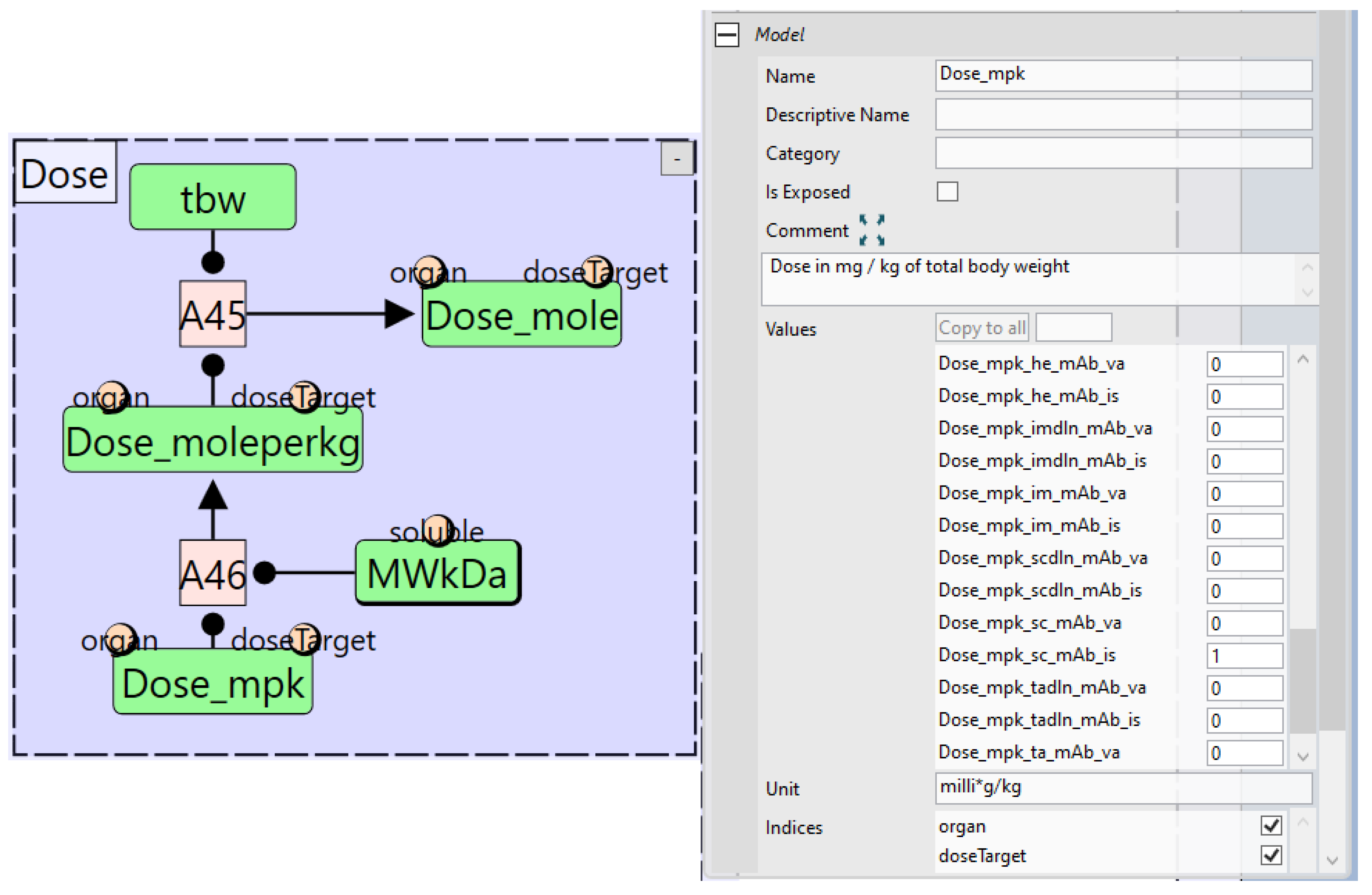
- Parameters Module
- 3.
- Organ-level subgraph definition
- Index value node
- b.
- Compartments
- c.
- Dosing Plan
- d.
- Species and Species Lists
- e.
- Reactions
- 4.
- Whole-body level module
- 5.
- Cross-species simulations
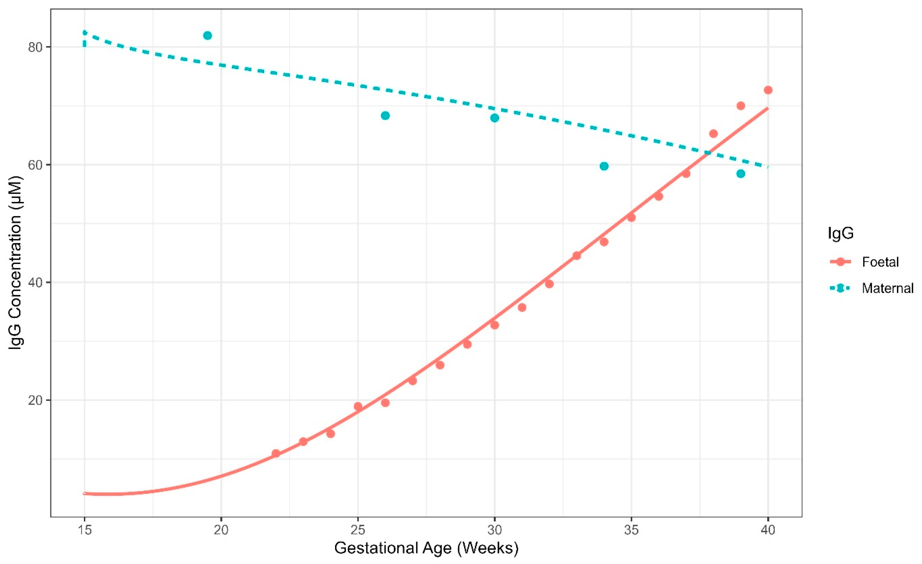
5.2. Case Study 2: Pregnancy IgG Model
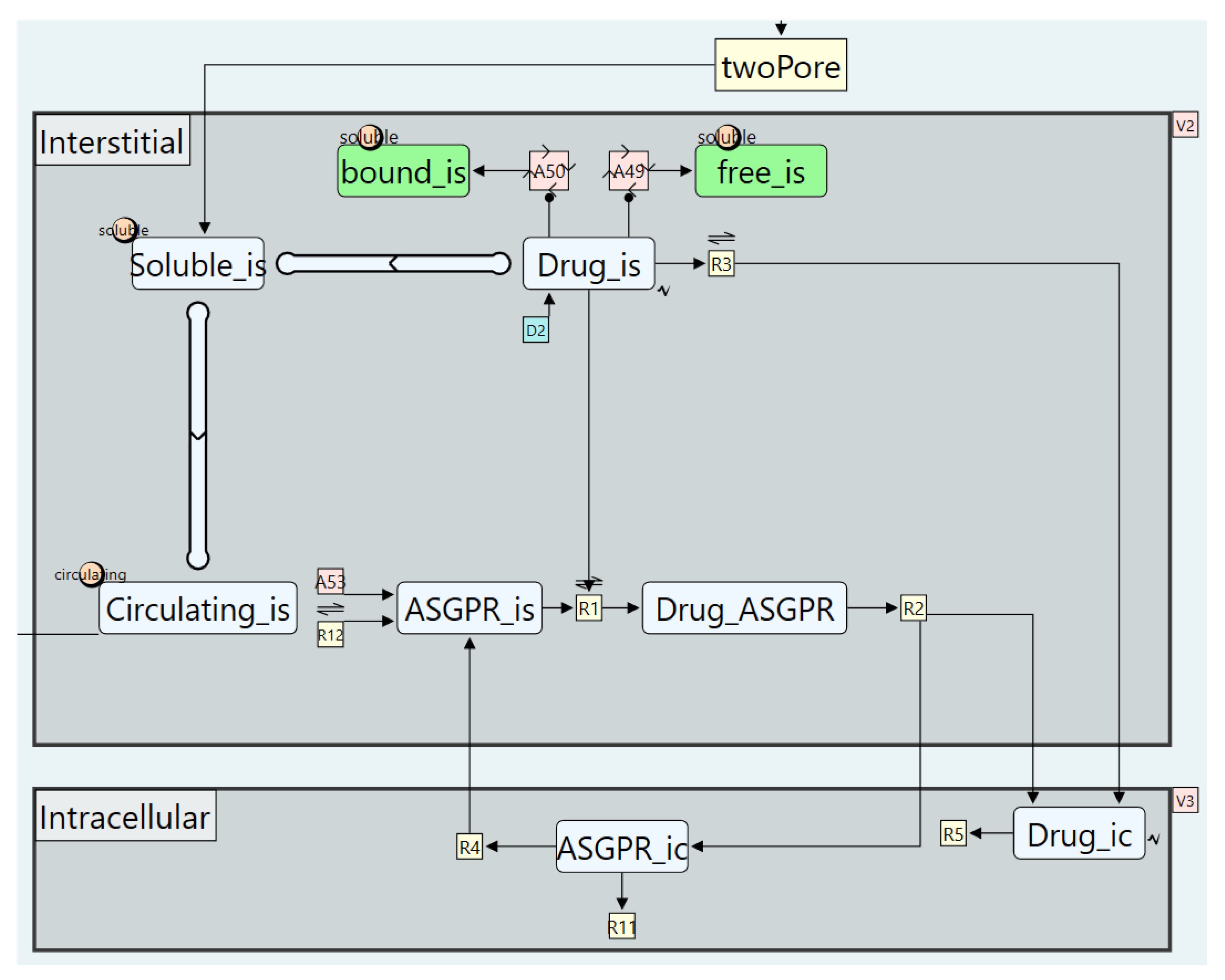
5.3. Case Study 3: A Targeted Oligonucleotides Model
- Modelling Plasma Protein Binding
- 2.
- Disabling the FcRn recycling pathway
- 3.
- Modelling intracellular uptake
- 4.
- VPop simulations
6. Discussion and Conclusions
Supplementary Materials
Author Contributions
Funding
Acknowledgments
Conflicts of Interest
References
- Leader, B.; Baca, Q.J.; Golan, D.E. Protein therapeutics: A summary and pharmacological classification. Nat. Rev. Drug Discov. 2008, 7, 21–39. [Google Scholar] [CrossRef] [PubMed]
- Zhao, L.; Ren, T.H.; Wang, D.D. Clinical pharmacology considerations in biologics development. Acta Pharmacol. Sin. 2012, 33, 1339–1347. [Google Scholar] [CrossRef] [PubMed]
- Jones, H.; Chen, Y.; Gibson, C.; Heimbach, T.; Parrott, N.; Peters, S.; Snoeys, J.; Upreti, V.; Zheng, M.; Hall, S. Physiologically based pharmacokinetic modeling in drug discovery and development: A pharmaceutical industry perspective. Clin. Pharmacol. Ther. 2015, 97, 247–262. [Google Scholar] [CrossRef]
- Gieschke, R.; Steimer, J.L. Pharmacometrics: Modelling and simulation tools to improve decision making in clinical drug development. Eur. J. Drug Metab. Pharmacokinet. 2000, 25, 49–58. [Google Scholar] [CrossRef] [PubMed]
- Lippert, J.; Brosch, M.; von Kampen, O.; Meyer, M.; Siegmund, H.-U.; Schafmayer, C.; Becker, T.; Laffert, B.; Görlitz, L.; Schreiber, S.; et al. A Mechanistic, Model-Based Approach to Safety Assessment in Clinical Development. CPT: Pharmacomet. Syst. Pharmacol. 2012, 1, 13. [Google Scholar] [CrossRef]
- Zhao, P.; Zhang, L.; Grillo, J.; Liu, Q.; Bullock, J.; Moon, Y.; Song, P.; Brar, S.; Madabushi, R.; Wu, T.; et al. Applications of Physiologically Based Pharmacokinetic (PBPK) Modeling and Simulation During Regulatory Review. Clin. Pharmacol. Ther. 2011, 89, 259–267. [Google Scholar] [CrossRef]
- Glassman, P.M.; Balthasar, J.P. Mechanistic considerations for the use of monoclonal antibodies for cancer therapy. Cancer Biol. Med. 2014, 11, 20–33. [Google Scholar] [CrossRef]
- Derbalah, A.; Jamei, M.; Gardner, I.; Sepp, A. The role of automation in enhancing reproducibility and interoperability of PBPK models. Brief. Bioinform. 2025, 26, bbaf053. [Google Scholar] [CrossRef]
- Matthews, R.J.; Hollinshead, D.; Morrison, D.; van der Graaf, P.H.; Kierzek, A.M. QSP Designer: Quantitative systems pharmacology modeling with modular biological process map notation and multiple language code generation. CPT Pharmacomet. Syst. Pharmacol. 2023, 12, 889–903. [Google Scholar] [CrossRef]
- Jones, H.; Rowland-Yeo, K. Basic Concepts in Physiologically Based Pharmacokinetic Modeling in Drug Discovery and Development. CPT Pharmacomet. Syst. Pharmacol. 2013, 2, 63. [Google Scholar] [CrossRef]
- Liu, S.; Li, Y.; Li, Z.; Wu, S.; Harrold, J.M.; Shah, D.K. Translational two-pore PBPK model to characterize whole-body disposition of different-size endogenous and exogenous proteins. J. Pharmacokinet. Pharmacodyn. 2024, 51, 449–476. [Google Scholar] [CrossRef] [PubMed]
- Baxter, L.T.; Zhu, H.; Mackensen, D.G.; Jain, R.K. Physiologically based pharmacokinetic model for specific and nonspecific monoclonal antibodies and fragments in normal tissues and human tumor xenografts in nude mice. Cancer Res. 1994, 54, 1517–1528. [Google Scholar]
- Cao, Y.; Jusko, W.J. Applications of minimal physiologically-based pharmacokinetic models. J. Pharmacokinet. Pharmacodyn. 2012, 39, 711–723. [Google Scholar] [CrossRef]
- Grotte, G. Passage of dextran molecules across the blood-lymph barrier. Acta Chir. Scand. Suppl. 1956, 211, 1–84. [Google Scholar] [PubMed]
- Rippe, B.; Haraldsson, B. Fluid and protein fluxes across small and large pores in the microvasculature. Application of two-pore equations. Acta Physiol. Scand. 1987, 131, 411–428. [Google Scholar] [CrossRef]
- Sepp, A.; Meno-Tetang, G.; Weber, A.; Sanderson, A.; Schon, O.; Berges, A. Computer-assembled cross-species/cross-modalities two-pore physiologically based pharmacokinetic model for biologics in mice and rats. J. Pharmacokinet. Pharmacodyn. 2019, 46, 339–359. [Google Scholar] [CrossRef] [PubMed]
- Sepp, A.; Berges, A.; Sanderson, A.; Meno-Tetang, G. Development of a physiologically based pharmacokinetic model for a domain antibody in mice using the two-pore theory. J. Pharmacokinet. Pharmacodyn. 2015, 42, 97–109. [Google Scholar] [CrossRef]
- Pyzik, M.; Rath, T.; Lencer, W.I.; Baker, K.; Blumberg, R.S. FcRn: The Architect Behind the Immune and Nonimmune Functions of IgG and Albumin. J. Immunol. 2015, 194, 4595–4603. [Google Scholar] [CrossRef]
- Tzaban, S.; Massol, R.H.; Yen, E.; Hamman, W.; Frank, S.R.; Lapierre, L.A.; Hansen, S.H.; Goldenring, J.R.; Blumberg, R.S.; Lencer, W.I. The recycling and transcytotic pathways for IgG transport by FcRn are distinct and display an inherent polarity. J. Cell Biol. 2009, 185, 673–684. [Google Scholar] [CrossRef]
- Haraldsson, B.; Nyström, J.; Deen, W.M. Properties of the Glomerular Barrier and Mechanisms of Proteinuria. Physiol. Rev. 2008, 88, 451–487. [Google Scholar] [CrossRef]
- Muliaditan, M.; Sepp, A. Application of quantitative protein mass spectrometric data in the early predictive analysis of target engagement by monoclonal antibodies. Clin. Transl. Sci. 2022, 15, 1634–1643. [Google Scholar] [CrossRef] [PubMed]
- Meibohm, B.; Zhou, H. Characterizing the Impact of Renal Impairment on the Clinical Pharmacology of Biologics. J. Clin. Pharmacol. 2012, 52, 54S–62S. [Google Scholar] [CrossRef] [PubMed]
- Dua, P.; Hawkins, E.; van der Graaf, P. A Tutorial on Target-Mediated Drug Disposition (TMDD) Models. CPT: Pharmacomet. Syst. Pharmacol. 2015, 4, 324–337. [Google Scholar] [CrossRef] [PubMed]
- Stein, A.M.; Peletier, L.A. Predicting the Onset of Nonlinear Pharmacokinetics. CPT: Pharmacomet. Syst. Pharmacol. 2018, 7, 670–677. [Google Scholar] [CrossRef]
- Mager, D.E.; Jusko, W.J. General Pharmacokinetic Model for Drugs Exhibiting Target-Mediated Drug Disposition. J. Pharmacokinet. Pharmacodyn. 2001, 28, 507–532. [Google Scholar] [CrossRef]
- Sepp, A.; Muliaditan, M. Application of quantitative protein mass spectrometric data in the early predictive analysis of membrane-bound target engagement by monoclonal antibodies. mAbs 2024, 16, 2324485. [Google Scholar] [CrossRef]
- Kaufman, R.J.; Popolo, L. Chapter 5—Protein Synthesis, Processing, and Trafficking. In Hematology (Seventh Edition); Hoffman, R., Benz, E.J., Silberstein, L.E., Heslop, H.E., Weitz, J.I., Anastasi, J., Salama, M.E., Abutalib, S.A., Eds.; Elsevier: Amsterdam, The Netherlands, 2018; pp. 45–58.e41. [Google Scholar]
- Byun, J.H.; Park, A.; Jung, I.H. Receptor-mediated endocytosis modeling of antibody-drug conjugates to the released payload within the intracellular space considering target antigen expression levels. J. Appl. Anal. Comput. 2020, 10, 1848–1868. [Google Scholar] [CrossRef]
- Tyagi, P.; Harper, G.; McGeehan, P.; Davis, S.P. Current status and prospect for future advancements of long-acting antibody formulations. Expert. Opin. Drug Deliv. 2023, 20, 895–903. [Google Scholar] [CrossRef]
- Shah, D.K.; Betts, A.M. Towards a platform PBPK model to characterize the plasma and tissue disposition of monoclonal antibodies in preclinical species and human. J. Pharmacokinet. Pharmacodyn. 2012, 39, 67–86. [Google Scholar] [CrossRef]
- Keizer, R.J.; Huitema, A.D.R.; Schellens, J.H.M.; Beijnen, J.H. Clinical Pharmacokinetics of Therapeutic Monoclonal Antibodies. Clin. Pharmacokinet. 2010, 49, 493–507. [Google Scholar] [CrossRef]
- Gill, K.L.; Machavaram, K.K.; Rose, R.H.; Chetty, M. Potential Sources of Inter-Subject Variability in Monoclonal Antibody Pharmacokinetics. Clin. Pharmacokinet. 2016, 55, 789–805. [Google Scholar] [CrossRef] [PubMed]
- Isoherranen, N. Physiologically based pharmacokinetic modeling of small molecules: How much progress have we made? Drug Metab. Dispos. 2025, 53, 100013. [Google Scholar] [CrossRef]
- Gill, K.L.; Jones, H.M. Opportunities and Challenges for PBPK Model of mAbs in Paediatrics and Pregnancy. AAPS J. 2022, 24, 72. [Google Scholar] [CrossRef] [PubMed]
- Sarvas, H.; Seppälä, I.; Kurikka, S.; Siegberg, R.; Mäkelä, O. Half-life of the maternal IgG1 allotype in infants. J. Clin. Immunol. 1993, 13, 145–151. [Google Scholar] [CrossRef]
- Malek, A.; Sager, R.; Kuhn, P.; Nicolaides, K.H.; Schneider, H. Evolution of Maternofetal Transport of Immunoglobulins During Human Pregnancy. Am. J. Reprod. Immunol. 1996, 36, 248–255. [Google Scholar] [CrossRef]
- Ikuta, T.; Iwatani, S.; Yoshimoto, S. Determination and verification of reference intervals of serum immunoglobulin G at birth. Ann. Clin. Biochem. 2024, 61, 319–326. [Google Scholar] [CrossRef] [PubMed]
- Watts, J.K.; Corey, D.R. Silencing disease genes in the laboratory and the clinic. J. Pathol. 2012, 226, 365–379. [Google Scholar] [CrossRef]
- Chen, P.; Wei, Y.; Sun, T.; Lin, J.; Zhang, K. Enabling safer, more potent oligonucleotide therapeutics with bottlebrush polymer conjugates. J. Control. Release 2024, 366, 44–51. [Google Scholar] [CrossRef]
- Nair, J.K.; Willoughby, J.L.S.; Chan, A.; Charisse, K.; Alam, M.R.; Wang, Q.; Hoekstra, M.; Kandasamy, P.; Kel’in, A.V.; Milstein, S.; et al. Multivalent N-Acetylgalactosamine-Conjugated siRNA Localizes in Hepatocytes and Elicits Robust RNAi-Mediated Gene Silencing. J. Am. Chem. Soc. 2014, 136, 16958–16961. [Google Scholar] [CrossRef]
- Matsuda, S.; Keiser, K.; Nair, J.K.; Charisse, K.; Manoharan, R.M.; Kretschmer, P.; Peng, C.G.; Kel’in, A.V.; Kandasamy, P.; Willoughby, J.L.S.; et al. siRNA Conjugates Carrying Sequentially Assembled Trivalent N-Acetylgalactosamine Linked Through Nucleosides Elicit Robust Gene Silencing In Vivo in Hepatocytes. ACS Chem. Biol. 2015, 10, 1181–1187. [Google Scholar] [CrossRef]
- Zhang, R.; Diasio, R.B.; Lu, Z.; Liu, T.; Jiang, Z.; Galbraith, W.M.; Agrawal, S. Pharmacokinetics and tissue distribution in rats of an oligodeoxynucleotide phosphorothioate (GEM 91) developed as a therapeutic agent for human immunodeficiency virus type-1. Biochem. Pharmacol. 1995, 49, 929–939. [Google Scholar] [CrossRef] [PubMed]
- Nair, J.K.; Attarwala, H.; Sehgal, A.; Wang, Q.; Aluri, K.; Zhang, X.; Gao, M.; Liu, J.; Indrakanti, R.; Schofield, S.; et al. Impact of enhanced metabolic stability on pharmacokinetics and pharmacodynamics of GalNAc-siRNA conjugates. Nucleic Acids Res. 2017, 45, 10969–10977. [Google Scholar] [CrossRef] [PubMed]
- US Food and Drug Administration. FDA Announces Plan to Phase Out Animal Testing Requirement for Monoclonal Antibodies and Other Drugs; US Food and Drug Administration: Silver Spring, MD, USA, 2025.


| ID | LABEL | P_A | P_B | S1_A | S1_B | S2_A | S2_B |
|---|---|---|---|---|---|---|---|
| 1 | Set 1 | 0.647911 | 6.422175 | 76.44275 | 2.585046 | 15.34369 | 4.826582 |
| 2 | Set 2 | 0.619675 | 11.27114 | 74.00611 | 8.810178 | 94.17874 | 6.750496 |
| 3 | Set 3 | 0.447106 | 10.09819 | 49.51735 | 5.76495 | 59.79229 | 1.762077 |
| 4 | Set 4 | 0.50173 | 5.224387 | 43.71762 | 5.4861 | 34.39141 | 8.304497 |
Disclaimer/Publisher’s Note: The statements, opinions and data contained in all publications are solely those of the individual author(s) and contributor(s) and not of MDPI and/or the editor(s). MDPI and/or the editor(s) disclaim responsibility for any injury to people or property resulting from any ideas, methods, instructions or products referred to in the content. |
© 2025 by the authors. Licensee MDPI, Basel, Switzerland. This article is an open access article distributed under the terms and conditions of the Creative Commons Attribution (CC BY) license (https://creativecommons.org/licenses/by/4.0/).
Share and Cite
Derbalah, A.; Abdulla, T.; De Sousa Mendes, M.; Wu, Q.; Stader, F.; Jamei, M.; Gardner, I.; Sepp, A. Accelerating Biologics PBPK Modelling with Automated Model Building: A Tutorial. Pharmaceutics 2025, 17, 604. https://doi.org/10.3390/pharmaceutics17050604
Derbalah A, Abdulla T, De Sousa Mendes M, Wu Q, Stader F, Jamei M, Gardner I, Sepp A. Accelerating Biologics PBPK Modelling with Automated Model Building: A Tutorial. Pharmaceutics. 2025; 17(5):604. https://doi.org/10.3390/pharmaceutics17050604
Chicago/Turabian StyleDerbalah, Abdallah, Tariq Abdulla, Mailys De Sousa Mendes, Qier Wu, Felix Stader, Masoud Jamei, Iain Gardner, and Armin Sepp. 2025. "Accelerating Biologics PBPK Modelling with Automated Model Building: A Tutorial" Pharmaceutics 17, no. 5: 604. https://doi.org/10.3390/pharmaceutics17050604
APA StyleDerbalah, A., Abdulla, T., De Sousa Mendes, M., Wu, Q., Stader, F., Jamei, M., Gardner, I., & Sepp, A. (2025). Accelerating Biologics PBPK Modelling with Automated Model Building: A Tutorial. Pharmaceutics, 17(5), 604. https://doi.org/10.3390/pharmaceutics17050604