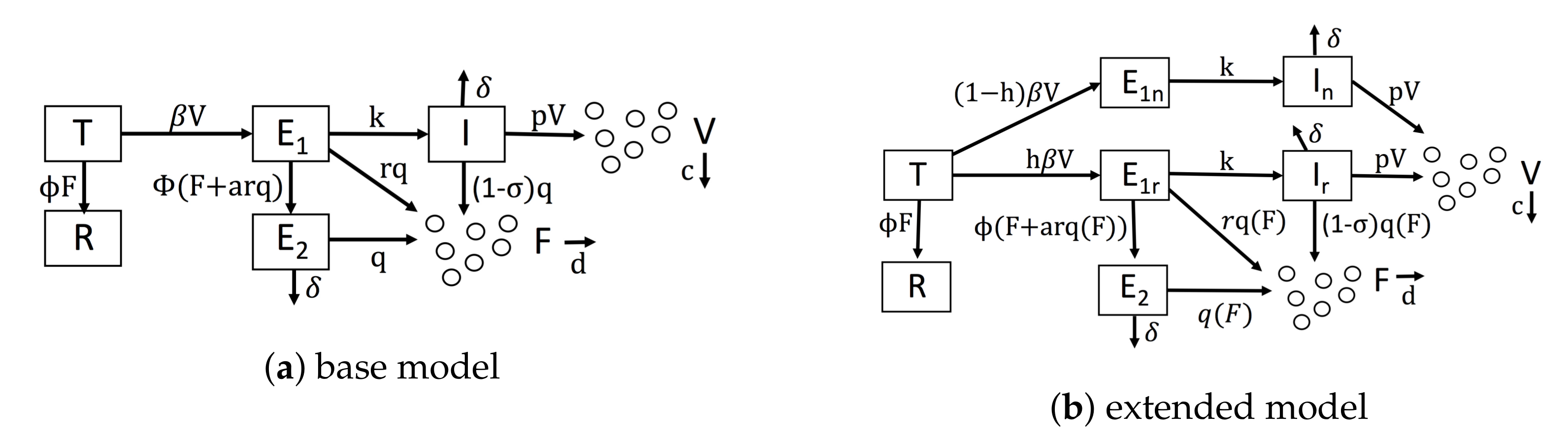
Figure 1.
Diagrams of our mathematical models. (a) Our base model, which is similar to Saenz et al.’s model. (b) Our extended model, which accounts for IFN feedback and heterogeneity. IFN feedback is modeled through the function , which gives the secretion rate as a function of extracellular IFN concentration. Heterogeneity is modeled through the parameter h, which gives the fraction of target cells capable of inducing IFN.
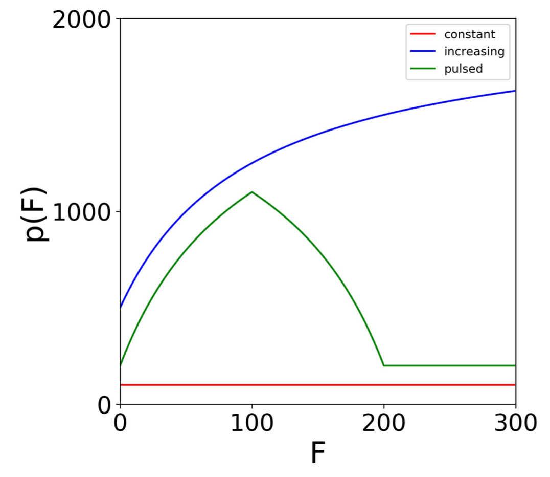
Figure 2.
Secretion rate models. Profiles for the constant (), increasing (, , ) and the pulsed (, , ) secretion rate models. The models specify the cellular secretion rate () as a function of the extracellular IFN level (F). For the increasing and pulsed model, . For the pulsed model, the maximum secretion rate is achieved at .
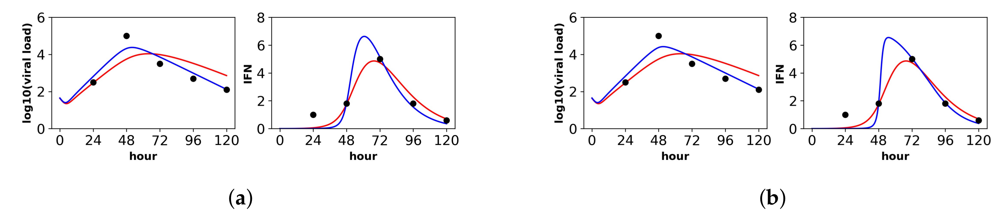
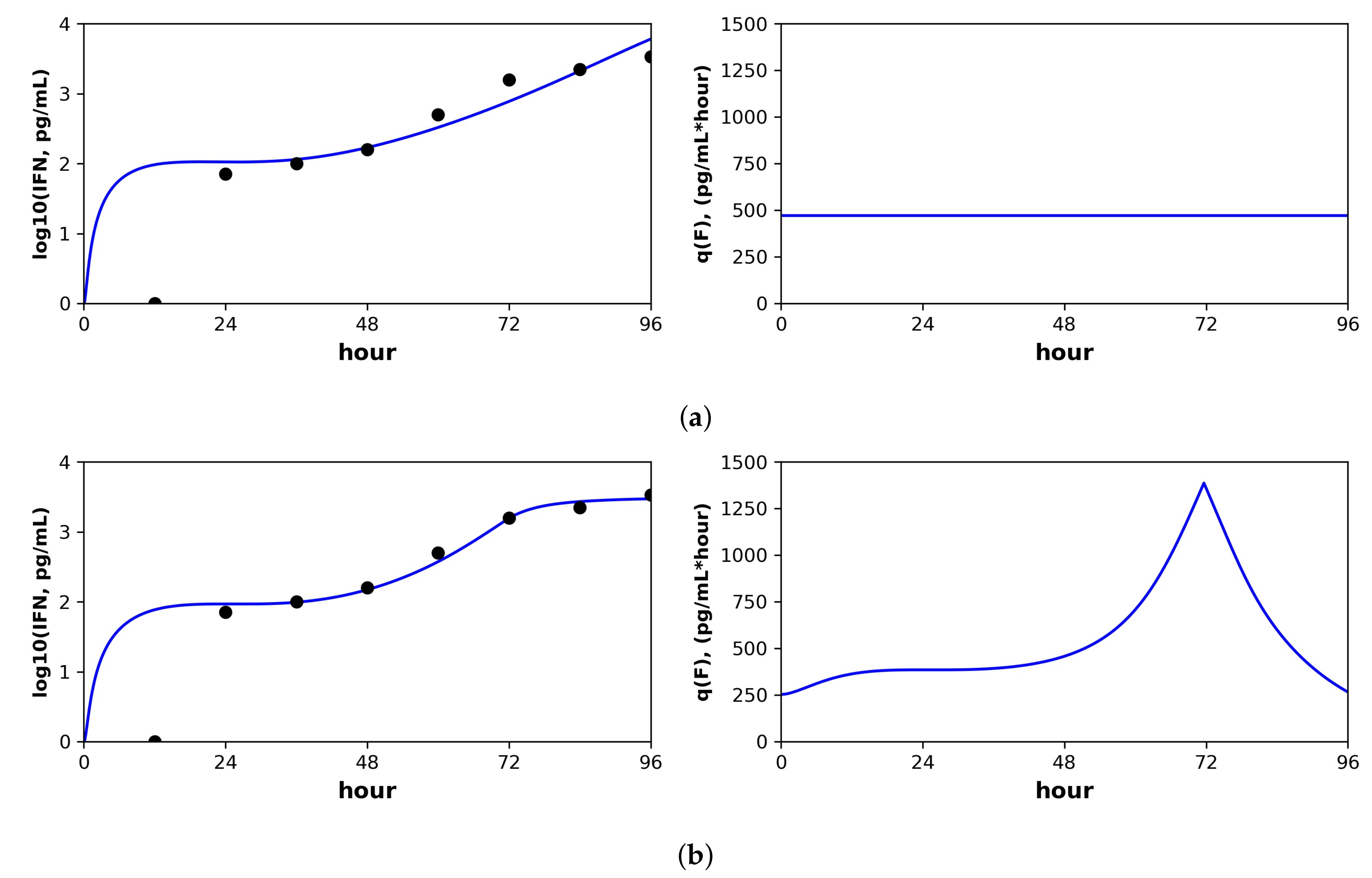
Figure 3.
Fit of the extended model to Saenz et al.’s dataset. Shown is the fit of our extended model (blue), assuming a (a) constant secretion rate and a (b) pulsed secretion rate, and the fit of the Saenz et al. model (red). Our secretion rate models give comparable fits, but the pulsed model suggests faster increases in IFN concentrations.
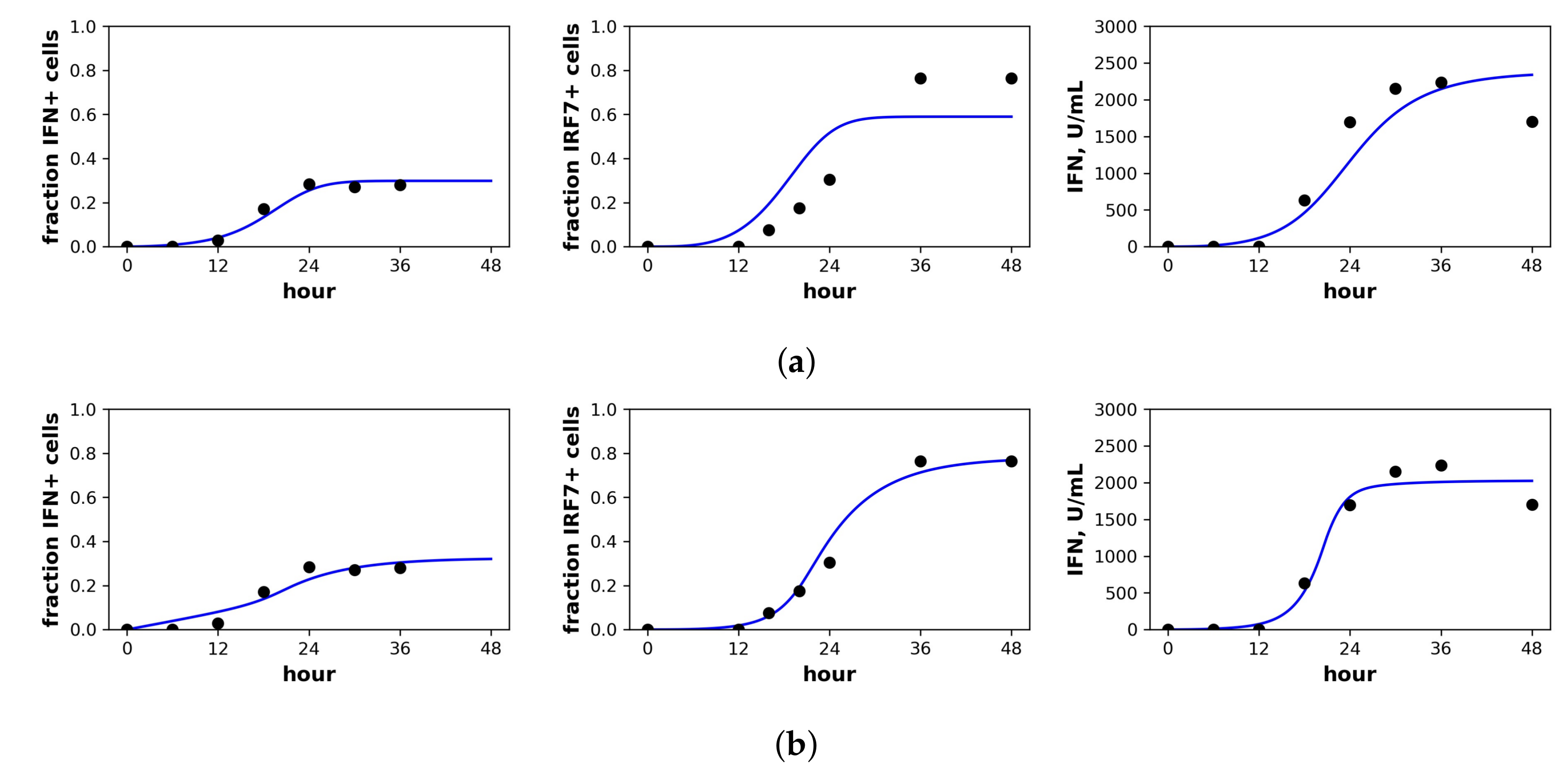
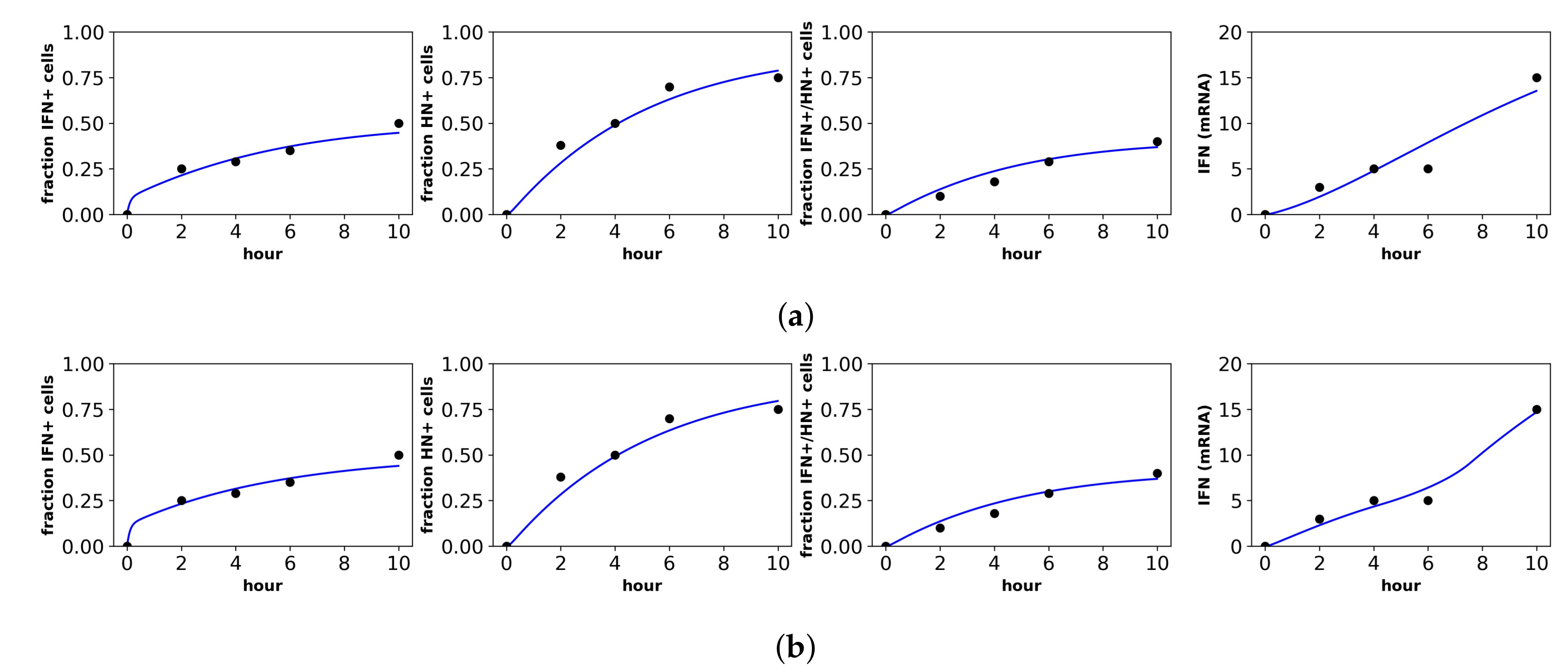
Figure 4.
Fit of the extended model to Rand et al.’s dataset. Shown is the fit of our extended model assuming a (a) constant secretion rate and (b) pulsed secretion rate model. Panels, from left to right, show the fraction of cells expressing IFN mRNA, IRF7 mRNA and the extracellular IFN concentration. The pulsed rate model captures the rapid increase in IFN concentrations between 12 h and 24 h.
Figure 5.
Fit of the extended model to Patil et al.’s dataset. Shown is the fit of our extended model assuming the (a) constant secretion rate and (b) pulsed secretion rate. Panels, from left to right, show the fraction of cells expressing IFN mRNA, viral HN, both IFN mRNA and viral HN and the average IFN mRNA expression across all cells.
Figure 6.
Constant versus pulsed rate secretion model predictions of interferon dynamics for the mutant (MT) dataset of Schmid et al. Shown are the predicted (blue curve) and sampled (black dots) IFN concentration dynamics (left panels) and the predicted IFN secretion rate dynamics (right panels) under our best fit model assuming (
a) constant secretion rate and (
b) pulsed secretion rate. Parameter values are shown in
Table 6. Fits to the complete Schimd et al. MT dataset are provided in the
Supporting Information, see
Figures S1 and S2.
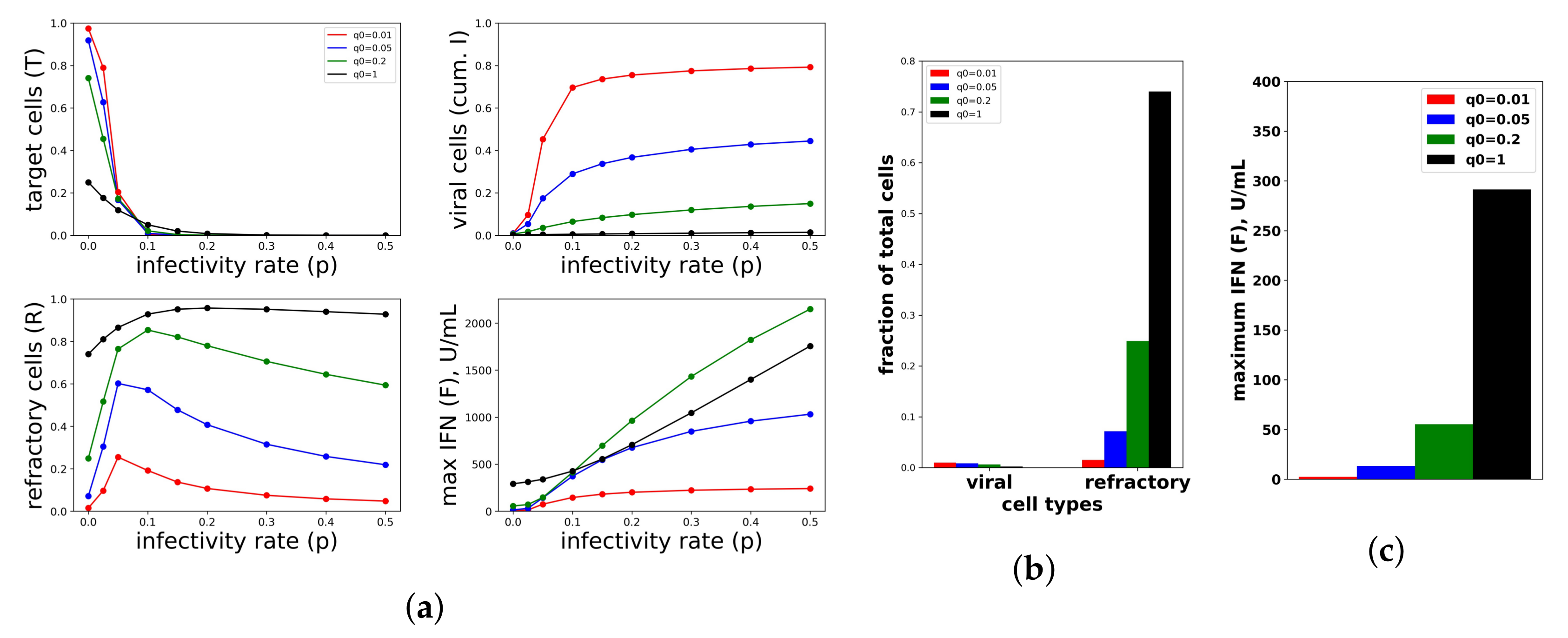
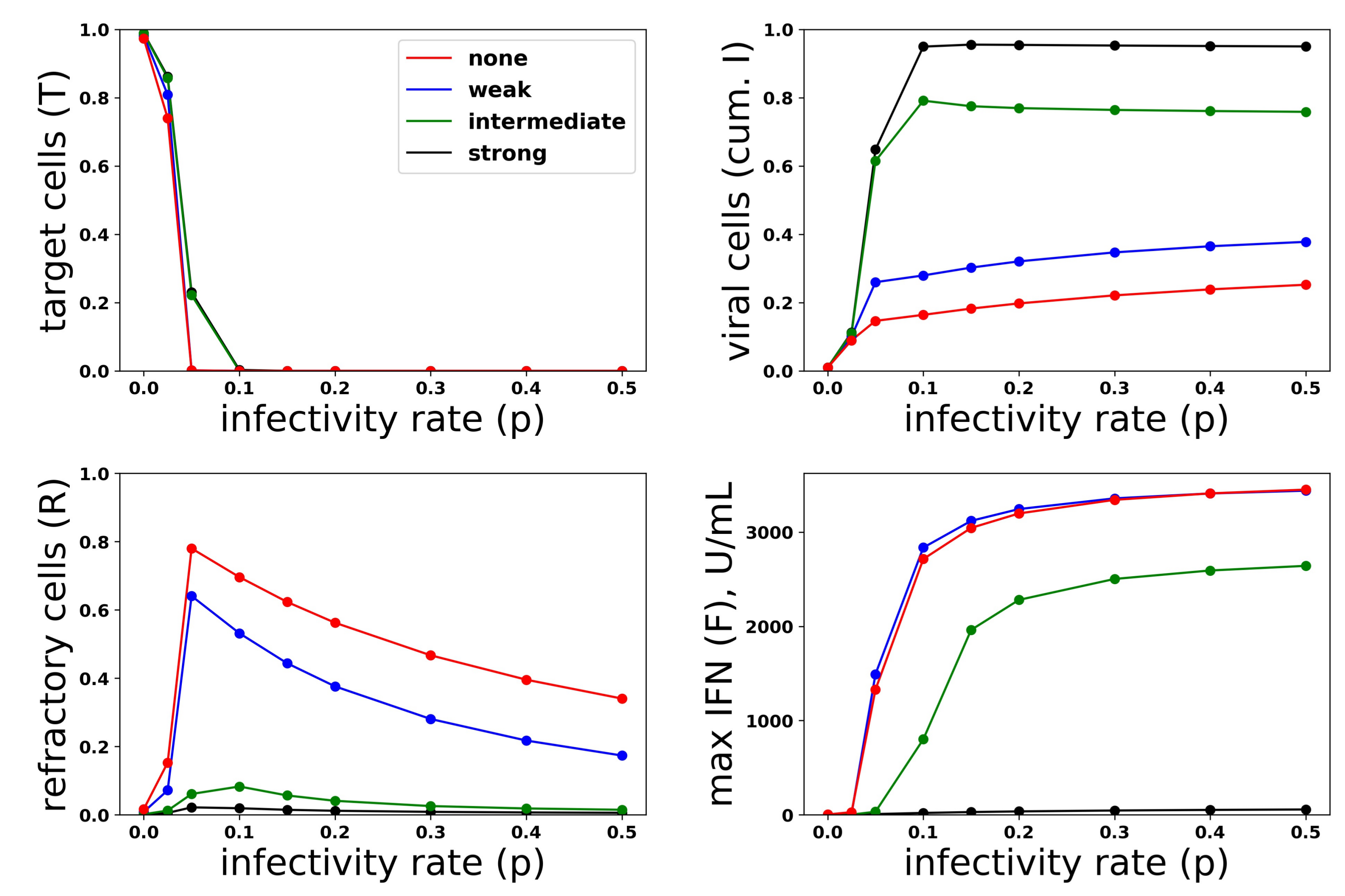
Figure 7.
A constant IFN secretion rate cannot simultaneously protect against high infectivity viruses and avoid excessive IFN secretion against low infectivity viruses. (a) Shown are the frequency of target cells, T, at the end of infection (top left), the fraction of cells that became virally productive, which is the cumulative number of cells in compartment I (top right), the total frequency of refractory cells, R, at the end of infection (bottom left), and the maximum of the extracellular IFN concentration, F, over the course of infection in U/mL (bottom right) as the viral infectivity rate p is varied. Each colored curve corresponds to a different , the IFN secretion rate, as specified in the legend. As p increases, protection requires relatively high values. Panels (b,c) are a zoom in of the results in Panel (a) for , representing an abortive infection. As the secretion rate varies, the number of virally-productive cells does not change significantly, but the fraction of refractory cells and the maximum IFN concentration levels rise considerably, reflecting excessive IFN secretion. Parameter values not shown: , , , , , , , , , .
![Viruses 10 00517 g007]()
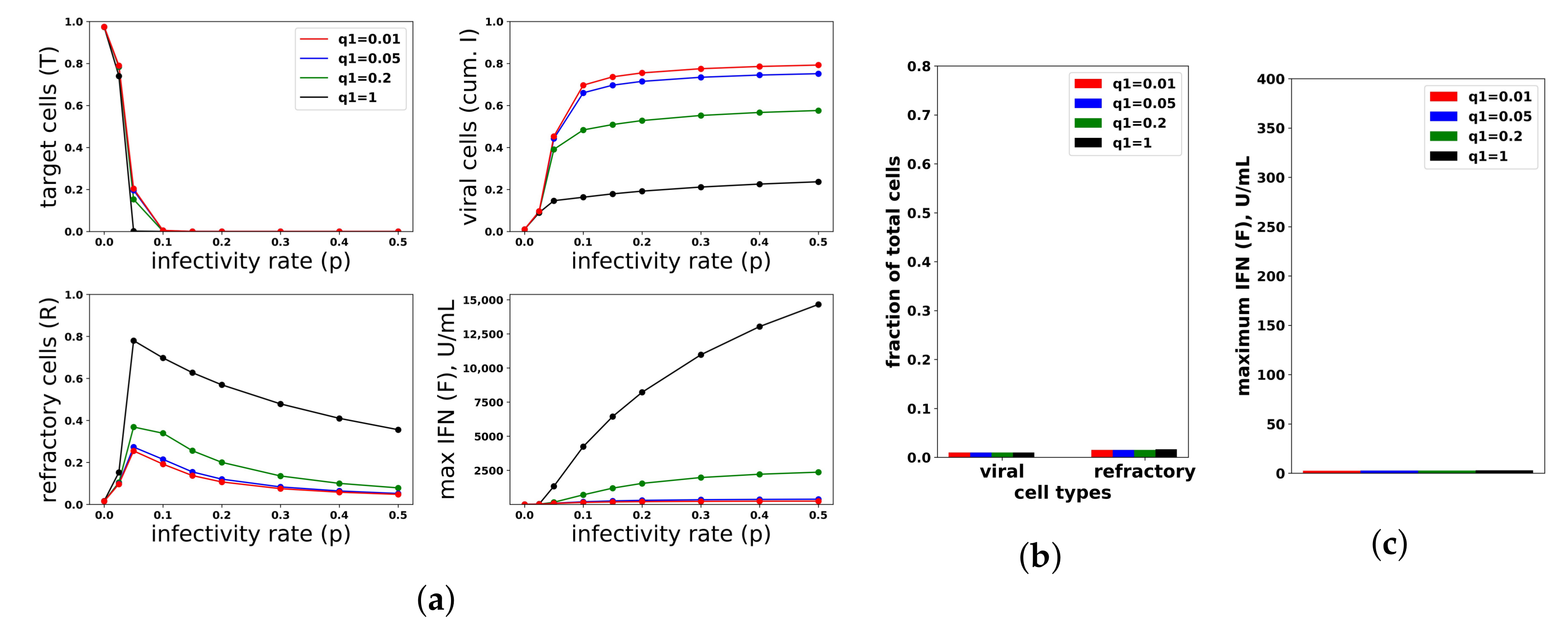
Figure 8.
An increasing IFN secretion rate can simultaneously protect against high infectivity viruses and avoid excessive IFN secretion against low infectivity viruses. This figure is analogous to
Figure 7, except that an increasing secretion rate is assumed. Each colored curve and bar correspond to a different value of
(see legend), and we fixed
. Compare Panels (
b,
c) of this figure and
Figure 7. See
Figure 7 for further details.
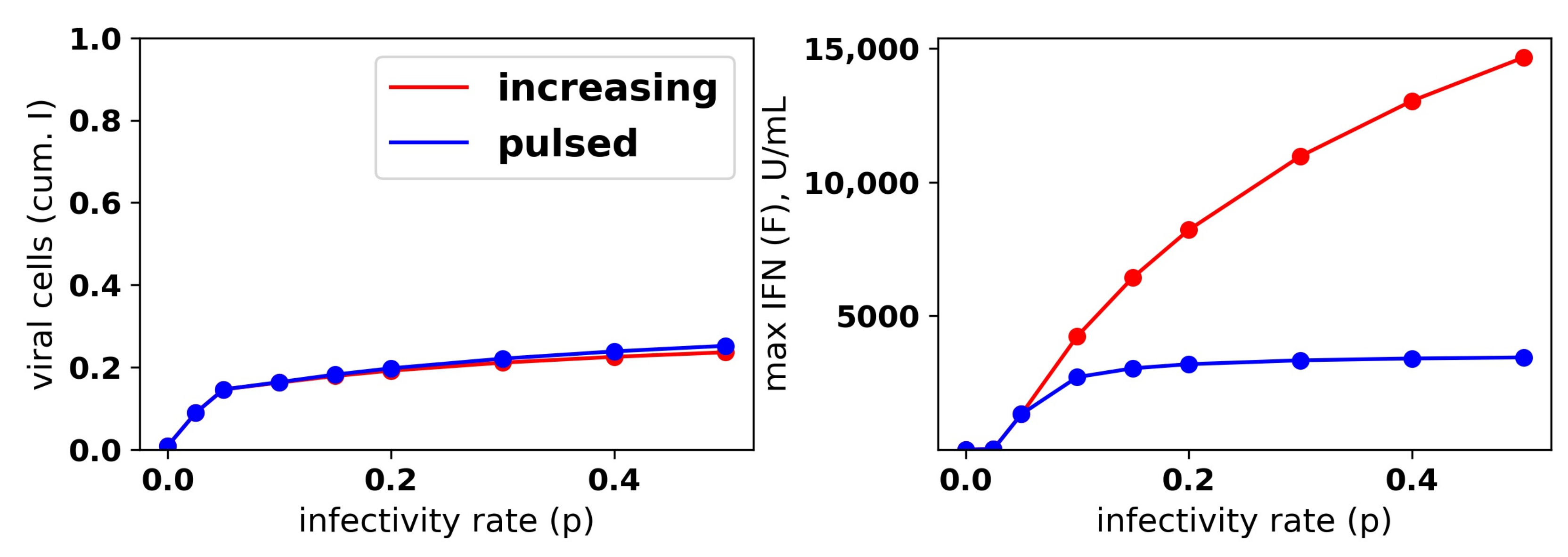
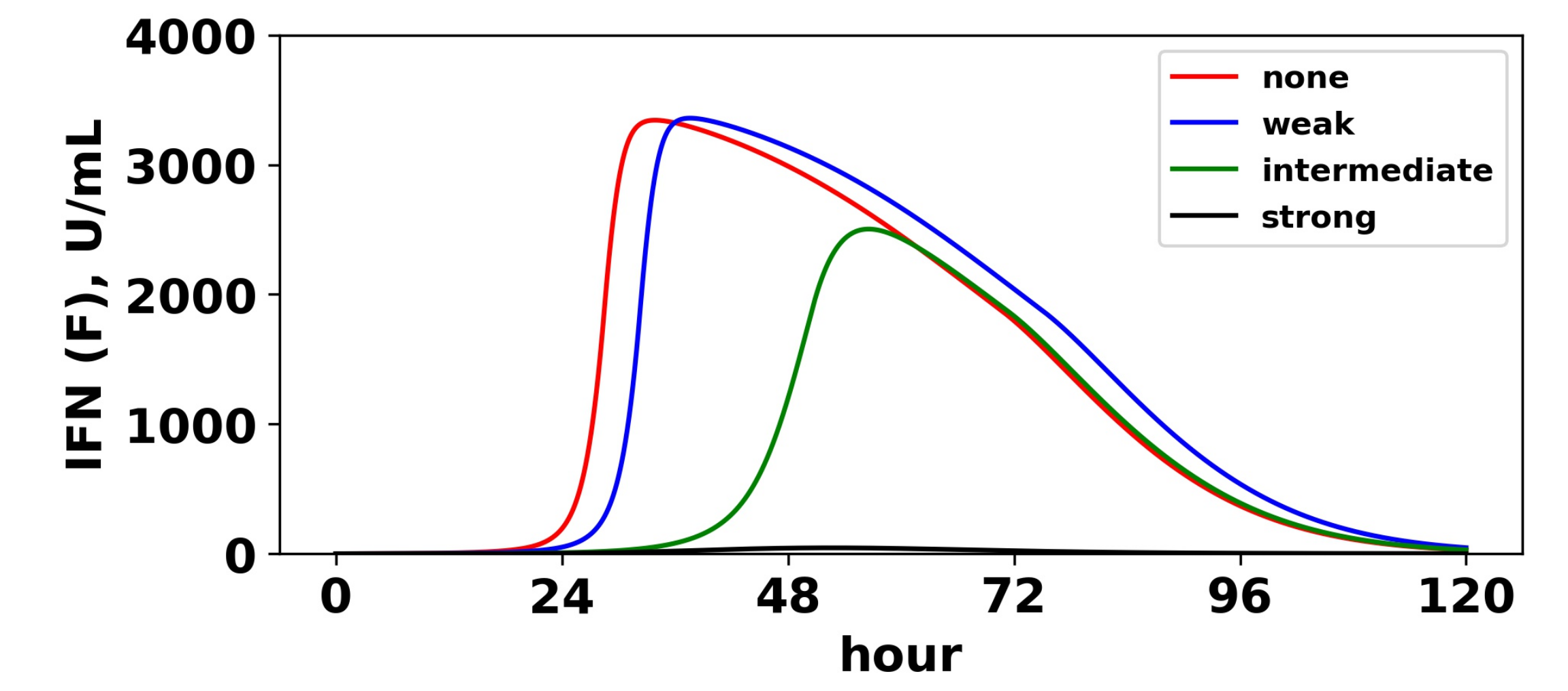
Figure 9.
A pulsed IFN secretion rate provides the same protection as an increasing IFN secretion rate, but with lower levels of extracellular IFN. See
Figure 8 and the text for details.
Figure 9.
A pulsed IFN secretion rate provides the same protection as an increasing IFN secretion rate, but with lower levels of extracellular IFN. See
Figure 8 and the text for details.
Figure 10.
Dynamics of the IFN positive feedback loop. Infection dynamics are shown for different infectivity rates p; see the legend. For each p, a pulsed secretion rate model was assumed. For , the feedback loop activates, leading to a rise in extracellular IFN concentrations (F) and a concordant transformation of target cells (T) into refractory cells (R) and the end of infection. For , the feedback loop does not activate. Dynamics were simulated using a pulsed secretion rate model with , , and .
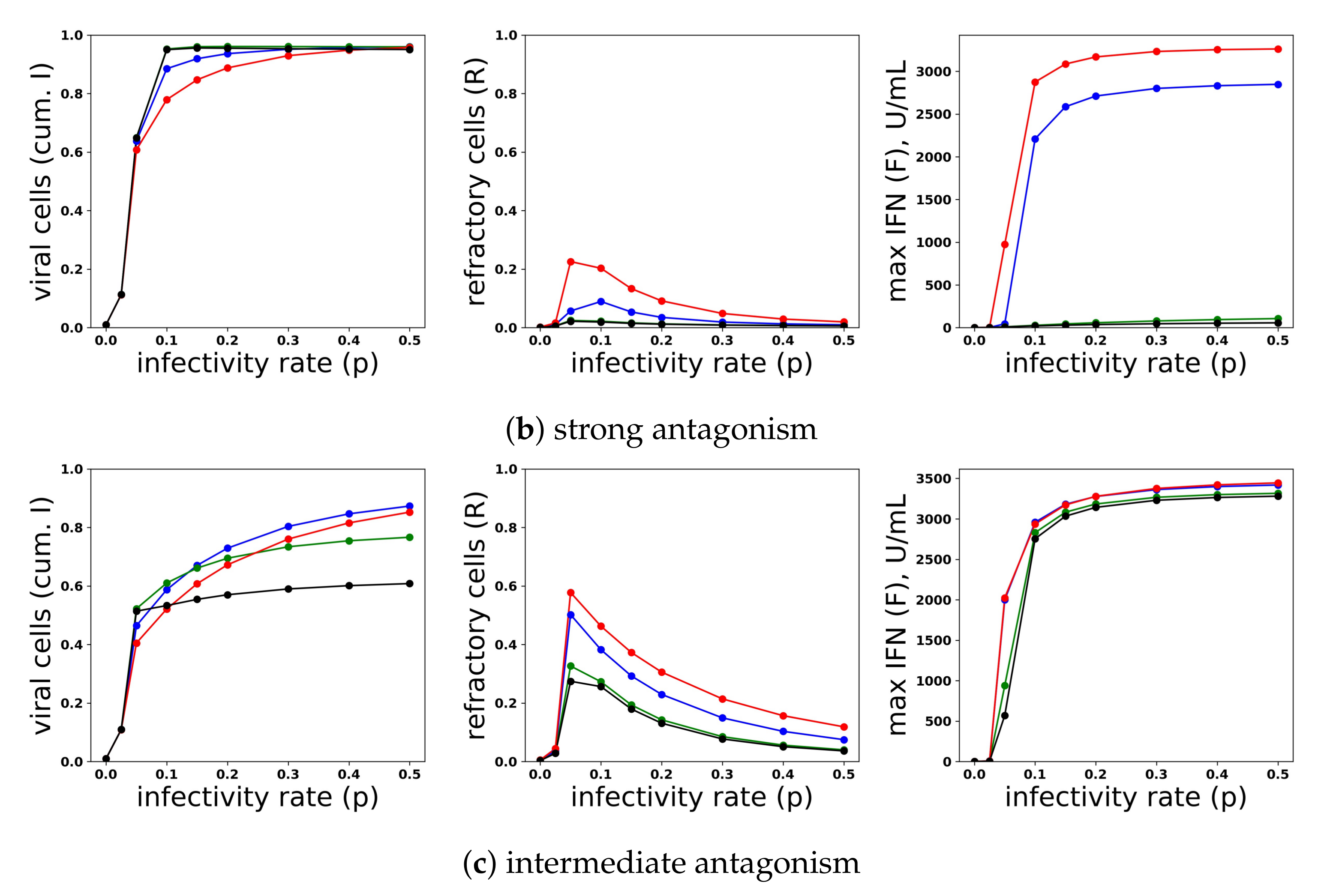
Figure 11.
Viral antagonism of IFN induction leads to loss of protection and can block the IFN feedback loop. Colored curves correspond to different levels of viral antagonism of IFN: , (none), , (weak), , (intermediate) and , (strong). When viral antagonism is strong, extracellular IFN concentration stay low, reflecting blockage of the feedback loop, while for intermediate antagonism maximal, IFN concentrations rise to the significant level, but do not mediate protection. For other levels of antagonism, extracellular IFN concentrations reach high levels, reflecting activation of the feedback loop, and the IFN response mediates significant protection.
Figure 12.
Viral antagonism of IFN induction delays activation of the feedback loop. Extracellular IFN levels (
F) are shown for four levels of IFN induction antagonism. For all levels, we set
, and we assumed a pulsed secretion rate model with
and
. As the level of antagonism is increased, activation of the feedback loop is delayed, and in the case of strong antagonism, the feedback loop is blocked. The delay or blockage of activation leads to the loss of protection, as shown in
Figure 11.
Figure 13.
A heterogeneous response provides protection against viral antagonism of IFN induction without excessive IFN secretion for low infectivity viruses. Using model simulations, we compared infection outcome across different levels of heterogeneity for a pulsed secretion rate model. (a) When no antagonism is present, infection outcome is similar for different levels of heterogeneity, although the homogeneous response () provides the best protection. (b) Under strong antagonism, the homogeneous IFN response and heterogeneous IFN response at () are blocked, while more heterogeneous responses () provide protection. (c) Under intermediate antagonism, all levels of heterogeneity provide protection, but higher levels of heterogeneity provided better protection.
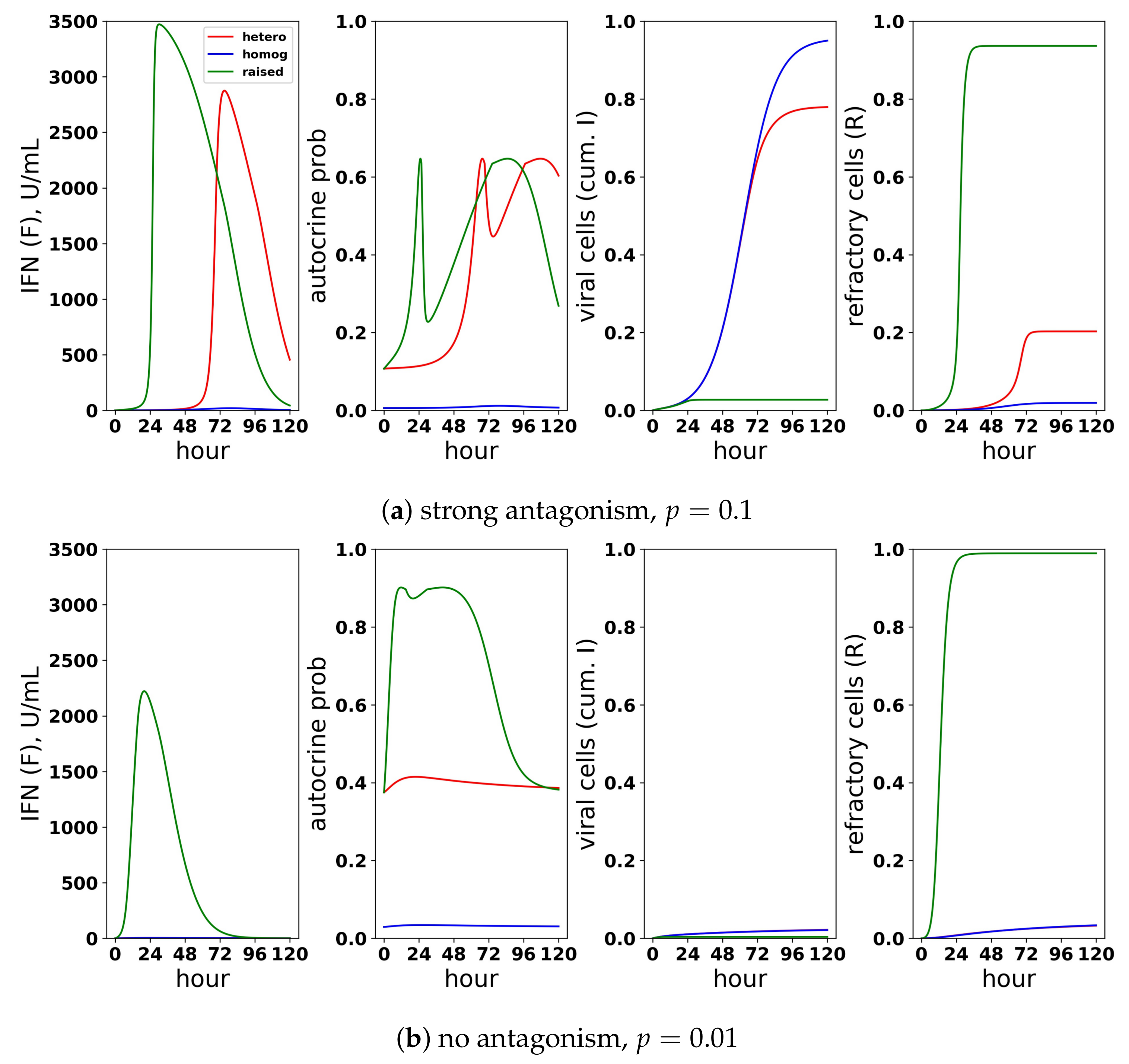
Figure 14.
A scaled heterogeneous response protects eclipse cells through autocrine-mediated signaling, while not excessively raising paracrine-mediated signaling to target cells. We considered a scaled heterogeneous response, a homogeneous response and a response in which we raised secretion rates, but did not restrict the fraction of cells that could induce IFN. (a) In the presence of strong antagonism and an infectivity rate , the feedback loop is activated, and extracellular IFN concentration rises for the heterogeneous and raised responses, but not for the homogeneous response. Rising extracellular IFN levels are mediated by strong autocrine signaling, which leads to a high probability that eclipse cells transform into effector cells (autocrine prob). Activation of the feedback loop leads to a lower frequency of viral cells and a higher frequency of refractory cells, particularly for the raised response. (b) In the absence of antagonism and an infectivity rate , the heterogeneous and homogeneous feedback loops do not activate, but the feedback loop activates for the raised response. For all three responses, viral cells have low frequency, but the raised response transforms nearly all target cells into refractory cells and raises extracellular IFN levels to 2000 U/mL, reflecting excessive IFN secretion.
![Viruses 10 00517 g014]()
Table 1.
Identifiability characteristics of the fitted parameters. We categorize each fitted parameter as structural non-identifiable (structural), practically non-identifiable (practical) or identifiable.
Table 1.
Identifiability characteristics of the fitted parameters. We categorize each fitted parameter as structural non-identifiable (structural), practically non-identifiable (practical) or identifiable.
| | Constant Rate Model | Pulsed Rate Model |
|---|
| Dataset | Structural | Practical | Identifiable | Structural | Practical | Identifiable |
|---|
| Rand et al. | | h | | | , , | |
| Saenz et al. # | | | | | | |
| Patil et al. | | | | | | |
| Schmid et al. (MT) | | | | | | |
| Schmid et al. (WT) | | | | | | |
Table 2.
Model parameters Units for IFN varied between datasets: Schmid et al. (IFN-lambda, pg/mL), Rand et al. (IFN-beta, U/mL), Saenz et al. (IFN-alpha, mRNA/mL), Patil et al. [
47] (IFN-beta, mRNA/mL).
Table 2.
Model parameters Units for IFN varied between datasets: Schmid et al. (IFN-lambda, pg/mL), Rand et al. (IFN-beta, U/mL), Saenz et al. (IFN-alpha, mRNA/mL), Patil et al. [
47] (IFN-beta, mRNA/mL).
| Parameter | Symbol | Units |
|---|
| baseline IFN secretion rate | | IFN/mL(hour) |
| upregulation IFN secretion rate | | IFN/mL(hour) |
| IFN upregulation constant | | IFN/mL |
| viral infectivity rate | | mL/virus(hour) |
| IFN protection rate | | mL/IFN(hour) |
| autocrine IFN fraction | a | |
| eclipse cell IFN secretion fraction | r | |
| viral and effector cell clearance rate | | 1/h |
| eclipse to viral cell transformation rate | k | 1/h |
| virion production rate | p | virus/hour |
| virion clearance rate | c | 1/ |
| extracellular IFN clearance rate | d | 1/h |
| fraction of target cells that can induce IFN | h | |
| viral antagonism level | | |
Table 3.
Fitted parameters for Rand et al.’s dataset under constant and pulsed secretion rate models. Parameters not shown were set to values determined in Rand et al; see
Table S1 in the Supporting Information. SSE is the sum of squared errors. Confidence intervals are at
level. IFN units are U/mL, and viral load units are HN/mL; see
Table 2 for the units of each parameter.
| Parameter | Constant | Pulsed |
|---|
| 1190 [1030,1390] | 100 [30,570] |
| | 5420 [3620,∞) |
| | 1120 [990,1320] |
| [, ] | [, ] |
| [, ] | [, ] |
| r | 0.00403 [0,0.88] | 0.37 [0.14,0.68] |
| h | 0.45 [0.38,1] | 0.66 [0.50,1] |
| (SSE) | 49.27 | 17.99 |
Table 4.
Fitted parameters for Patil et al.’s dataset under constant and pulsed secretion rate models. Confidence intervals are at the level. IFN and viral units are in terms of mRNA/mL.
Table 4.
Fitted parameters for Patil et al.’s dataset under constant and pulsed secretion rate models. Confidence intervals are at the level. IFN and viral units are in terms of mRNA/mL.
| Parameter | Constant | Pulsed |
|---|
| [6,9] | [2,13] |
| | 0 [0,7] |
| | [,∞] |
| ∞ [,∞] | ∞ [,∞] |
| [0,] | [0,] |
| k | [,∞] | [,∞] |
| r | [0,1] | [,1] |
| h | [,] | [,] |
| (SSE) | | |
Table 5.
Fitted parameters for the Saenz et al. dataset under constant and pulsed secretion rate models. Confidence intervals are at the level. IFN and viral units are in units of mRNA/mL.
Table 5.
Fitted parameters for the Saenz et al. dataset under constant and pulsed secretion rate models. Confidence intervals are at the level. IFN and viral units are in units of mRNA/mL.
| Parameter | Constant | Pulsed |
|---|
| [,] | [,∞] |
| | [0,∞] |
| | [0,∞] |
| r | [0,] | [0,1] |
| p | 44,800 [308,00,63,100] | 45,400 [0,69,000] |
| h | 1 [,1] | 1 [,1] |
| 1 [,1] | 1 [0,1] |
| (SSE) | | |
Table 6.
Fitted parameters for the Schmid et al. wild-type and mutant datasets under constant and pulsed secretion rate models. IFN and viral units are in terms of pg/mL and a.u./mL, respectively.
Table 6.
Fitted parameters for the Schmid et al. wild-type and mutant datasets under constant and pulsed secretion rate models. IFN and viral units are in terms of pg/mL and a.u./mL, respectively.
| Parameter | Wild-Type | Mutant |
|---|
| Constant | Pulsed | Constant | Pulsed |
|---|
| 95 [70,∞] | 58 [40,∞] | 470 [300,∞] | 250 [100,∞] |
| | 810 [200,∞] | | 2520 [970,∞] |
| | 95 [39,170] | | 1490 [100,2420] |
| [,] | [,] | [,] | [,] |
| [,] | [,] | [,] | [,] |
| r | 0 [0,] | [0,1] | 1 [,1] | 1 [,1] |
| p | 840 [450,1390] | 3000 [1280,11,020] | 580 [280,1040] | 340 [100,880] |
| h | 1 [,1] | 1 [] | 1 [] | [,1] |
| 0 [0,] | [0,1] | 1 [0,1] | 1 [0,1] |
| (SSE) | | | | |
Table 7.
Parameters for datasets in effective units. Effective units allow for comparison of the IFN response across datasets. We define IFN effective units (iEU) and viral effective units (vEU) as the extracellular IFN concentration and virion concentration, respectively, necessary to reduce target cell frequency by 1 natural log during 1 h. Units are vEU/hour (p), iEU/hour ( and ) and iEU ().
| | Schmid WT | Schmid MT | | |
| | Constant | Pulsed | Constant | Pulsed | | |
| p | 0.01 [0.01,0.02] | 0.02 [0.02,0.03] | 0.007 [0.005,0.01] | 0.006 [0.004,0.009] | | |
| 0.001 [0.0008,0.001] | 0.0006 [0.0004,0.0009] | 0.004 [0.003,0.006] | 0.003 [0.002,0.004] | | |
| | 0.009 [0.006,0.01] | | 0.025 [0.012,0.046] | | |
| | 0.001 [0.0009,0.001] | | 0.015 [0.008,0.022] | | |
| | Rand | Saenz | Patil |
| | Constant | Pulsed | Constant | Pulsed | Constant | Pulsed |
| p | | | 0.3 [0.2,0.4] | 0.3 [0.2,0.5] | | |
| 0.3 [0.03,0.4] | 0.006 [0.002,0.01] | 0.7 [0.5,2.9] | 0.008 [0.00006,0.7] | 0.04 [0.00004,0.19] | 0.04 [0.0004,0.23] |
| | 0.3 [0.2,0.8] | | 1.9 [1.4,32.3] | | 0 [0,0] |
| | 0.07 [0.03,0.19] | | 0.56 [0,3.1] | | 0.025 [.00002,0.11] |


