Effect of Thinning on the Spatial Structure of a Larix gmelinii Rupr. Secondary Forest in the Greater Khingan Mountains

Abstract

Thinning is an important way to adjust and optimize the spatial structure of forests. The study of its impacts support a better understanding of the succession process of secondary forests after interference. To study the changes in forest spatial structure under different thinning intensities and stand densities, we considered five thinning intensities including unthinned (0%), low (3.4%, 6.2%, 12.5%), medium (16.8%, 20.9%, 25.5%), high (34.4%, 40.0%, 47.9%), and extra-high (50.6%, 59.9%, 67.3%) intensity. In addition, three different stand densities for each degree of thinning intensity. The results showed that the most horizontal distribution patterns after thinning were uniform distribution and near-uniform random distribution. Most of the trees were not mixed while several were mixed to an above medium degree. The effect on dominance of thinning was not significant and the overall plots were in the middle level. The tree density was in the sparse status. Competitive pressure on the reference tree was reduced. Thinning intensity and stand density affected stand spatial structure to different degrees. There were no obvious pattern under different thinning intensities and it was optimal at approximately 1600 trees/ha. As thinning intensity increased, the impact tended to decrease first and then increase under certain stand density. The improvement was greatest when thinning intensity was low. By analyzing the stand’s spatial structure after thinning, the unreasonableness of the stand’s spatial structure can be found, which provides the basis for optimizing management measures. We used the AHP-entropy to weigh the importance of each spatial structure parameter and we proposed a comprehensive distance evaluation index based on the optimal value obtained in order to perform a comprehensive evaluation of a forest’s spatial structure.

1. Introduction

The forest in the Greater Khingan Mountains is a secondary community, which evolved from the degradation of the original top plant community after the interference of humans and nature primarily through overcutting and fire [1,2]. Compared to the old-growth forest, the original forest habitat has been lost in the secondary forest and there are significant differences in forest species composition, forest growth, forest productivity, the forest environment, and ecological function [3], which seriously restrict and affect the sustainable development of the forest. As the center of forest function, changes in forest structure affect the variation within a given stand. Only when the forest structure is optimized can the forest maintain a healthy and stable state. Then forest function can be given full play [4,5]. In the process of forest management, the spatial distribution and pattern within a forest are often adjusted to improve species composition and structural diversity [6,7,8]. Therefore, it is particularly important to study the optimization of a secondary forest’s structure and function.

At present, many descriptions of forest spatial structure exist. One such description relies on traditional forest management and classical vegetation ecology theory, describes the forest’s spatial structure at different scales through statistical techniques, and takes individual forests as statistical units. Statistical indicators such as Ripley’s K function, the O-ring function, Fisher’s species diversity index, Pielou’s segregation index, and the aggregation index are commonly used [9,10,11,12,13,14]. Other descriptions present a quantitative analysis of forest spatial structure based on the relationship between neighboring trees, which expresses the distribution pattern of reference trees and their nearest neighboring trees at a specific scale. The method could enable managers to better understand the structure of a forest’s microenvironment and make quantitative adjustments to the forest structure accordingly [15]. At present, the complete spatial structure parameter system is composed of four structural parameters including the uniform angle index [16], dominance [17], mingling [18], and crowding [19]. These parameters represent tree species diversity and the interspecific isolation degree, horizontal distribution pattern, forest competition status, and the forest crowding degree. Many studies of the spatial structure of forests have been carried out by using these indexes [20,21,22,23]. Secondary forest succession varies from that of a virgin forest. In general, the natural succession of a secondary forest is thought to conform to the naturally convergent rule in secondary succession [24]. However, artificial interference may lead to reverse development. At present, we know little about the influence of thinning on the spatial structure of Larix gmelinii Rupr. secondary forests and there is little research on the influence of related disturbance on the formative mechanism and evaluative process of a typical secondary forest.

After thinning, the most intuitive changes are those in forest density and the microenvironment of the forest. Many studies have focused on the changes in soil chemical and physical properties, litter water-holding capability, stand leaf area, and photosynthetic response [25,26,27,28,29,30]. These ecophysiological aspects greatly affect the growth of trees and indirectly affect the spatial structure of individual stands. Most of the current studies stem from two perspectives: (1) the analysis of the spatial structure following thinning of different forest densities when thinning intensity is certain and (2) the analysis of the spatial structure following different thinning intensities in forests with similar densities. To better study the changes in a forest’s spatial structure under different conditions, this paper proposes two hypotheses: (1) tree density and thinning intensity both affect the spatial structure of the Larix gmelinii secondary forest and (2) the spatial structure parameters will change as stand density and thinning intensity change. We propose a comprehensive distance evaluation index on a weighting of each spatial structure parameters (mingling, uniform angle index, dominance, and crowding), which can comprehensively evaluate the effect of all four parameters on the spatial structure after thinning.

2. Materials and Methods

2.1. Study Area

The study area is located in the Xinlin forest farm, Xinlin forestry bureau, and the research plots, which were established in compartment 106–109 (Figure 1). The site is flat with the slope under 6° and the elevation ranges from 540 to 603 m. The soil is brown forest soil and the average soil thickness is 14 cm. The site is located in a warm, temperate continental climate with an annual average temperature of 2.6 °C, a maximum temperature of 37.9 °C, and a minimum temperature of −46.9 °C. The annual precipitation is 513.9 mm and is concentrated in July and August. The annual average frost-free period is approximately 90 days. The annual sunshine hours are 235.7 h and the percentage of sunshine is 51% to 56%. Annual average wind speed is usually 2 to 3 m/s and occurs primarily in May. The main tree species is Larix gmelinii with a small number of Populus davidiana Dode, Betula platyphylla Suk., Pinus sylvestris var. Mongolica Litv. as well. Primary shrubs include Rhododendron dauricum L. and Lespedeza bicolor Turcz., which provide approximately 30% coverage. Underground herbaceous and liana species are dominated by Vaccinium vitis-idaea Linn., which represents 65% of herbaceous and liana abundance.

2.2. Plot and Field Survey

In March 2007, 13 forest plots were established in the research area and numbered 1~13. No. 1 was unthinned and served as the control (Figure 1). The forest environment factors such as gradient, slope aspect, and stand type were similar for all plots. The silvicultural interventions for all plots before thinning were focused on the cutting of shrubs and herbs, which seriously affected the growth of target species and sapling. Thinning intensity was based on the ratio of logged volume to total volume in accordance with timber forest management requirements, which govern cutting of trees in larger stand densities, no growth trees, and non-target species. Thinning intensities were as follows for each plot: 0%, 3.4%, 6.2%, 12.5%, 16.8%, 20.9%, 25.5%, 34.4%, 40.0%, 47.9%, 50.6%, 59.9%, and 67.3%. Forest densities varied under each thinning intensity grade (

Table 1. General characteristics of the plots.

Plot	Thinning Intensity (%)	Before Thinning Volume (m3·ha−1)	After Thinning Volume (m3·ha−1)	Tree Density (TreeNumber·ha−1)	Mean DBH (cm)	Average Height (m)	Average Crown Breadth (m)
1	0	105.6	105.6	2175	10.79	11.37	1.19
2	3.4	83.7	80.8	2325	10.49	11.32	1.47
3	6.2	83.4	78.2	2175	10.63	10.39	1.30
4	12.5	106.4	93.1	1675	11.70	12.23	1.44
5	16.8	111.5	92.9	1650	12.03	12.56	1.34
6	20.9	77.3	61.1	1125	13.07	12.62	1.63
7	25.5	102.7	76.6	1575	11.92	12.04	1.24
8	34.4	131.3	86.2	2050	11.20	11.30	1.15
9	40. 0	146.4	87.8	1950	11.40	11.38	1.26
10	47.9	84.5	44.0	1275	14.02	12.62	1.08
11	50.6	124.3	61.4	1525	12.33	12.36	1.35
12	59.9	155.9	62.5	1150	11.77	13.12	1.34
13	67.3	179.7	58.9	1200	12.67	12.96	1.08

DBH is the Diameter at Breast Height.

). In August 2017, we investigated all trees (DBH (diameter at breast height) of 1.3 m) ≥5 cm and recorded DBH, tree height, crown width, tree species, and location.

2.3. Data Analysis

2.3.1. Analysis 1—Stand Spatial Structure

We selected four parameters to analyze the stand spatial structure including the uniform angle index (W), dominance (U), mingling (M), and crowding (C) (

Table 2. Definitions and values for each spatial structure index.

Index	Formula	Value
		0	0.25	0.5	0.75	1
W	$W_i=\frac{1}{4}{\displaystyle \sum _{j=1}^4{z}_{ij}}$	Absolutely uniform	Uniform	Random	Nonuniform	Clumped
U	$U_i=\frac{1}{4}{\displaystyle \sum _{j=1}^4{k}_{ij}}$	Predominant	Subdominant	Moderate	Inferior	Extremely inferior
M	$M_i=\frac{1}{4}{\displaystyle \sum _{j=1}^4{v}_{ij}}$	Not mixed	Weakly mixed	Medium mixed	Strongly mixed	Extremely strongly mixed
C	$C_i=\frac{1}{4}{\displaystyle \sum _{j=1}^4{y}_{ij}}$	Extremely sparse	sparse	Moderately dense	Relatively dense	Extremely dense

). The uniform angle index describes the horizontal distribution of neighboring trees [16,31,32]. Dominance describes the degree of size difference between neighboring trees and reference trees [17,33]. Mingling describes the degree of spatial isolation of tree species relative to other species [18,34,35] and crowding describes the density of trees and the forest canopy layer’s coverage [19,36]. The formulas used are shown below.

The z_ij expresses whether the angle (α) of an adjacent tree compared to the reference tree is less than the standard angle α₀ (α₀ = 72°), if α < α₀, z_ij = 1. Otherwise, z_ij = 0. The average W reflects the overall level of the forest relative to three distributions: random, clumped, and uniform, which occur between (0.475, 0.517), above 0.517 and below 0.475, respectively. When the nearest neighbor is larger than the reference tree, k_ij = 1. Otherwise, k_ij = 0. When the species of the nearest neighbor is not the same as the reference tree, v_ij = 1. Otherwise, v_ij = 0. y_ij expresses whether the canopy projection of the reference tree overlaps that of the adjacent tree. If yes, y_ij = 1. Otherwise, y_ij = 0.

2.3.2. Analysis 2—Determining Weight of Spatial Structure Parameters

The spatial structure parameters are not only independent but also related to each other. They affect one another. Therefore, the four parameters must be analyzed together to understand a forest’s spatial structure and more fully represent the spatial functional quality of a forest. At present, some scholars rely on the evaluation index of the stand spatial structure, which uses the multiplication division method, the stand spatial structure index, and an evaluation index of the distance applying input-output function to comprehensively evaluate a stand’s spatial structure [37,38,39]. However, these indexes are all based on the premise that the structural parameters contribute equally to an ideal spatial structure, which does not illustrate the role of each parameter in the spatial structure. Therefore, it is necessary to determine the contribution of each forest spatial structure parameter to an ideal spatial structure and weigh each parameter accordingly [40]. There are many methods for weighing techniques including the analytic hierarchy process (AHP), the grey correlation method, the entropy weight method, principal component analysis, and the multi-objective programming approach. The most widely used method is the AHP, which is systematic, simple, and practical. However, because the subjective consciousness is strong, we combined the AHP with the entropy weight method to determine the weight. The entropy method is adaptable to any process that requires weight determination and can be used in combination with some methods. We can easily get the objective weight when compared to the principal component analysis and grey correlation [41,42,43]. The combination of the subjective and objective weights resulted in a more reasonable evaluation result.

The analytic hierarchy process (AHP) was used to determine the subjective weight of each spatial structure parameter. The problem was deconstructed into different components and a hierarchical analysis structure model (target layer-criterion layer) was established according to the degree of membership. First, a pairwise comparative judgement matrix (Equation (1)) was constructed by taking advantage of the importance of each structural parameter to the target layer (c_ij). Second, the formula Aw = λw was used to obtain the eigenvector corresponding to the maximum eigenvalue (λ_max) and the eigenvector was normalized to be the weight vector. The consistency test was conducted for the single hierarchical order, according to Equation (2) and Equation (3). If it passed the test, the weight vector obtained was used as the weight of each index. Otherwise, the judgement matrix was adjusted. The m represents the number of evaluation indexes, m = 4, RI (average random consistency index) value was 0.90.

$$A=\left[\begin{array}{cccc}{c}_{11}& c_{12}& \cdots & c_{1m}\\ c_{21}& c_{22}& \cdots & c_{2m}\\ ⋮& ⋮& \ddots & ⋮\\ c_{m1}& c_{n2}& \cdots & c_{mm}\end{array}\right]$$

(1)

$$CI=\frac{{\lambda }_{\max }-m}{m-1}$$

(2)

$$CR=\frac{CI}{RI}$$

(3)

The entropy method was used to determine the objective weight of each spatial structure parameter, which is based on the index variability. The smaller the entropy value, the more information the index provides and the greater the role it plays in decision-making. This method makes the weight obtained more objective and reasonable. After standardizing the measured data (Equation (4)), the judgement evaluation matrix (R_ij) was created. Equation (5) was used to obtain the information entropy and the weight of each indicator was obtained by using the information entropy (Equation (6)).

$$R_{ij}=\frac{x_{ij}-\min (x_{ij})}{\max (x_{ij})-\min (x_{ij})}+1$$

(4)

where x_ij is the raw data and n is the number of evaluation ratings. i = 1,2,···, m; j = 1,2,···, n.

$$E=-\frac{1}{\ln (n)}{\displaystyle {\sum }_{j=1}^n{p}_{ij}}\ln (p_{ij})$$

(5)

where $p_{ij}=\frac{r_{ij}}{{\displaystyle {\sum }_{j=1}^n{r}_{ij}}}$

$$u_i=\frac{1-E}{{\displaystyle {\sum }_{i=1}^m(1-E)}}$$

(6)

The comprehensive weight is obtained by combining the subjective weight (w) and the objective weight (u) (Equation (7)).

$$C{W}_i=\frac{w_i{u}_i}{{\displaystyle {\sum }_{i=1}^m{w}_i{u}_i}}$$

(7)

The mean value of each spatial structure index may reflect the overall forest, but it cannot embody the spatial distribution of the forest interior. Therefore, we used the preference value proposed by Chai [44] to describe the distance between the real state of the forest and its ideal state. Of the four indexes, the uniform angle index, and crowding are intermediate indexes where the optimal value (O) is 0.5. The dominance parameter is a negative index with an optimal value (O) of 0 and the mixing parameter is a positive index with an optimal value (O) of 1.

$$PV=1-\sqrt{\frac{{\displaystyle {\sum }_{j=1}^n{(I_j-O)}^2}}{n}}$$

(8)

where PV is the preference value and I_j is the index value of spatial structure.

The result of the comprehensive distance evaluation (CDEV) is the sum of the product of the weight and preference values, as described in Equation (9). The greater the comprehensive value is, the better the forest spatial structure is.

$$CDEV={\displaystyle {\sum }_{i=1}^m(C{W}_i}\times P{V}_i)$$

(9)

The raw data were processed in Excel 2007 and SPSS 20.0 was used for the analysis of the one-way ANOVA, checking whether there are significant differences among all plots. We used R software (version 3.4.4) to analyze the forest spatial structure and the comprehensive distance evaluation including the spatstat package and forestSAS package [44].

3. Results

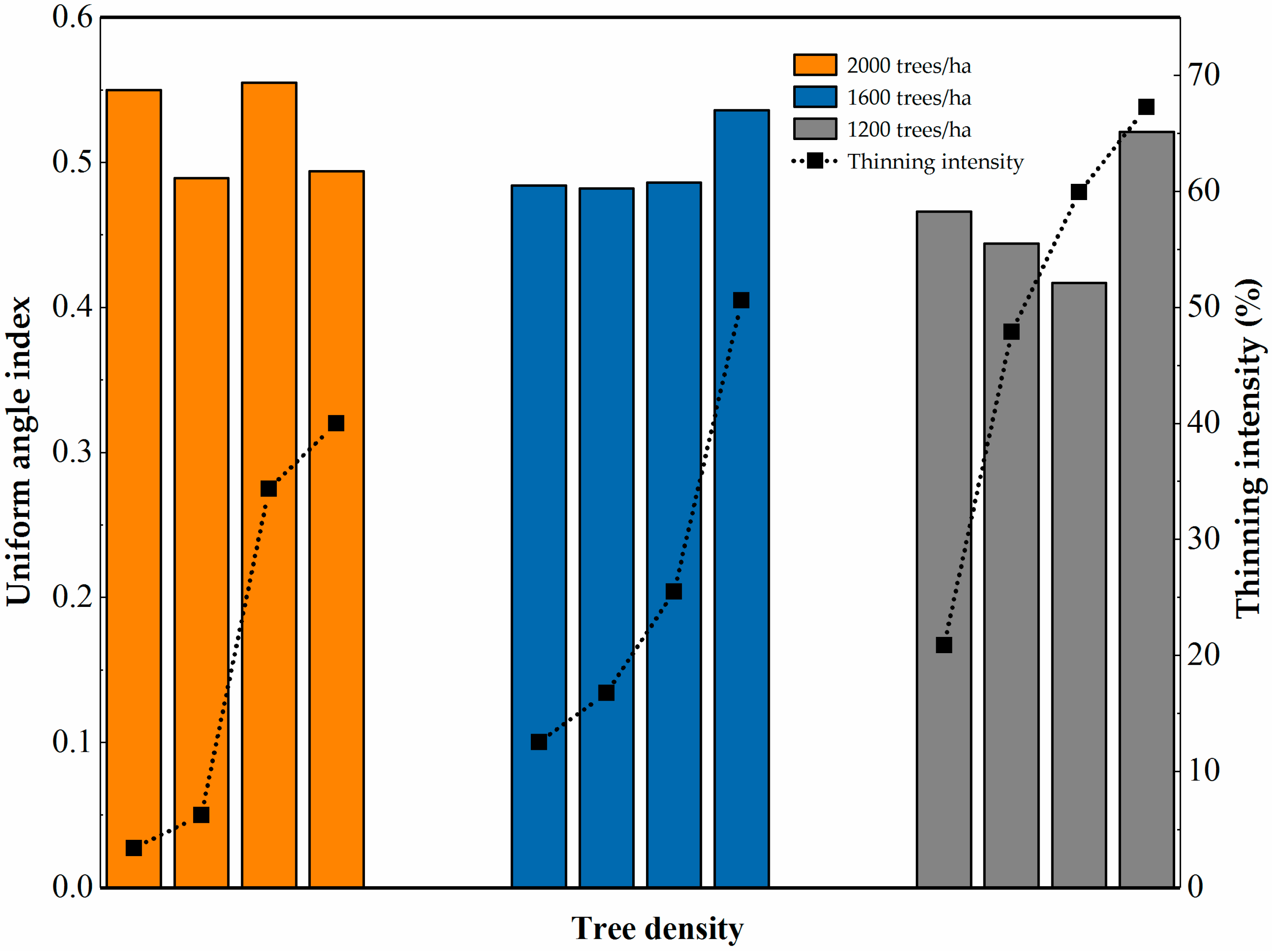
3.1. Effects of Thinning on the Uniform Angle Index

For the uniform angle index (

Table 3. Frequency distribution and mean value of W in different plots.

Plot	Value					$\overline{\mathit{W}}\pm \mathit{S}$
	0	0.25	0.5	0.75	1
1	0.008	0.165	0.614	0.118	0.094	0.531 ± 0.207ab
2	0.000	0.160	0.540	0.240	0.060	0.550 ± 0.196 b
3	0.000	0.273	0.523	0.182	0.023	0.489 ± 0.186ab
4	0.000	0.273	0.523	0.182	0.023	0.484 ± 0.157ab
5	0.000	0.25	0.607	0.107	0.036	0.482 ± 0.179ab
6	0.000	0.182	0.773	0.045	0.000	0.466 ± 0.117ab
7	0.000	0.227	0.568	0.205	0.000	0.486 ± 0.215ab
8	0.024	0.195	0.439	0.220	0.122	0.555 ± 0.247b
9	0.071	0.071	0.500	0.357	0.000	0.494 ± 0.166ab
10	0.000	0.333	0.556	0.111	0.000	0.444 ± 0.167ab
11	0.000	0.226	0.613	0.161	0.000	0.536 ± 0.216ab
12	0.000	0.381	0.571	0.048	0.000	0.417 ± 0.144a
13	0.000	0.171	0.629	0.143	0.057	0.521 ± 0.187ab

$\overline{W}$ was the average value of the W, S is the standard deviation. Different lowercase letters indicate significant differences among different plots (p < 0.05).

), there were no significant differences found except in plots 2, 8, and 12. The average W in plots 3, 4, 5, 7, and 9 were in the range of (0.475, 0.517). The distributions were random, but the values were low and near a uniform distribution. The average values found for plots 6, 10, and 12 were 0.466, 0.444, and 0.417, which were under 0.475. This indicates that the horizontal distributions within these plots were uniform. The distributions within the other plots were clumped. For the frequency distribution of five values, the number of the absolutely uniform distribution (W = 0) and the clumped distribution (W = 1) were small indicating that most of the plots were near zero. The frequency of the uniform distribution (W = 0.25) was greater than 0.2 in most of the plots. Trees with a random distribution (W = 0.5) exceeded 0.5 and the frequency of a non-uniform distribution (W = 0.75) was greater than 0.1. There were no clear changes occurring with an increase in thinning intensity. The average W were lower than that in the unthinned plot for all plots except 2, 8, and 11. At medium thinning intensities (plots 5, 6, 7), W first increased and then decreased as the tree density decreased. In the other thinning intensity plots, W decreased gradually with a decrease in tree density. When the stand density is constant, the value decreased first and then increased with the increase of thinning intensity. The average value decreased as stand density decreased (Figure 2).

3.2. Effects of Thinning on Dominance

No significant differences were found for the dominance in any of the plots after thinning (

Table 4. Frequency distribution and mean value of U in different plots.

Plot	Value					$\overline{\mathit{U}}\pm \mathit{S}$
	0	0.25	0.5	0.75	1
1	0.189	0.157	0.220	0.220	0.213	0.528 ± 0.352a
2	0.220	0.160	0.280	0.140	0.200	0.485 ± 0.355a
3	0.205	0.227	0.159	0.250	0.159	0.483 ± 0.351a
4	0.194	0.278	0.222	0.194	0.111	0.468 ± 0.346a
5	0.321	0.143	0.107	0.286	0.143	0.446 ± 0.381a
6	0.136	0.227	0.136	0.364	0.136	0.534 ± 0.330a
7	0.159	0.250	0.182	0.273	0.136	0.438 ± 0.324a
8	0.146	0.220	0.268	0.171	0.195	0.512 ± 0.335a
9	0.214	0.214	0.214	0.214	0.143	0.494 ± 0.330a
10	0.111	0.222	0.222	0.222	0.222	0.556 ± 0.349a
11	0.194	0.226	0.290	0.097	0.194	0.464 ± 0.352a
12	0.190	0.238	0.143	0.286	0.143	0.488 ± 0.349a
13	0.229	0.229	0.171	0.171	0.200	0.471 ± 0.368a

$\overline{U}$ was the average value of the U, S is the standard deviation. Different lowercase letters indicate significant differences among different plots (p < 0.05).

). Dominance values ranged from (0.438, 0.556) and the proportion of overall dominant trees was moderate. At the same time, there was no significant difference in the frequency distribution under the five values. Except for plots 6 and 10, the average U of all plots was lower than that of the unthinned plot. Average dominance decreased with the decrease in tree density in low thinning intensity plots. In the case of the medium and high thinning intensity plots, average U first increased and then decreased as the tree density increased with minimum values occurring in plots 5 (1650 trees/ha) and 11 (1500 trees/ha), which indicates that the number of reserved trees had an impact on dominance. At high thinning intensities, the trend first decreased and then increased with the minimum value occurring in plot 9 (1950 trees/ha). When the tree density was about 2000 trees/ha and 1200 trees/ha, the value first increased and then decreased with increasing thinning intensity and the trend was opposite to the change of value when the density was approximately 1600 trees/ha (Figure 3).

3.3. Effects of Thinning on Mingling

After thinning, the degree of mingling in each plot was found to be between zero and moderate with values ranging from (0.00, 0.372) (

Table 5. Frequency distribution and mean value of M in different plots.

Plot	Value					$\overline{\mathit{M}}\pm \mathit{S}$
	0	0.25	0.5	0.75	1
1	0.323	0.220	0.213	0.181	0.063	0.360 ± 0.488cd
2	0.400	0.380	0.040	0.040	0.140	0.285 ± 0.343cd
3	0.614	0.250	0.045	0.000	0.091	0.176 ± 0.298bc
4	0.167	0.472	0.139	0.167	0.056	0.371 ± 0.322d
5	1.000	0.000	0.000	0.000	0.000	0.000 ± 0.000a
6	0.545	0.182	0.136	0.091	0.045	0.227 ± 0.304cd
7	0.318	0.341	0.159	0.068	0.114	0.368 ± 0.283d
8	0.341	0.293	0.073	0.122	0.171	0.372 ± 0.376d
9	0.571	0.214	0.071	0.143	0.000	0.330 ± 0.325cd
10	0.889	0.111	0.000	0.000	0.000	0.028 ± 0.083ab
11	0.290	0.258	0.194	0.194	0.065	0.196 ± 0.280d
12	0.429	0.286	0.238	0.048	0.000	0.226 ± 0.236cd
13	0.457	0.286	0.114	0.114	0.029	0.243 ± 0.288cd

$\overline{M}$ was the average value of the M, S is the standard deviation. Different lowercase letters indicate significant differences among different plots (p < 0.05).

). Based on the frequency range of the five values, most plots exhibited zero to weak mixing with zero mixing generally predominate. Few trees were strongly or extremely strongly mixed. Significant differences were found between plot 5, plot 10, and the other plots. Both plots 5 and 10 exhibited near zero mixing. When the thinning intensity was low, the degree of mingling found in plots 3 and 4 differed from one another. When thinning intensity was high, no significant differences in mingling were found between any plots. For low thinning intensity, M first decreased and then increased as the tree density decreased. Average M decreased as the tree density increased in medium and extra-high thinning intensity plots, which is different when compared with the change in mingling in high thinning intensity plots. The mingling degree was higher when the tree density was approximately 2000 trees/ha and the M first decreased and then increased with the increase in thinning intensity (Figure 4).

3.4. Effects of Thinning on Crowding

Crowding differed significantly across plots (

Table 6. Frequency distribution and mean value of C in different plots.

Plot	Value					$\overline{\mathit{C}}$ ± S
	0	0.25	0.5	0.75	1
1	0.402	0.354	0.157	0.071	0.016	0.236 ± 0.249cd
2	0.160	0.320	0.340	0.160	0.020	0.390 ± 0.253ef
3	0.318	0.477	0.159	0.045	0.000	0.233 ± 0.205cd
4	0.444	0.333	0.194	0.028	0.000	0.476 ± 0.284f
5	0.607	0.250	0.143	0.000	0.000	0.134 ± 0.186abcd
6	0.545	0.182	0.273	0.000	0.000	0.182 ± 0.221bcd
7	0.341	0.318	0.273	0.045	0.023	0.201 ± 0.214bcd
8	0.317	0.488	0.098	0.073	0.024	0.250 ± 0.244d
9	0.500	0.286	0.214	0.000	0.000	0.273 ± 0.252de
10	1.000	0.000	0.000	0.000	0.000	0.000 ± 0.000a
11	0.161	0.129	0.419	0.226	0.065	0.179 ± 0.206bcd
12	0.619	0.381	0.000	0.000	0.000	0.095 ± 0.124abc
13	0.714	0.286	0.000	0.000	0.000	0.071 ± 0.115ab

$\overline{C}$ was the average value of the C, S is the standard deviation. Different lowercase letters indicate significant differences among different plots (p < 0.05).

). The average C in plot 10 was zero and exhibited extremely sparse characteristics while the remaining plots exhibited extremely sparse to moderately dense conditions ranging between (0.071, 0.476). This indicates that the competitive pressure of reference trees within the study forest was low. Most values were distributed between the extremely sparse and sparse categories (C = 0, 0.25) while the distribution of trees in the other crowding categories was minimal. Significant differences were found between plots 2, 3, 10, 13, and the unthinned plot. When the thinning intensity was low, average C varied between plot 3 and the others and when tree density decreased, average C first decreased and then increased. Plot 4 exhibited moderate crowding with a value close to 0.5. No significant differences in C were identified in the medium and extra-high thinning intensity plots. However, as the tree density decreased, the average C gradually increased in plots where medium thinning intensity was applied in direct contrast to plots where extremely high thinning intensity was applied. In the high thinning intensity plots, they varied between plot 10 and the others. It had the same trend when the tree density was about 1600 trees/ha and 1200 trees/ha (Figure 5).

3.5. Comprehensive Evaluation of Spatial Structure

First, we applied AHP in order to obtain subjective weights for each index relative to the forest’s spatial structure. We established a judgement matrix of the importance of the criterion layer relative to the target layer and then we obtained the eigenvalue and eigenvector using MATLAB (

Table 7. Result and consistency test of the data layers using AHP.

Evaluation Factors	Uniform Angle Index	Dominance	Mingling	Crowding
Uniform Angle Index	1	1/2	2	1
Dominance	2	1	3	1
Mingling	1/2	1/3	1	1/2
Crowding	1	1	2	1
Subjective Weight	0.233	0.365	0.125	0.277
Consistency Test	CI = 0.015 CR = 0.017

CI is the consistency index, CR is the consistency ratio of the judgement matrix.

). The maximum eigenvalue was 4.046, the consistency index CI was 0.015, and the consistency ratio of the judgement matrix CR was 0.017 <0.1. This indicated that the judgement matrix was consistent and did not need to be adjusted. The subjective weight for each index is shown in Table 7. Second, we used the entropy weight method to obtain objective weights for each index. Because zero values existed in the original data, the dataset needed to be treated with non-negative processing (Equation (4)). We obtained the objective weights for each indicator, which equalled 0.236, 0.267, 0.278, and 0.219 for W, U, M and C, respectively. Lastly, we combined the objective and subjective weights to derive a comprehensive weight for each parameter (Equation (7)): 0.22, 0.39, 0.14, and 0.24, respectively.

Table 8. Optimal distance evaluation of forest spatial structure in different thinning plots.

Plot	W.PV	U.PV	M.PV	C.PV	CDEV
1	0.792	0.366	0.285	0.638	0.516
2	0.800	0.401	0.209	0.726	0.542
3	0.815	0.405	0.125	0.665	0.521
4	0.843	0.408	0.299	0.755	0.574
5	0.823	0.418	0.000	0.591	0.491
6	0.881	0.376	0.171	0.616	0.518
7	0.788	0.458	0.309	0.634	0.554
8	0.750	0.390	0.271	0.653	0.518
9	0.836	0.408	0.256	0.663	0.544
10	0.833	0.355	0.025	0.500	0.450
11	0.789	0.425	0.152	0.622	0.516
12	0.836	0.405	0.193	0.577	0.513
13	0.815	0.436	0.151	0.517	0.500

W.PV, U.PV, M.PV, C.PV are the preference values of W, U, M, C, respectively. CDEV is the value of comprehensive distance evaluation.

showed the preference value of all indexes. The distribution of the overall uniform angle index was near the optimal value and all PV values were greater than 0.7. Followed by crowding, the PV was greater than 0.5 and the distance between the dominance, mingling, and optimal values was large. Under different thinning intensities, the variation in the PV was different from that of the index value. The PV of W and U had a significant negative correlation with the index value (>0.8), which indicates that the variation in the PV of these two indexes presented a contrary trend with the index value relative to the decrease in tree density. Only the high thinning intensity case was different. In that case, the PV of W first increased and then decreased with the decrease in tree density. The PV of M and C exhibited a significant positive correlation with the index value (>0.92) except that the PV of M tended to first increase and then decrease in the extra-high thinning intensity plot. Under different stand densities, the change in the PV of U opposed that of the index value (>0.75) while the PV of M matched that of the index value (>0.95). The PV of W had a significant negative correlation with the index value when the stand density was about 2000 trees/ha (>0.8). The PV of C had significant correlation with the index value when the stand density was approximately 1600 trees/ha and 1200 trees/ha (>0.93) while the other cases had no correlation with the index value.

The average PV of W under medium thinning intensity conditions was greater than that under other intensities, followed by low thinning intensity, extra-high thinning intensity, and high thinning intensity conditions. The average PV of U was greatest in the extra-high thinning intensity plots while it was the lowest in the high thinning intensity plots. The maximum PV of M and C appeared in the low thinning intensity plots and the average PV of C decreased as thinning intensity increased. The average PV of W increased with the decrease in tree density while the average PV of M and C decreased gradually with the decrease in tree density.

The CDEV for all plots was approximately 0.5 with the maximum occurring in plot 4 and the minimum occurring in plot 10 (Table 8). The average CDEV was greatest in the low thinning intensity plots followed by the medium, extra-high, and high thinning intensity plots, respectively. Under stand density, the average CDEV was greatest in the 1600 trees/ha and the trend was the same when the stand density was about 1600 trees/ha and 1200 trees/ha.

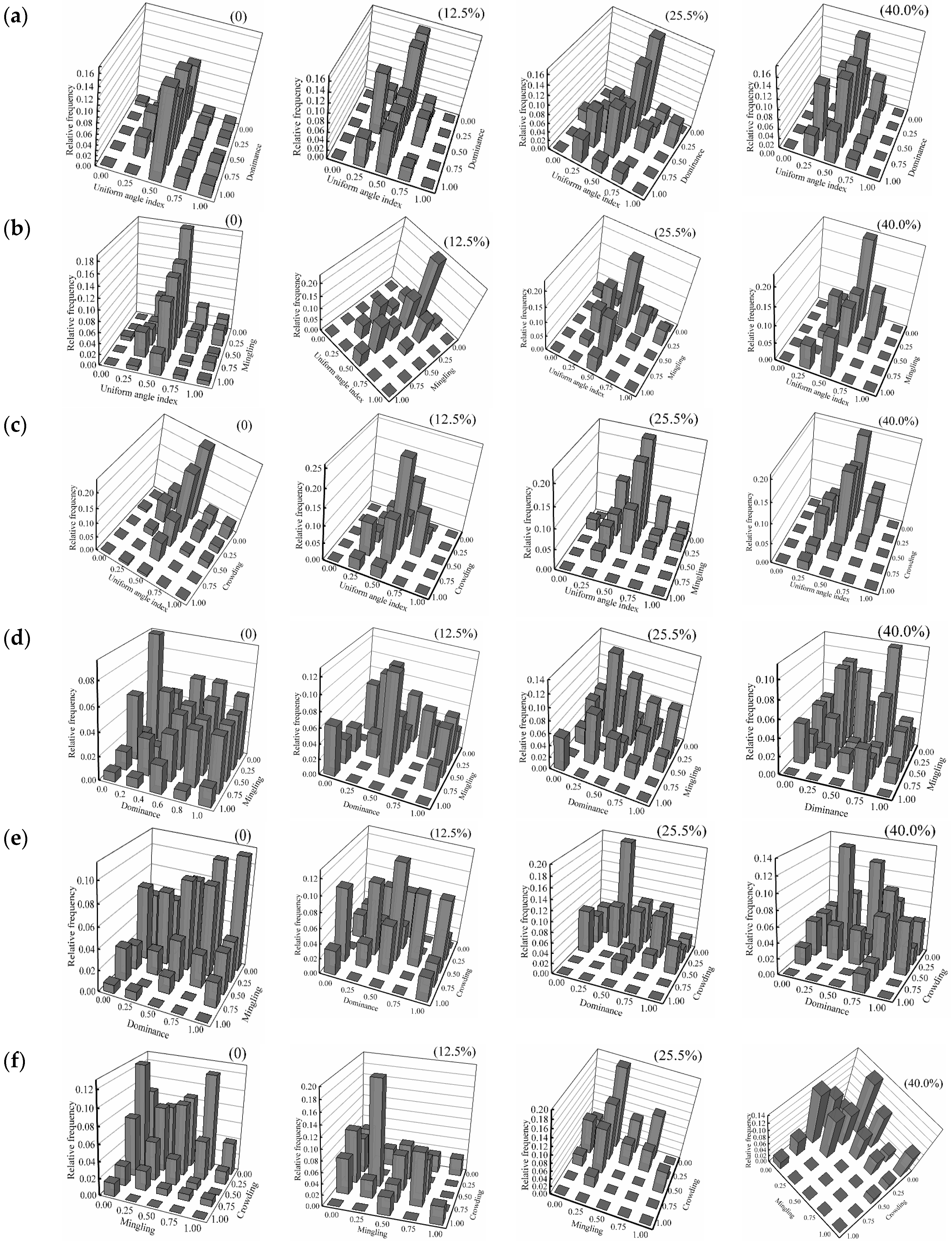
3.6. Bivariate Distribution of Spatial Structure

To better understand the relationship among the forest spatial structure indexes, this paper analyzed the binary distribution of the indexes for those plots with the greatest comprehensive evaluation values: 12.5%, 25.5%, and 40.0%. The unthinned plot was evaluated as well (Figure 6).

In the W-U bivariate distribution, we found that more than half (0.614, 0.613, 0.528, 0.568) of the plot distributions were random (W = 0.5). On the random distribution axis, there was a stark contrast between the test plots and the unthinned plot. Dominant (U = 0) and subdominant (U = 0.25) characteristics occurred most frequently while this frequency reached a maximum of U = 1 (0.165) in the unthinned plot. In terms of dominance, the minimum frequencies of thinned plots were obtained when U = 0.75 and U = 1. In the unthinned plot, the minimum value was reached when U = 0.25, and as distribution values increased, the frequency of U first increased and then decreased. When W = 1, all U values were distributed in the unthinned plot while, in the other plot, only some values were distributed.

In the W-M bivariate distribution, mingling within all plots was generally distributed at M = 0 and M = 0.25 when W = 0.5, which relates to the forest type. When the uniform angle index distribution value increased, the frequency first increased and then decreased even though it remained around W = 0.5. In the unthinned and low thinning intensity plots, the frequency of M decreased gradually as the distribution value increased.

In the W-C bivariate distribution, when W = 0.5, the distribution frequency of the low thinning intensity plot reached a maximum at C = 0.5 while that of the other plots was C = 0. As the distribution value increased, the frequency of C in the thinned plots tended to decrease. At the same time, compared to the unthinned plot, the distribution frequency (W = 0.25 and W = 0.75) increased in addition to W = 0.5.

In the U-M bivariate distribution, all combinations of U and M occurred in the unthinned plot. When U = 0, the frequency of M first decreased and then increased with the increase of the distribution value in the low and the medium thinning intensity plots, which reached a maximum value when M = 1. However, in the case of the unthinned and high thinning intensity plots, the frequency was almost 0 when M = 1. When M = 1, values were only distributed on U = 0 and U = 0.75 in the thinned plots while al U values were distributed in the unthinned plot and reached the maximum value when U = 0.5.

In the U-C bivariate distribution, the distributions within the four plots varied with the maximum frequency distribution occurring at U = 0.5 and C = 0.5, U = 0.25 and C = 0, U = 0.25 and C = 0.25, U = 1 and C = 0, respectively. On C = 0.75 and C = 1, the distribution of U seldom occurred in the medium and high thinning intensity plots. At the same time, when U = 0, the frequency first increased and then decreased as C increased in the medium thinning intensity plots. When C = 0.5, the patterns of each plot varied.

In the U-C bivariate distribution, the maximum value of the combination occurred when M = 0, 0.25 and C = 0.25, 0.25. When M = 1, it was distributed only at C = 0.5 in the medium thinning plot. Its frequency was 0 at C = 0.75 and C = 1 in the high thinning plot and the distribution of C = 0.5 in the other plots was 0. When C = 5 in the unthinned plot, the frequency of U decreased successively as the distribution value increased.

4. Discussion

The forest spatial structure determines the development of the forest function. A reasonable structure is necessary for a sustainable ecosystem management. Therefore, in order to manage a forest system, one must adjust that forest’s structure. Thinning is a primary natural forest management technique and plays an extremely important role in forest management. Research has shown that thinning leads to an increase in the forest space, reduces competition among individuals, and encourages tree growth [45,46,47]. Our results agree with these findings. Average DBH and tree height were greater in the vast majority of our study plots than in the unthinned plot. The forest spatial structure was re-adjusted after thinning and the environment changed. As a result, numerous feedback effects were generated. Therefore, a study of the change in spatial structure plays an extremely important role in understanding the impacts of thinning on forests and provides a reference for us to adjust forest management operations in the future.

Our results showed that the unthinned plot exhibited an aggregated distribution, moderate dominance, weak to medium mixing, and sparse crowding. Most of the plots after thinning exhibited uniform distribution to random distributions, which has been found in other studies [48,49,50]. Furthermore, the dominant position and crowding of trees were better in the thinned plots compared to the unthinned plot even though few trees exceed medium mixing. As tree density decreased, the variations in each index exhibited complex patterns under different thinning intensities. In the low thinning intensity plots (3.4% to 12.5%), the uniform angle index and dominance showed a decreasing trend and grew continually closer to an ideal state. Mingling and crowding showed a tendency to first decrease and then increase. All four indexes reached their optimal values when the tree density was approximately 1600 trees/ha. In the medium thinning intensity plots (16.8%–25.5%), the uniform angle index and dominance first decreased and then increased while the mingling and crowding index values increased. The uniform angle index reached an optimal state when the tree density was about 2000 trees/ha while the other indexes were optimized at 1600 trees/ha. In the extra-high thinning intensity plots (50.6%–67.3%), the index trends matched those of the medium thinning intensity plots except for crowding. In the high thinning intensity plots (34.4% to 47.9%), the uniform angle index and crowding gradually decreased. This result conflicts with the findings of Ye et al. [51] and is related to the forest type and forest management measures studied. Dominance first decreased and then increased and mingling first increased and then decreased. All indexes were near their ideal states at 2000 trees/ha. Based on the comprehensive evaluation index, we found that under the low, medium, and extra-high thinning intensity, the stand spatial structure can be improved when the tree density is approximately 1600 trees/ha. It was superior when tree density is approximately 2000 trees/ha in the high thinning intensity.

When tree density varied, the optimal situation for each indicator varied as well. When the tree density was approximately 2000 trees/ha, W, U, and M showed similar patterns. The average preference values of W, U, and C in the low thinning intensity plots were greater than the high thinning intensity plots while the value of M was better in the low thinning intensity plots. This may be because, at that density, the disturbance caused by low intensity thinning was minimal, thinning reduced tree species, and the mixing degree decreased. On the other hand, under high thinning intensity conditions, growth takes time to adjust and the feedback to the disturbance is not all positive and the thinning cannot improved the degree of crowding, the frequency of extremely sparse, and sparse were not increased, which is inconsistent with Li et al. [52]. When the tree density was approximately 1600 trees/ha, the preference value of W and M were all in the 12.5% thinning intensity. The other indexes were in the 25.5% thinning intensity and the comprehensive evaluation showed that the low thinning intensity was suitable in the 1600 trees/ha. When the tree density was about 1200 trees/ha, the preference value of U and M were in the extra-high thinning intensity. The final comprehensive evaluation still illustrated that the medium thinning intensity was better. In the process of studying the effect of stand density on the stand spatial structure, we acknowledged that the set of study plots was not complete. The primary reason for the lack of some research results was that the actual situation within the local plots varied and there were great difficulties setting up the samples used. The initial plots status as the initial volume or density shows a very large difference. For example, the volume ranges from 77 m³ to 179 m³. Therefore, the results of this study are still somewhat limited and cannot be fully determined by the effect of thinning intensity. In the future, we will try our best to control the influence of variables.

In structure-based forest management, the comprehensive evaluation of stand spatial structure parameters is imperative. Although detailed evaluations of stand spatial structure parameters exist, it is difficult for forest managers to quickly judge the effect of forest management. Thus, it is particularly important that we build a comprehensive evaluation model for forest managers to use. Different from the individual evaluation of indicators, the analysis results can more directly show whether a stand’s spatial structure is reasonable. The key step in the comprehensive evaluation developed in this study is to determine the weight of each indicator. We combined subjective and objective weights, which is a technique that has been applied in many studies and has a good evaluation effect [53]. The weights identified in this study are as follows: dominance (0.39) > crowding (0.24) > uniform angle index (0.22) > mingling (0.14). Zeng et al. found that the index weight is obtained by the relative importance of each index [54] and derived results that were very different from those found in this study. Therefore, largely, the identification of weight must reflect the specific local situation and the results for one area may not be applicable to any stand. However, this research opens up a new way to comprehensively evaluate the forest spatial structure in the future.

5. Conclusions

We examined the influence of thinning on the spatial structure of Larix gmelinii based on stand density and thinning intensity. We considered five treatments—low, medium, high, and extra-high intensities with unthinned as a control and three different stand densities in each treatment. Our findings provide that there were no significant differences in the uniform angle index or dominance among all plots while the differences in the mingling and crowding. Moreover, the dominance of the target species after thinning was homogeneous, the overall degree of mixing was low and species composition was limited to a single species. Overall, there was sufficient space for tree growth and more space and resources could be obtained for the individual. The horizontal distribution pattern of trees was uniform to near uniform random. Compared to the unthinned plot, the spatial structure of most of the plots improved after thinning.

A new comprehensive evaluation index of a stand’s spatial structure was established based on an optimal value. The proposed index can better express the distance to ideal spatial structure of the Larix gmelinii secondary forest in the Greater Khingan Mountains and objectively reflects the actual situation of the forest’s spatial structure. On the whole, the comprehensive evaluation indicated that it was beneficial with the low intensity and 1600 trees/ha. The Larix gmelinii secondary forest exhibits a generally medium level spatial structure and the spatial heterogeneity of the secondary forest is relatively low. Hence, the forest is still in a state of ecological recovery.

References

1. Ye, Y.; Fang, X. Land use change in Northeast China in the twentieth century: A note on sources, methods and patterns. J. Hist. Geogr. 2009, 35, 311–329. [Google Scholar] [CrossRef]
2. Yu, L.Z.; Liu, L.F.; Wang, X.G.; Sun, Y.R.; Kong, X.W.; Gao, T.; Li, X.F. Discussion on the protection and restoration technology of secondary forest ecosystems in Northeast China. Chin. J. Ecol. 2017, 36, 3243–3248. (In Chinese) [Google Scholar]
3. Zhu, J.J. A review on fundamental studies of secondary forest management. Chin. J. Appl. Ecol. 2002, 13, 1689–1694. (In Chinese) [Google Scholar]
4. Pretzsch, H. Analysis and modeling of spatial stand structures methodological considerations based on mixed beech-larch stands in Lower Saxony. For. Ecol. Manag. 1997, 97, 237–253. [Google Scholar] [CrossRef]
5. Pastorella, F.; Paletto, A. Stand structure indices as tools to support forest management: An application in Trentino forests. J. For. Sci. 2013, 59, 159–168. [Google Scholar] [CrossRef]
6. Comas, C.; Palahí, M.; Pukkala, T.; Mateu, J. Characterising forest spatial structure through inhomogeneous second order characteristics. Stoch. Environ. Res. Risk Assess. 2009, 23, 387–397. [Google Scholar] [CrossRef]
7. Lee, K.; Kim, S.; Shin, Y.; Choung, Y. Spatial pattern and association of tree species in a mixed Abies holophylla-broadleaved deciduous forest in Odaesan National Park. J. Plant Biol. 2012, 55, 242–250. [Google Scholar] [CrossRef]
8. Mirzaei, M.; Aziz, J.; Mahdavi, A.; Rad, A.M. Modeling frequency distributions of tree height, diameter and crown area by six probability functions for open forests of Quercus persica in Iran. J. For. Res. 2016, 27, 901–906. [Google Scholar] [CrossRef]
9. Ripley, B.D. Modelling spatial patterns. J. R. Stat. Soc. Ser. B Methodol. 1977, 39, 172–212. [Google Scholar]
10. Pommerening, A.; Stoyan, D. Reconstructing spatial tree point patterns from nearest neighbour summary statistics measured in small subwindows. Can. J. For. Res. 2008, 38, 1110–1122. [Google Scholar] [CrossRef]
11. Simpson, E.H. Measurement of diversity. Nature 1949, 163, 688. [Google Scholar] [CrossRef]
12. Keylock, C.J. Simpson Diversity and the Shannon-Wiener Index as Special Cases of a Generalized Entropy. Oikos 2005, 109, 203–207. [Google Scholar] [CrossRef]
13. Pielou, E. Mathematical Ecology, 2nd ed.; Wiley: Hoboken, NJ, USA, 1977. [Google Scholar]
14. Clark, P.J.; Evans, F.C. Distance to nearest neighbor as a measure of spatial relationships in populations. Ecology 1954, 35, 445–453. [Google Scholar] [CrossRef]
15. Hui, G.Y.; Hu, Y.B.; Zhao, Z.H. Research progress of structure-based forest management. For. Res. 2018, 31, 85–93. (In Chinese) [Google Scholar]
16. Hui, G.Y.; von Gadow, K.; Albert, M. The neighbourhood pattern—A new structure parameter describing distribution of forest tree position. Sci. Silv. Sin. 1999, 35, 37–42. (In Chinese) [Google Scholar]
17. Hui, G.Y.; von Gadow, K.; Albert, M. A new parameter for stand spatial structure neighbourhood comparison. For. Res. 1999, 12, 1–6. (In Chinese) [Google Scholar]
18. Hui, G.Y.; Hu, Y.B.; Zhao, Z.H. Evaluating tree species segregation based on neighborhood spatial relationships. J. Beijing For. Univ. 2008, 30, 131–134. (In Chinese) [Google Scholar]
19. Hu, Y.B.; Hui, G.Y. How to describe the crowding degree of trees based on the relationship of neighboring trees. J. Beijing For. Univ. 2015, 37, 1–8. (In Chinese) [Google Scholar]
20. Pommerening, A. Approaches to quantifying forest structures. Forestry 2002, 75, 305–324. [Google Scholar] [CrossRef] [Green Version]
21. Aguirrea, O.; Hui, G.Y.; von Gadow, K.; Jiménez, J. An analysis of spatial forest structure using neighbourhood-based variables. For. Ecol. Manag. 2003, 183, 137–145. [Google Scholar] [CrossRef]
22. Rahman, M.M.; Nishat, A.; Rahman, G.M.M.; Ruprecht, H.; Vacik, H. Analysis of spatial diversity of sal (Shorea robusta Gaertn.f) forests using neighbourhood-based measures. Community Ecol. 2008, 9, 193–199. [Google Scholar] [CrossRef]
23. Hu, Y.B.; Hui, G.Y.; Qi, J.Z.; An, H.J.; Hao, G.M. Analysis of the spatial structure of natural korean pine broad leaved forest. For. Res. 2003, 16, 523–530. (In Chinese) [Google Scholar]
24. Kohyama, T.; Aiba, S. Dynamics of primary and secondary warm-temperate rain forests in Yakushima Island. Tropics 1997, 6, 383–392. [Google Scholar] [CrossRef]
25. Dang, P.; Gao, Y.; Liu, J.L.; Yu, S.C.; Zhao, Z. Effects of thinning intensity on understory vegetation and soil microbial communities of a mature Chinese pine plantation in the Loess Plateau. Sci. Total Environ. 2018, 630, 171–180. [Google Scholar] [CrossRef] [PubMed]
26. Pichler, V.; Ďurkovič, J.; Capuliak, J.; Pichlerová, M. Altitudinal variability of the soil water content in natural and managed Beech (Fagus sylvatica L.) forests. Pol. J. Ecol. 2009, 57, 313–319. [Google Scholar]
27. Zhang, T.; Zhu, Y.J.; Dong, X.B. Effects of thinning on the habitat of natural mixed broadleaf-conifer secondary forest in Xiaoxing’an Mountains of northeastern China. J. Beijing For. Univ. 2017, 39, 1–12. (In Chinese) [Google Scholar]
28. Park, J.; Kim, T.; Moon, M.; Cho, S.; Ryu, D.; Kim, H. Effects of thinning intensities on tree water use, growth, and resultant water use efficiency of 50-year-old Pinus koraiensis forest over four years. For. Ecol. Manag. 2018, 408, 121–128. [Google Scholar] [CrossRef]
29. Glatthorn, J.; Pichler, V.; Hauck, M.; Leuschner, C. Effects of forest management on stand leaf area: Comparing beech production and primeval forests in Slovakia. For. Ecol. Manag. 2017, 389, 76–85. [Google Scholar] [CrossRef]
30. Pšidováa, E.; Živčákb, M.; Stojnićc, S.; Orlovićc, S.; Gömöryd, D.; Kučerováa, J.; Ditmarováa, L.; Střelcovád, K.; Brestičb, M.; Kalajie, H.M. Altitude of origin influences the responses of PSII photochemistry to heat waves in European beech (Fagus sylvatica L.). Environ. Exp. Bot. 2018, 152, 97–106. [Google Scholar] [CrossRef]
31. Corral-Rivas, J.J.; Wehenkel, C.; Vargas-Larreta, B.; Diéguez-Aranda, U. A permutation test of spatial randomness: Application to nearest neighbour indices in forest stands. J. For. Res. 2010, 15, 218–225. [Google Scholar] [CrossRef]
32. Wang, H.X.; Hu, Y.B.; Zhao, Z.H.; Li, Y.F. Progress in Stand Spatial Structure Parameter: The Uniform Angle Index. For. Res. 2014, 27, 841–847. (In Chinese) [Google Scholar]
33. Zhao, Z.H.; Hui, G.Y.; Hu, Y.B.; Li, Y.F.; Wang, H.X. Method and application of stand spatial advantage degree based on the neighborhood comparison. J. Beijing For. Univ. 2014, 36, 78–82. (In Chinese) [Google Scholar]
34. Friedrich, P.G. Spatial diversity of dry savanna woodlands. Biodivers. Conserv. 2006, 15, 1143–1157. [Google Scholar]
35. Hui, G.Y.; Zhao, X.H.; Zhao, Z.H.; von Gadow, K. Evaluating tree species spatial diversity based on neighborhood relationships. For. Sci. 2011, 57, 292–300. [Google Scholar]
36. Hui, G.Y.; Zhang, L.J.; Hu, Y.B.; Wang, H.X.; Zhang, G.Q. Stand crowding degree and its application. J. Beijing For. Univ. 2016, 38, 1–6. (In Chinese) [Google Scholar]
37. Zenner, E.K.; Hibbs, D.E. A new method for modeling the heterogeneity of forest structure. For. Ecol. Manag. 2000, 129, 75–87. [Google Scholar] [CrossRef]
38. Cao, X.Y.; Li, J.P.; Feng, Y.; Hu, Y.J.; Zhang, C.C.; Fang, X.N.; Deng, C. Analysis and evaluation of the stand spatial structure of Cunninghamia lanceolata ecological forest. Sci. Silv. Sin. 2015, 51, 37–48. (In Chinese) [Google Scholar]
39. Dong, L.B.; Liu, Z.G.; Ma, Y.; Ni, B.L.; Li, Y. A new composite index of stand spatial structure for natural forest. J. Beijing For. Univ. 2013, 35, 16–22. (In Chinese) [Google Scholar]
40. Zeng, Q.Y.; Zhou, Y.M.; Li, J.P.; Liu, S.Q. Decision-making methodology of forest ecosystem management based on spatial structure factors of forest. J. Northeast For. Univ. 2010, 38, 31–35. (In Chinese) [Google Scholar]
41. Zou, Z.H.; Yun, Y.; Sun, J.N. Entropy method for determination of weight of evaluating indicators in fuzzy synthetic evaluation for water quality assessment. J. Environ. Sci. 2006, 18, 1020–1023. [Google Scholar] [CrossRef]
42. Nagpal, R.; Mehrotra, D.; Bhatia, P.K. Usability evaluation of website using combined weighted method: Fuzzy AHP and entropy approach. Int. J. Syst. Assur. Eng. Manag. 2016, 7, 1–10. [Google Scholar] [CrossRef]
43. Xie, C.S.; Dong, D.P.; Hua, S.P.; Xin, X.; Chen, Y.J. Safety evaluation of smart grid based on AHP-entropy method. Syst. Eng. Proced. 2012, 4, 203–209. [Google Scholar]
44. Chai, Z.Z. Quantitative Evaluation and R Programming of Forest Spatial Structure Based on the Relationship of Neighborhood Trees: A Case Study of Typical Secondary Forest in the Mid-Altitude Zone of the Qinling Mountains. Ph.D. Thesis, Northwest A & F University, Shanxi, China, September 2016. (In Chinese). [Google Scholar]
45. Mäkinen, H.; Isomäki, A. Thinning intensity and growth of Norway spruce stands in Finland. Forestry 2004, 77, 349–364. [Google Scholar] [CrossRef] [Green Version]
46. Weiskittel, A.R.; Kenefic, L.S.; Seymour, R.S.; Phillips, L.M. Long-term effects of precommercial thinning on the stem dimensions, form and branch characteristics of red spruce and balsam fir crop trees in Maine, USA. Silva Fenn. 2009, 43, 397–409. [Google Scholar] [CrossRef]
47. Štefančík, I. Development of target (crop) trees in beech (Fagus sylvatica L.) stand with delayed initial tending and managed by different thinning methods. J. For. Sci. 2013, 59, 253–259. [Google Scholar] [CrossRef]
48. Boncina, A.; Kadunc, A.; Robic, D. Effects of selective thinning on growth and development of beech (Fagus sylvatica L.) forest stands in south-eastern Slovenia. Ann. For. Sci. 2007, 64, 47–57. [Google Scholar] [CrossRef]
49. Yen, T.M. Relationships of chamaecyparis formosensis crown shape and parameters with thinning intensity and age. Ann. For. Sci. 2015, 58, 323–332. [Google Scholar] [CrossRef]
50. Bachofen, H.; Zingg, A. Effectiveness of structure improvement thinning on stand structure in subalpine Norway spruce (Picea abies (L.) Karst.) stands. For. Ecol. Manag. 2001, 145, 137–149. [Google Scholar] [CrossRef]
51. Ye, S.X.; Zheng, Z.R.; Diao, Z.Y.; Ding, G.D.; Bao, Y.F.; Liu, Y.D.; Gao, G.L. Effects of thinning on the spatial structure of Larixprincipis-rupprechtii plantation. Sustainability 2018, 10, 1250. [Google Scholar] [CrossRef]
52. Li, J.; Peng, P.; He, H.J.; Tan, L.Z.; Zhang, X.N.; Wu, X.J.; Liu, Z.G. Effects of thinning intensity on spatial structure of multi-species temperate forest at Jiaohe in Jilin Province,northeastern China. J. Beijing For. Univ. 2017, 39, 48–57. (In Chinese) [Google Scholar]
53. Zhao, H.L.; Yao, L.H.; Gang, M.; Liu, T.Y.; Ning, Y.S. A fuzzy comprehensive evaluation method based on AHP and entropy for a landslide susceptibility map. Entropy 2017, 19, 396. [Google Scholar] [CrossRef]
54. Zeng, Q.L.; Li, J.P.; Huang, J.J.; Liu, S.Q.; Han, W.D.; Zhou, Y.M. Health index of spatial structure of mangrove forest stand. J. Nanjing For. Univ. Nat. Sci. Ed. 2014, 38, 177–180. (In Chinese) [Google Scholar]
Figure 1. Research area.
Forests 09 00720 g001
Figure 2. The effect of thinning on uniform angle index under different stand density.
Forests 09 00720 g002
Figure 3. The effect of thinning on dominance under different stand density.
Forests 09 00720 g003
Figure 4. The effect of thinning on mingling under a different stand density.
Forests 09 00720 g004
Figure 5. The effect of thinning on crowding under a different stand density.
Forests 09 00720 g005
Figure 6. Bivariate distribution of the spatial structure index: (af) are the bivariate distribution of W-U, W-M, W-C, U-M, U-C, and M-C in the plots.
Forests 09 00720 g006