A General Leaf Area Geometric Formula Exists for Plants—Evidence from the Simplified Gielis Equation

Abstract

Plant leaves exhibit diverse shapes that enable them to utilize a light resource maximally. If there were a general parametric model that could be used to calculate leaf area for different leaf shapes, it would help to elucidate the adaptive evolutional link among plants with the same or similar leaf shapes. We propose a simplified version of the original Gielis equation (SGE), which was developed to describe a variety of object shapes ranging from a droplet to an arbitrary polygon. We used this equation to fit the leaf profiles of 53 species (among which, 48 bamboo plants, 5 woody plants, and 10 geographical populations of a woody plant), totaling 3310 leaves. A third parameter (namely, the floating ratio c in leaf length) was introduced to account for the case when the theoretical leaf length deviates from the observed leaf length. For most datasets, the estimates of c were greater than zero but less than 10%, indicating that the leaf length predicted by the SGE was usually smaller than the actual length. However, the predicted leaf areas approximated their actual values after considering the floating ratios in leaf length. For most datasets, the mean percent errors of leaf areas were lower than 6%, except for a pooled dataset with 42 bamboo species. For the elliptical, lanceolate, linear, obovate, and ovate shapes, although the SGE did not fit the leaf edge perfectly, after adjusting the parameter c, there were small deviations of the predicted leaf areas from the actual values. This illustrates that leaves with different shapes might have similar functional features for photosynthesis, since the leaf areas can be described by the same equation. The anisotropy expressed as a difference in leaf shape for some plants might be an adaptive response to enable them to adapt to different habitats.

1. Introduction

Specific leaf weight, i.e., the ratio of blade mass to blade area, has been demonstrated to be closely related to photosynthetic rate [1]. There is a scaling relationship between leaf weight (LW) and leaf area (LA): LW is proportional to LA^b, where b is a constant that is larger than one [2]. Thus, specific leaf weight is proportional to leaf area to the power b–1. That is, the photosynthetic rate increases with increasing LA. Since LA is closely associated with plant photosynthesis, it is important to calculate its value in practice. There are two types of common tools for computing the blade area of plants: non-handheld and handheld leaf area scanners [3]. A non-handheld leaf area scanner can calculate LA on the basis of the computational formula for polygonal area, but it is a destructive procedure. If one needs to observe continuous growth dynamics, a non-handheld leaf area scanner is inappropriate. Although a handheld leaf area scanner enables nondestructive LA measurements, its accuracy seriously depends on the background color setting and the flatness of the leaf surface. In the field, it is usually inconvenient to set the background color, and actual plant leaves are not naturally flat. If there were an LA geometric formula that requires measuring only some simple morphological parameters such as leaf length and leaf width, it would be convenient for computing leaf area in field experiments. Dornbusch et al. [4] proposed a six-parameter leaf shape model that can delineate leaf shapes of wheat, barley, and maize. Gielis [5,6] provided a superformula that can describe a variety of object shapes such as cells, leaves, flowers, and tree-ring cross sections. Shi et al. [7] and Lin et al. [8] confirmed the validity of a simplified Gielis equation (SGE) with two model parameters to describe the leaf shapes of 46 bamboo species.

The leaf shapes of seed plants exhibit a certain diversity and complexity [9]. The evolution of leaf shape enables the plants to adapt to different habitats and to increase their fitness to colonize new habitats [10]. Leaf shape can affect the leaf venation patterns [11,12], and leaf vein density (which is usually defined as total leaf vein length over area) has been demonstrated to be a strong predictor of photosynthetic rates [13]. Thus, leaf shape is an important functional feature of plants, when quantifying the carbon sequestration capacity of forests. Because leaf vein density is related to the leaf dry weight per unit area [14], leaf shape can affect the scaling relationship between leaf weight and area substantially. However, whether the evolution of leaf shape from ancestral vascular plants has resulted in a large deviation in leaf area of the existing seed plants compared to their ancestors has not been studied so far. If we could use a single model to describe the leaf areas corresponding to diverse leaf shapes, it might reveal leaf homology to a certain extent. It would, for example, be very valuable for studying scaling laws between leaf weight and leaf area and hence contribute to a better understanding of leaf form and photosynthesis.

In this study, we show that the model parameters in the SGE can be expressed by leaf length and width. This means that, using leaf length and width, it is possible to directly calculate the LA for various bamboo species and some trees with leaf shape analogous to that of bamboos. The SGE can describe the leaf shape of bamboo leaves, and the LA computation is similar to the computation of a triangular area, which equals one-half the product of base and height. If base and height are known, the triangular area can be accurately computed. However, leaf shape varies in different species. We discuss the effect of experimental measurement errors of leaf length on the prediction accuracy of leaf area. If leaf length and width can determine LA, the non-parametric fitting methods such as the generalized additive model [15] might be recommended to predict LA. However, the non-parametric models also need a training set (namely, the data of known LA against known leaf length and leaf width) for predicting unmeasured LA. In general, a non-parametric fitting method can accurately predict LA if the information on leaf length and leaf width is sufficient for the computation of LA. For the test set, the prediction by the non-parametric fitting method can be reliable. If the SGE also represents a general formula for depicting the LA on the basis of leaf length and leaf width, its prediction of LA for the test set should approximate those using the non-parametric fitting method. We compare the results using these two methods.

Here, we attempt to develop a canonical quantitative approach (i.e., the SGE) for describing and quantifying leaf shape and size. We show that although the leaf shapes for different large-leaved plants are fairly different, they can be described by the SGE. This means that the scope of the applied model is not restricted to bamboos, but is also able to describe the leaf shapes of other plants. If such an attempt were successful for a series of plant species, the SGE would provide evidence for a link between leaf area and the evolutionary origin of large-leaved plants. Since leaf area is a key factor affecting the photosynthetic potential of plants [9], it is important to test the hypothesis that, despite the difference of leaf shapes among plants, there exists a single model that is widely applicable for predicting the leaf area of different plants. Considering the fact that the SGE produces less geometric shapes than the original Gielis equation [5,6,7,8], we believe that the unknown factors that have contributed to limit the variability of the geometric shapes generated by the SGE are likely to restrict the underlying mechanisms that have played vital roles in the evolution of leaf shape.

2. Materials and Methods

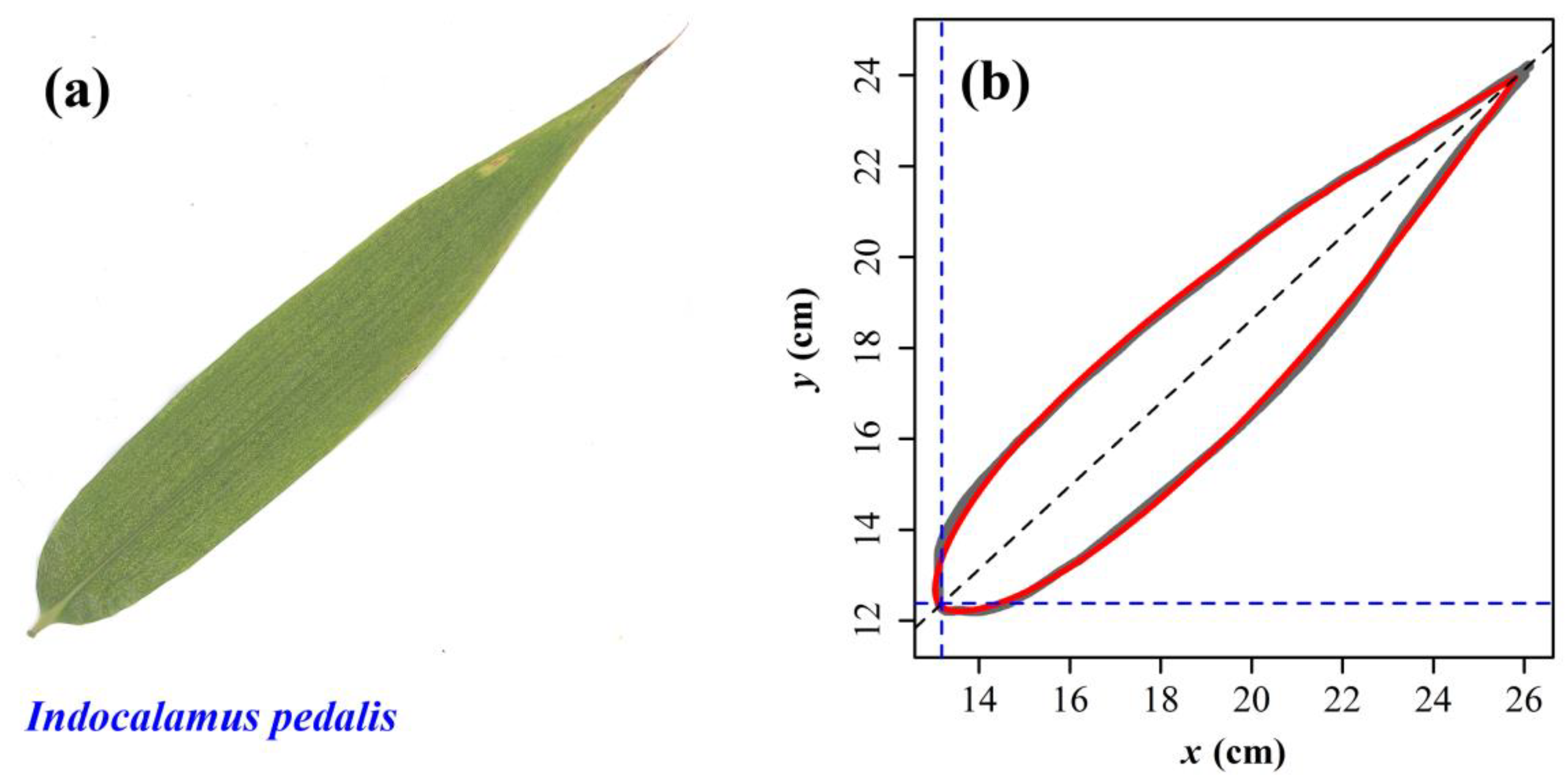
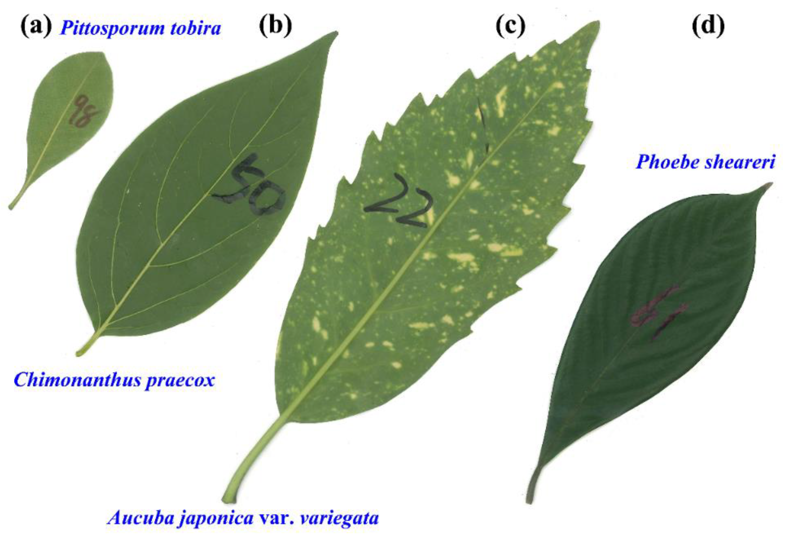
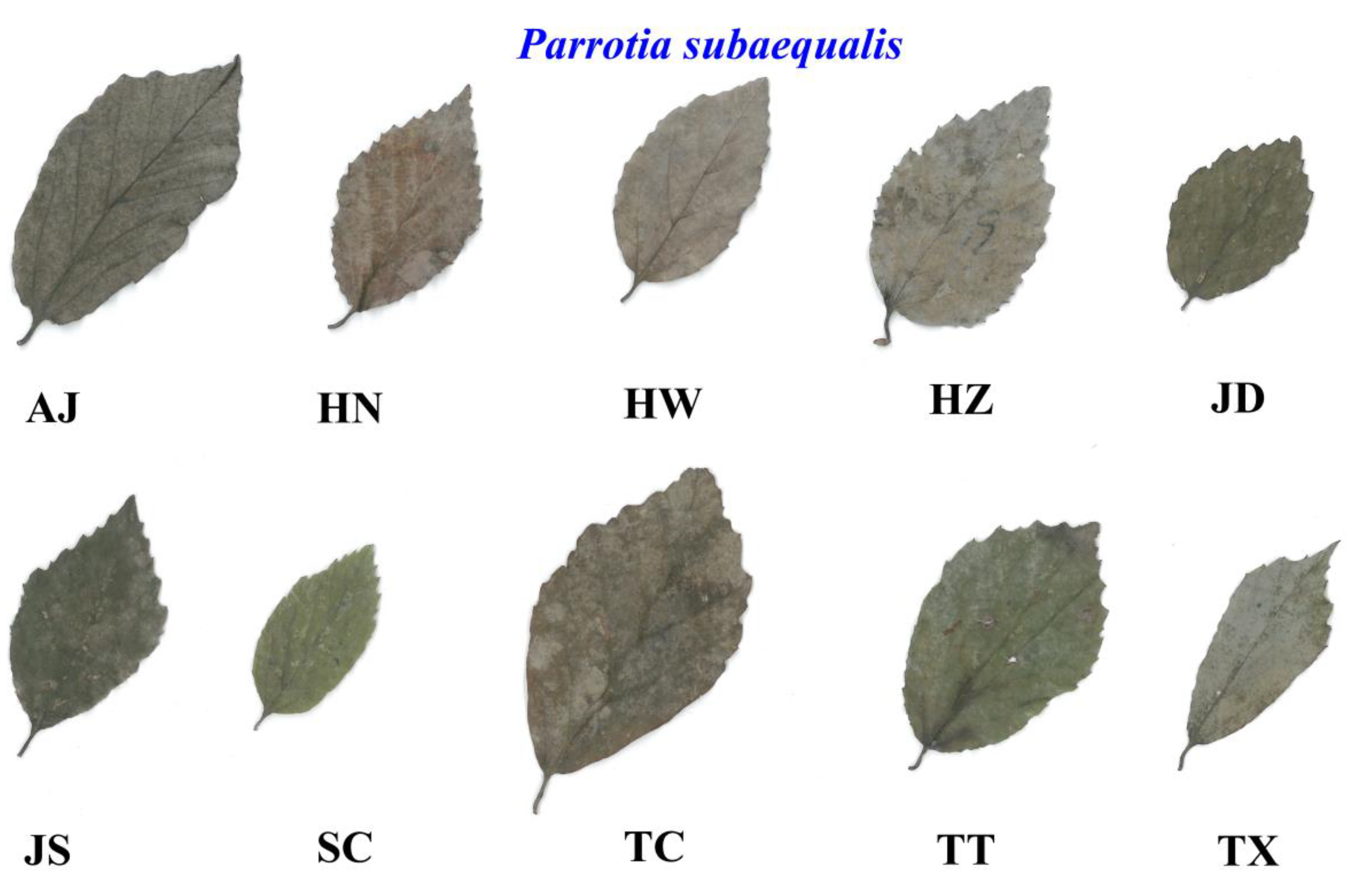
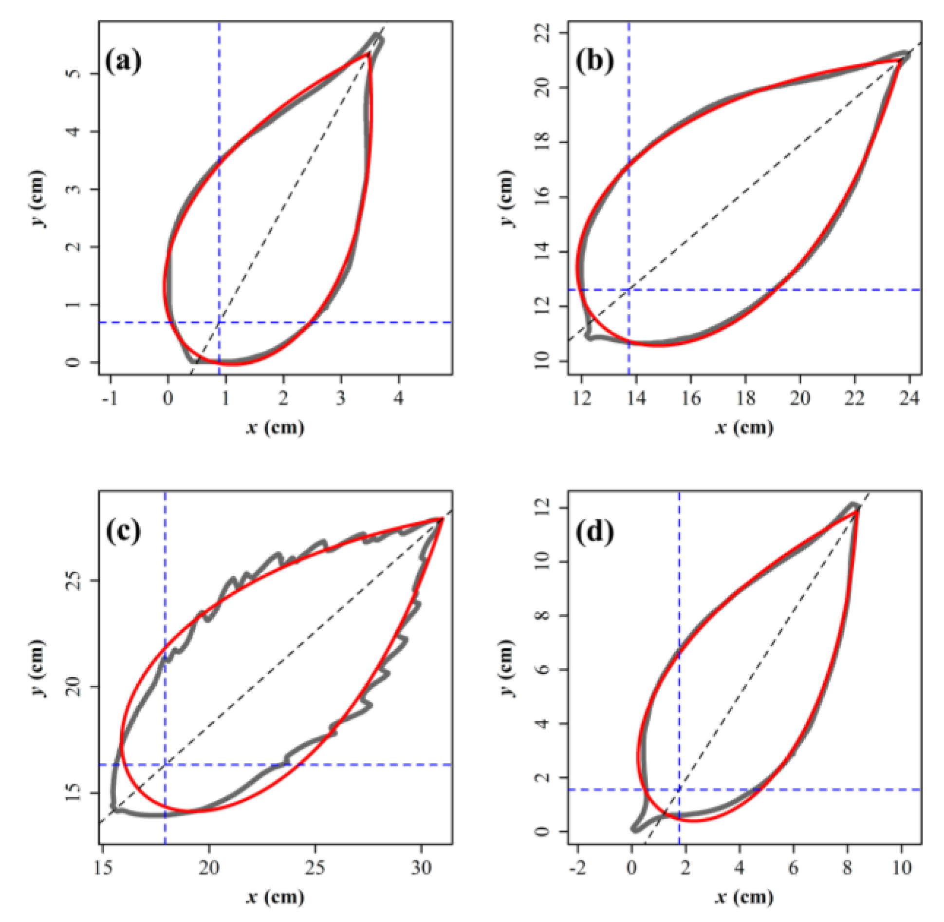
2.1. Materials

Nine datasets are available: (1) 42 species of bamboos were randomly chosen, each species having about 30 ‘standard’ leaves whose length values approximate the medians calculated using 500 leaves for every bamboo species; (2) 4 species of bamboos from the same genus Indocalamus, each species having more than 100 leaves; (3) 193 leaves of Bambusa multiplex f. fernleaf (R. A. Young) T. P. Yi; (4) 209 leaves of Phyllostachys incarnata T. H. Wen; (5) 510 leaves of Pleioblastus chino (Franchet & Savatier) Makino; (6) 202 leaves of Pseudosasa amabilis (McClure) Keng f.; (7) 199 leaves of Sasaella kongosanensis ‘Aureostriatus’ (Nakai) Nakai ex Koidz; (8) 4 species of trees, among which one species has 75 leaves and the others have ≥ 100 leaves; (9) 10 geographical populations of Parrotia subaequalis (Hung T. Chang) R. M. Hao & H. T. Wei, with each population having 30 leaves randomly chosen from the trees. Tables S1–S5 (see the online Supplementary Material S1) list the details of the Latin names of plants, collection times, locations, and number of leaves sampled. More species and experimental information can be found in Shi et al. [7,16] and Lin et al. [8,17]. Except for dataset 1, where the leaf lengths of the sampled leaves approximated their medians, the remaining leaves were randomly picked from the plants. Because the leaf shapes of all bamboos were similar, we show only the leaf shape of one species of bamboo (Figure 1a); Figure 2 shows the leaf shapes of four tree species; Figure 3 shows the leaf shapes of 10 geographical populations of P. subaequalis.

2.2. Models

The simplified Gielis equation can be used to depict the leaf shape of bamboos [6,7,8]:

$$r=\frac{l}{{\left(\left|\cos \frac{\phi }{4}\right|+\left|\sin \frac{\phi }{4}\right|\right)}^{1/n}}$$

(1)

where r represents the polar radius at polar angle φ; l and n are constants. For any point on the leaf edge, its x coordinate equals r cosφ, and its y coordinate equals r sinφ. Leaf length (L) equals r(0) + r(π), which can be written as:

$$L=\left(1+2^{-0.5/n}\right)l\iff l={\left(1+2^{-0.5/n}\right)}^{-1}L$$

(2)

In the first quadrant, the derivative of y with respect to φ can be expressed as:

$$\begin{array}{ll}\frac{dy}{d\phi }& =\frac{d\left(r\sin \phi \right)}{d\phi }\\ & =l\left[\cos \phi {\left(\cos \frac{\phi }{4}+\sin \frac{\phi }{4}\right)}^{-1/n}-\frac{\sin \phi }{4n}\left(\cos \frac{\phi }{4}-\sin \frac{\phi }{4}\right){\left(\cos \frac{\phi }{4}+\sin \frac{\phi }{4}\right)}^{-1/n-1}\right]\end{array}$$

(3)

When the line passing through the leaf apex and the leaf base is parallel to the x-axis, dy/dφ = 0. Perpendicular to this, the line segment passing through these two points on the leaf edge is vertical, and its length (representing leaf width) is maximal. In this case, we have:

$$n=\frac{\tan {\phi }_w}{4}\frac{\cos \frac{{\phi }_w}{4}-\sin \frac{{\phi }_w}{4}}{\cos \frac{{\phi }_w}{4}+\sin \frac{{\phi }_w}{4}}$$

(4)

The subscript w of φ represents the special value of φ at the point where leaf width is maximal. On the basis of Equations (1) and (2), leaf width (W) equals:

$$\begin{array}{ll}W& =2\sin {\phi }_w{r}_w\\ & =2\sin {\phi }_w\frac{L}{\left(1+2^{-0.5/n}\right){\left(\cos \frac{{\phi }_w}{4}+\sin \frac{{\phi }_w}{4}\right)}^{1/n}}\end{array}$$

(5)

There is no analytical solution for the parameter φ_w linked to leaf length and leaf width. However, a numerical solution for the parameter can be obtained. We can set a group of candidates of φ in small increments (e.g., 10⁻⁶) from 0 to π/2. Then, we calculate the approximate value of leaf width based on Equations (4) and (5) by minimizing the absolute value of the difference between the actual measured leaf width and the predicted values by Equation (5). Then, we can obtain the angle associated with the minimal absolute value of the differences, which is the numerical solution of φ_w. As a consequence, the parameter n can be obtained according to Equation (4), and then l_w can also be obtained according to Equation (2). The LA formula can be expressed as:

$$\begin{array}{ll}\mathrm{LA}& =\frac{1}{2}{\displaystyle {\int }_0^{2\pi }{r}^2}d\phi =\frac{1}{2}{\displaystyle {\int }_0^{2\pi }{l}^2}{\left(\left|\cos \frac{\phi }{4}\right|+\left|\sin \frac{\phi }{4}\right|\right)}^{-2/n}d\phi \\ & =f\left(l,n\right)=g\left(L,W\right)\end{array}$$

(6)

where f and g represent two different mathematical functions.

2.3. Statistical Analyses

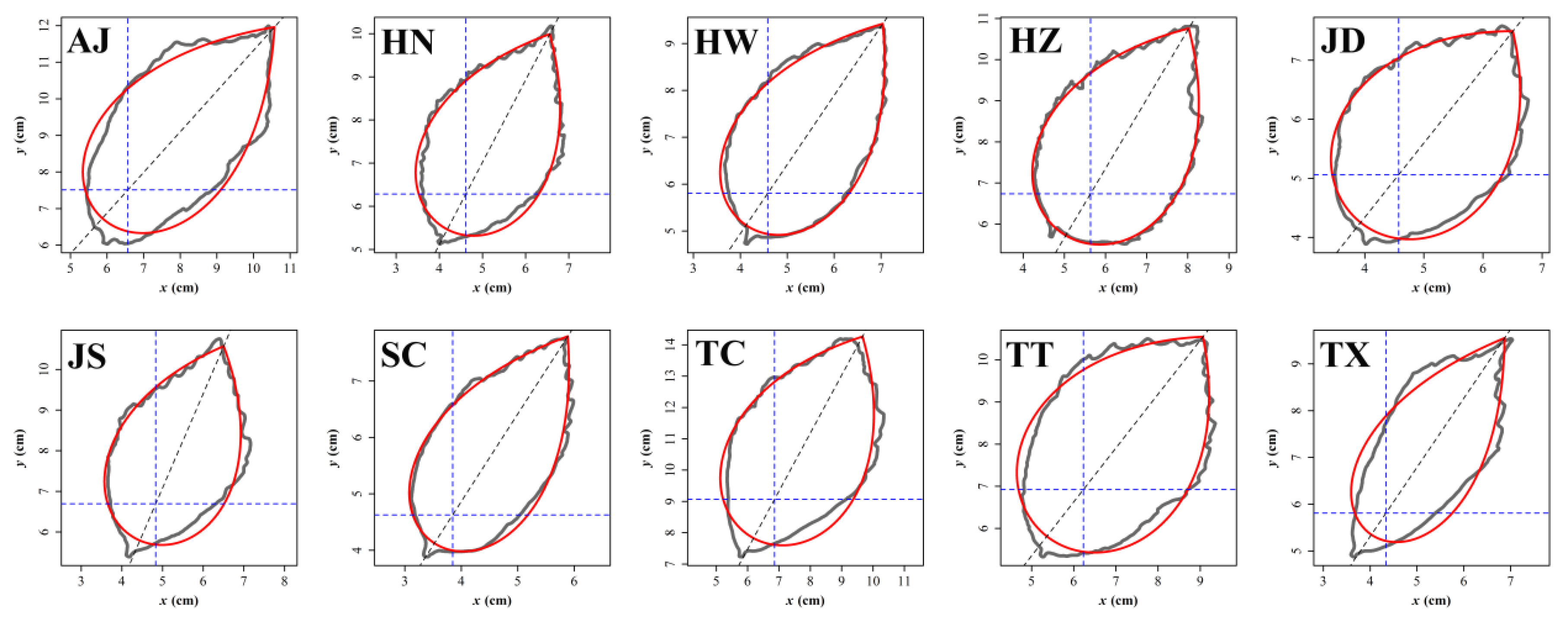
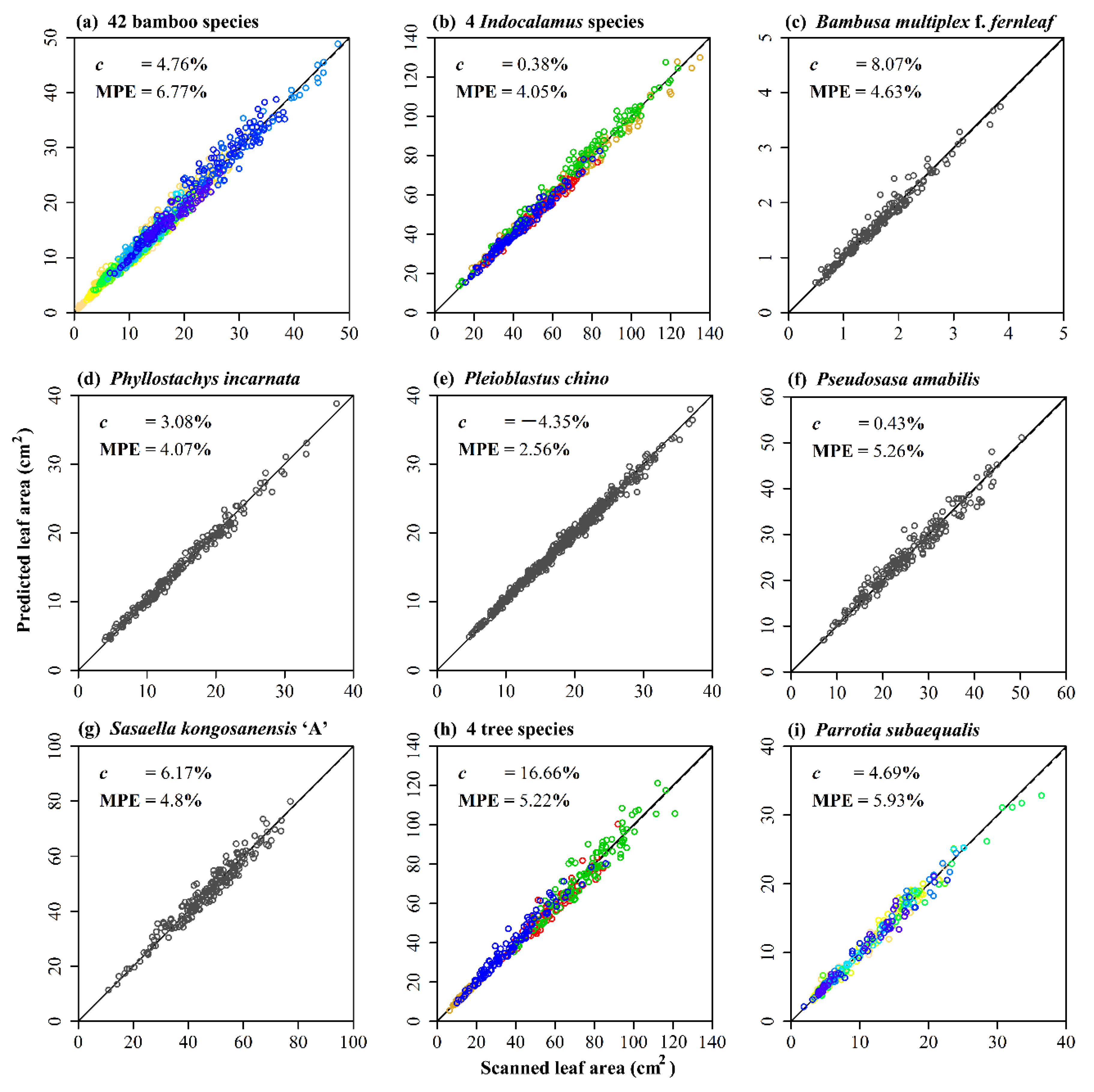
The leaves were scanned into black−white images in the bitmap format. The planar coordinates of the edge of any leaf were extracted using the revised version of the M-file developed by Shi et al. [18], which produces a CSV file (see the online Supplementary Materials S2 and S3). The planar coordinates were then further adjusted using the R script in the online Supplementary Materials S4–S6. The SGE was used to fit the leaf edge data by minimizing the residual sum of squares (RSS) between the actual and predicted polar radii. In this way, it could be evaluated whether the SGE describes the leaf edge well. We also developed R functions (see the online Supplementary Materials S4–S6 for details) for calculating the leaf area based on the measured leaf length and leaf width.

Because the leaves of some plants are very long and cause the leaf length predicted by the SGE to be smaller than the actual length, we set up a group of ratio (c) candidates from 0 to 0.2 with an increment of 0.0001. For P. chino, we used a group of negative ratio candidates from −0.2 to 0 with an increment of 0.0001. We referred to c as the floating ratio in leaf length. Using the measured leaf width and the product of the measured leaf length and (1 − c), LA values could be predicted. That is:

$$\mathrm{LA}=g\left[\left(1-c\right)L,W\right]$$

(7)

Note: the g function’s expression did not change, but the first independent variable changed from L to (1 − c) L.

RSS was used as the target function of optimization to obtain the estimate of c. To measure and compare the prediction errors among different plants, the percent error (PE) was used:

$$\mathrm{PE}=\left|\frac{\mathrm{LA}-\widehat{\mathrm{LA}}}{\mathrm{LA}}\right|\times 100\%$$

(8)

where LA represents the scanned leaf area, and $\widehat{\mathrm{LA}}$ represents the calculated leaf area using Equation (7). If there are q leaves for a species, we can calculate the mean percent error MPE = ${{\displaystyle \sum }}_{i=1}^q{\mathrm{PE}}_i/q$, which directly compares the model’s validity for different species. Plotting the predicted LA against the scanned LA with the straight line y = x intuitively exhibits the goodness of fit. In addition, a linear regression between scanned LA and predicted LA checks whether the linear regression approximates the straight line y = x and tests whether the intercept of the straight line is significant.

3. Results

Figure 1b shows the result of using the SGE to fit the leaf shape of a bamboo species. The withered part of the leaf apex (Figure 1a) was removed while making the black−white image, because this part does not essentially participate in photosynthesis. Figure 4 shows the fitted results for the leaf shapes of four species of trees. For P. tobira and P. sheareri, we interchanged the positions of leaf apex and leaf base to enhance the goodness of fit. In this case, the leaf apex was actually nearer to the origin than to the leaf base (Figure 4a,d). For the four tree species, the leaf widths predicted by the SGE all approximated their actual values, although the predicted leaf lengths were always smaller than their actual values. For A. japonica var. variegata, there was a large prediction error in the leaf shape. Figure 5 shows the fitted results of the leaf shapes of 10 geographical populations of P. subaequalis. The SGE was generally good for describing the leaf shapes of these 10 populations, except for a relative large deviation for the populations ‘AJ’ and ‘TX’. By reversing the positions of the leaf apex and leaf base, we should have obtained better results in leaf−shape fitting for some leaves. However, there was also a certain amount of variation in leaf shape within the same population. Sometimes, the used northeastern directional arrangement from leaf base to leaf apex on the image could provide a better fit than the southwestern directional arrangement, but sometimes the latter was better. In the former case, all leaves for the 10 geographical populations were arranged in a northeastern direction before carrying out the SGE fitting.

We further evaluated the model’s validity by comparing the scanned and predicted leaf areas based on the SGE (Figure 6a–i). For standard leaves of 42 bamboo species, the theoretical leaf length (predicted by the SGE) was estimated to be 4.76% smaller than the actual value (represented by the scanned leaf length), and the corresponding MPE between scanned and predicted LA was 6.77% (Figure 6a). The intercept of the linear regression equation was equal to 0.0969 and statistically insignificant (p = 0.139). For four bamboo species of Indocalamus, the theoretical leaf length was predicted to be 0.38% smaller than the actual value, and the corresponding MPE was lower than 5% (Figure 6b). The intercept of the linear regression equation was equal to 0.9602 and statistically significant (p < 0.01). For B. multiplex f. fernleaf, the theoretical leaf length was predicted to be 8.07% smaller than the actual value, and the corresponding MPE was lower than 5% (Figure 6c). The intercept of the linear regression equation was equal to 0.0512 and statistically significant (p < 0.01). For Ph. incarnata, the theoretical leaf length was predicted to be 3.08% smaller than the actual value, and the corresponding MPE was lower than 5% (Figure 6d). The intercept of linear regression was equal to 0.5683 and statistically significant (p < 0.01). For P. chino, the theoretical leaf length was predicted to be 4.35% greater than the actual value, and the corresponding MPE was lower than 3% (Figure 6e). The intercept of linear regression was equal to 0.6470 and statistically significant (p < 0.01). For P. amabilis, the theoretical leaf length was predicted to be 0.43% smaller than the actual value, and the corresponding MPE was slightly higher than 5% (Figure 6f). The intercept of linear regression was equal to 1.4839 and statistically significant (p < 0.01). For S. kongosanensis ‘Aureostriatus’, the theoretical leaf length was predicted to be 6.17% smaller than the actual value, and the corresponding MPE was lower than 5% (Figure 6g). The intercept of the linear regression equation was equal to 2.1435 and statistically significant (p < 0.01). For four species of trees, the theoretical leaf length was predicted to be 16.66% smaller than the actual value, and the corresponding MPE was slightly higher than 5% (Figure 6h). The intercept of the linear regression equation was equal to 0.1672 and statistically insignificant (p = 0.644). For the 10 geographical populations of P. subaequalis, the theoretical leaf length was predicted to be 4.69% smaller than the actual value, and the corresponding MPE was approximately 6% (Figure 6i). The intercept of the linear regression equation was equal to 0.3164 and statistically significant (p < 0.01).

Although the majority of intercepts were statistically significant, the intercepts could be regarded as ‘zero’ relative to the upper bounds of the scanned leaf area (the ratios of the intercept’s estimate to the maximum LA were all less than 0.5% of LA).

4. Discussion

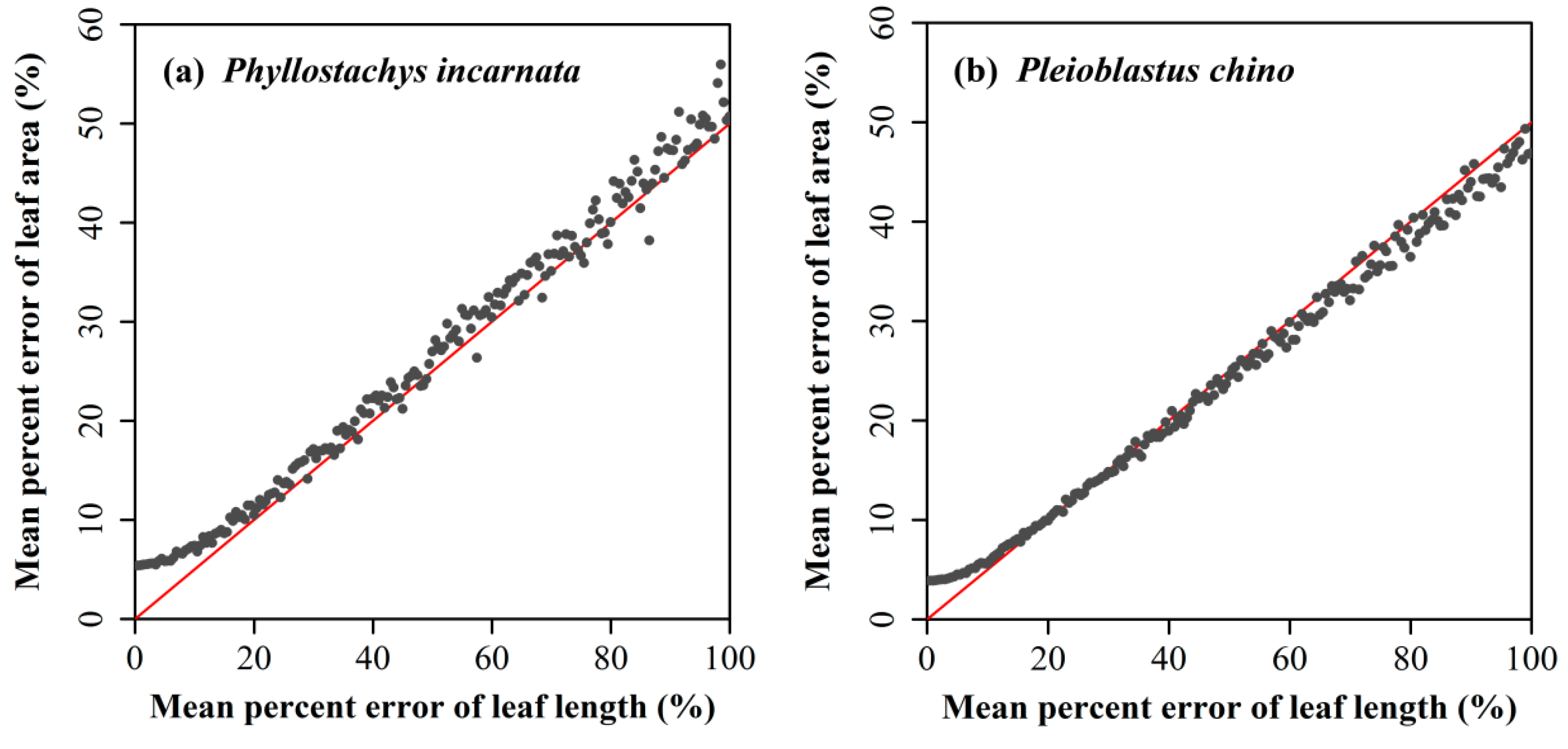
4.1. Influence of the Prediction Error in Leaf Length on Computing the Leaf Area

In our experiment, the predicted leaf width appeared to approximate the actual value; however, for all plants, except for P. chino that has an unusual long leaf relative to other bamboo species, the predicted leaf lengths by the SGE were lower than the actual (‘scanned’) leaf lengths. The majority of the estimates of the floating ratios (c) in leaf length were larger than 0. Interestingly, although there were different degrees of deviation between the predicted and the scanned leaf lengths (c ranging from 0% to 17%), the mean percent errors in LA were all lower than 7%. In order to explain this, we used the datasets of Ph. incarnata and P. chino (i.e., datasets 4 and 5). A group of assumed mean percent errors of leaf length (MPEL) from 0.5% to 100% in 0.5% increments was generated. For each assumed MPEL, the leaf length data were reassigned by a value randomly chosen in an interval of (L(1 − MPEL), L(1 + MPEL)), where L represents the original scanned leaf length. We calculated the mean percent error of leaf area (MPEA) based on the reassigned length data. Then, the influence of MPEL on MPEA could be found (Figure 7). When MPEL was lower than 20%, the MPEA was lower than 10%. When MPEL exceeded 20%, MPEL was twice as big as MPEA. That means that the prediction error in leaf area was only 1/2 of that in leaf length. Although the influence of MPEL on MPEA can be altered by using different values for different species (we do not show the results using other species here), the overall trend of MPEA versus MPEL was relatively stable: below a critical value of MPEL, the mean prediction error in leaf area increased slowly; above this critical value, MPEA increased linearly and was approximately half the size of MPEL.

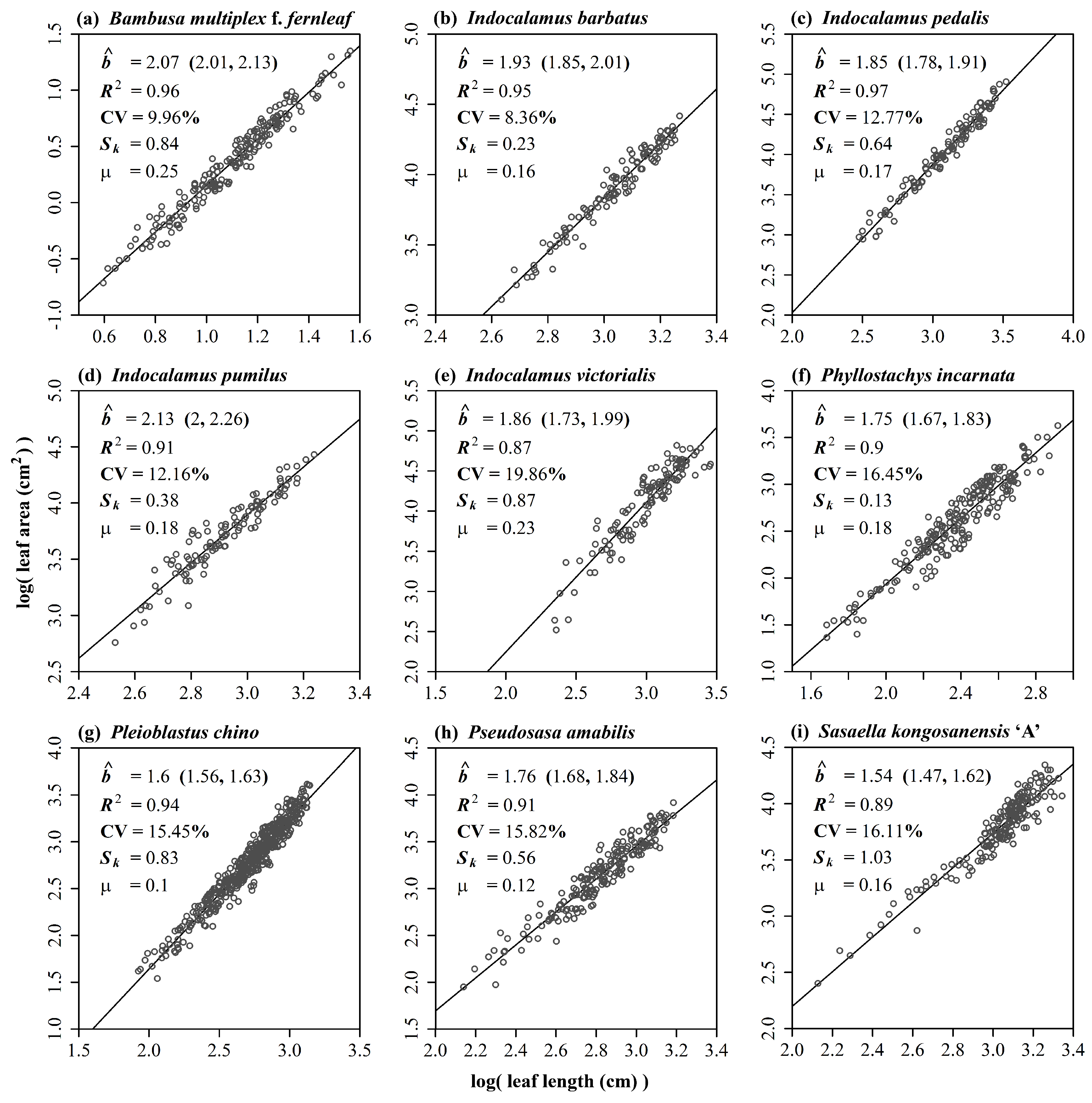
4.2. Beyond the Power Law between Leaf Length and Leaf Area

Thompson [19] provided a principle of similarity: the area is proportional to the length to the power 2, and the weight is proportional to the area to the power 3/2 on the condition that the density is uniform. The principle of similarity has been confirmed in animals, especially fishes [20,21]. However, for leaves, the scaling exponent between leaf weight and leaf area is lower than 3/2 [2,17]. There are some studies that have confirmed the principle of similarity in the scaling relationship between leaf area and leaf length [22]. However, using leaf length, large deviations of the predicted log(LA) from the observed log(LA) have been found. Thus far, there have been no relevant studies to explain this disagreement. In our recent study, we demonstrated that LA based on the SGE is a function of leaf length to the power of 2 under the assumption that parameter n in the SGE is approximately a constant for all the leaves of the same species [17]. However, every leaf actually has a different n value for the same bamboo species [7,8]. From Equations (4) and (5), it is apparent that φ_w can be treated as a function of the ratio of leaf width to leaf length (i.e., the W/L ratio). Then, n is actually a function of W/L, on the basis of Equation (4). In this case, whether there is a ‘power of 2′ law between LA and leaf length might mainly rely on the shape of the distribution of n or that of the ratio of W to L. If the coefficient of variation of the ratios (CV = σ/μ, where μ and σ represent the mean and the standard deviation of the leaf width/length ratios, respectively) is very low, which means that the distribution curve of the leaf width/length ratios is narrow, we would expect that the estimate of the scaling exponent between leaf length and leaf area approximates 2 (Figure 8a,b). In this case, n values for different leaves vary in a small range. We also checked whether the extent of skewness of the distribution of the leaf width/length ratios can affect the estimate of slope. Skewness (S_k) of the leaf width/length ratios was measured by the following equation:

$$S_k=E\left[{\left(\frac{x-\mu }{\mathsf{\sigma }}\right)}^3\right]$$

(9)

where E represents expectation, and x represents the vector of leaf width/length ratio. The smaller the absolute value of skewness, the more symmetrical the distribution curve of the ratios. For four bamboo species of Indocalamus, a lower skewness corresponded to an estimate of slope (namely, the power) that approximated 2 (Figure 8b). However, a larger skewness also associated with such an estimate (Figure 8a). This might be caused by a lower CV. Thus, we can draw the following conclusions: if the coefficient of variation and skewness of the leaf width/length ratios were both low, the estimate of the scaling exponent between leaf length and leaf area would approximate 2; if these two indicators were both high, the estimate would largely deviate from 2; on the condition that the values of one indicator were the same or approximately so, a lower value of the other indicator would correspond to an estimate that approximates 2 (Figure 8). Note that we did not use the pooled leaf length−area data from different species or different geographical populations here. Overall, whether or not the principle of similarity of Thompson [19] about the area–length scaling relationship for leaves can hold relies mainly on the distribution of leaf width/length ratios. In fact, when we examined this conclusion using some plants with sagittate leaf shape (e.g., the analogous triangle-like Polygonum perfoliatum L. or Oxalis triangularis A.St.-Hil.), their LA could be approximately calculated by the triangular area formula: one-half the product of base and height, where base is actual leaf width, and height is leaf length. In this case, whether the leaf area is proportional to the leaf length to the power of 2 apparently also relies on the distribution of the leaf width/length ratios (or the distributions of the apex angle of the triangle). When the apex angle varies in a small range, the area will change with the length to the power of 2.

4.3. Comparison between a Non-Parametric Model and the Gielis Equation

Our method requires a training set to obtain the estimate of the floating ratio in leaf length (i.e., c). However, there are existing non-parametric fitting methods, such as local regression, generalized additive model (GAM), kernel estimation, and neural network algorithm [23]. These techniques essentially let the (training) data ‘speak’. If a training set of leaf length and leaf width exists, the non-parametric models usually can fit the training set very well. If the predicted results using the GAM and SGE methods approximate those for the test set, it indicates that the SGE is a good candidate parametric model. To compare them, we used three datasets of bamboos (datasets 4–6) with different floating ratios, i.e., 3.08%, −4.35%, and 0.43% (Figure 6d–f). The golden ratio was used to divide a dataset into two parts: training set and test set [24]. In practice, we hoped to use a small number of leaves to obtain the estimates of floating ratio in the SGE and fitted results in the GAM. Thus, 38.2% of the dataset was randomly sampled as the training set, and the remaining 61.8% of the dataset was used as the test set. On the basis of the leaf length, leaf width, and scanned LA data in the training set, the floating ratio (c) in leaf length was obtained by minimizing the RSS between the scanned and predicted LAs using the SGE. Then, we calculated the RSS between the scanned and the predicted LAs in the test set. A simple GAM was used to predict LA:

LA = s(L) + s(W)

(10)

where s represents the smooth function in the GAM. Also, 38.2% of the dataset (including the data of leaf length, width, and corresponding area) was randomly sampled as the training set. Then, we used it to predict the LAs of the test set. Because the test sets for the two methods came from the same species, the mean percent error was not used. In this case, it was unnecessary to standardize the data for interspecific comparison. RSS or root mean squared error (RMSE, the square root of RSS/N, where N represents data length) was sufficient as the indicator of goodness of fit. The RMSE from the GAM prediction was calculated to compare it with the SGE prediction, because RMSE can be regarded as the ‘average absolute deviation’ of the observed LA from the predicted LAs. For datasets 4–6, 3000 random sampling replications were carried out. Figure 9 shows the results of the comparison of the two methods based on the three datasets. For three datasets, using 3000 bootstrap replications, the 95% confidence interval of the differences between RMSE_SGE replicates and RMSE_GAM replicates included zero (Figure 9g–i), which demonstrates that there was no significant difference between the SGE and GAM [25,26]. That is, the SGE is a parametric model with general applicability for describing the leaf shape of many plants. If there was a small variation in leaf length (i.e., a small MPEL), the difference in RMSE between the two methods would be smaller (Figure 9d,f); if the MPEL was large, the RMSE predicted by the SGE would be slightly higher than that predicted by the GAM (Figure 9e). It is necessary to point out that the RMSE values using the GAM to fit the training set were all approximately zero, but the RMSE values using the above GAM to fit the test set were substantially larger than the former ones (Figure 9a versus Figure 9d, Figure 9b versus Figure 9e, Figure 9c versus Figure 9f). The non-parametric fitting method might have led to over-fitting to a certain extent (see the RMSE using the GAM in Figure 9a–c).

5. Conclusions

In summary, the simplified Gielis equation can be used to describe the leaf shapes of many plants. Its prediction of leaf width usually approximates the actual value of leaf width, whereas its prediction of leaf length is mostly lower than the observed value of leaf length. We introduced a floating ratio in leaf length and found that the predicted areas using the SGE fit the observed leaf areas well for nine datasets including 53 species (which included 48 bamboo plants, 5 woody plants, and 10 geographical populations of a woody plant, totaling 3310 leaves). The mean percent errors of LA prediction for all studied plants were lower than 7%, among which, the mean percent errors for most bamboo plants were lower than 5%. We found that below a critical value of percent error in leaf length, the MPEA increased slowly with increases in the MPEL; after this critical value, the MPEA increased linearly with 1/2 MPEL. However, in practice, the estimate of MPEL might not exceed that critical value. Relative to the GAM, the LAs predicted by the SGE had a larger coefficient of variation in the goodness of fit if the percent error in leaf length was large; however, there was no significant difference in RMSE between the GAM and the SGE for the three datasets. We have grounds for believing that the SGE has a wide applicability in describing the leaf area for many plants with elliptical, heart-shaped, or linear leaves. It merits further investigation in other plants.

References

1. Jurik, T.W. Temporal and spatial patterns of specific leaf weight in successional northern hardwood trees species. Am. J. Bot. 1986, 73, 1083–1092. [Google Scholar] [CrossRef]
2. Milla, R.; Reich, P.B. The scaling of leaf area and mass: The cost of light interception increases with leaf size. Proc. R. Soc. Biol. Sci. 2007, 274, 2109–2114. [Google Scholar] [CrossRef] [PubMed]
3. Schrader, J.; Pillar, G. Leaf-IT: An Android application form measuring leaf area. Ecol. Evol. 2017, 7, 9731–9738. [Google Scholar] [CrossRef] [PubMed]
4. Dornbusch, T.; Watt, J.; Baccar, R.; Fournier, C.; Andrieu, B. A comparative analysis of leaf shape of wheat, barley and maize using an empirical shape model. Ann. Bot. 2011, 107, 865–873. [Google Scholar] [CrossRef] [PubMed]
5. Gielis, J. Inventing the Circle: The Geometry of Nature; Geniaal Press: Antwerpen, Belgium, 2003. [Google Scholar]
6. Gielis, J. The Geometrical Beauty of Plants; Atlantis Press: Paris, France, 2007. [Google Scholar]
7. Shi, P.; Xu, Q.; Sandhu, H.S.; Gielis, J.; Ding, Y.; Li, H.; Dong, X. Comparison of dwarf bamboos (Indocalamus sp.) leaf parameters to determine relationship between spatial density of plants and total leaf area per plant. Ecol. Evol. 2015, 5, 4578–4589. [Google Scholar] [CrossRef] [PubMed]
8. Lin, S.; Zhang, L.; Reddy, G.V.P.; Hui, C.; Gielis, J.; Ding, Y.; Shi, P. A geometrical model for testing bilateral symmetry of bamboo leaf with a simplified Gielis equation. Ecol. Evol. 2016, 6, 6798–6806. [Google Scholar] [CrossRef] [PubMed] [Green Version]
9. Nicotra, A.B.; Leigh, A.; Boyce, C.K.; Jones, C.S.; Niklas, K.J.; Royer, D.L.; Tsukaya, H. The evolution and functional significance of leaf shape in the angiosperms. Funct. Plant Biol. 2011, 38, 535–552. [Google Scholar] [CrossRef]
10. Jones, C.S.; Bakker, F.T.; Schlichting, C.D.; Nicotra, A.B. Leaf shape evolution in the South African genus Pelargonium L’ Hér. (Geraniaceae). Evolution 2008, 63, 479–497. [Google Scholar] [CrossRef] [PubMed]
11. Runions, A.; Fuhrer, M.; Lane, B.; Federl, P.; Rolland-Lagan, A.-G.; Prusinkiewicz, P. Modeling and visualization of leaf venation patterns. ACM Trans. Gr. 2005, 24, 702–711. [Google Scholar] [CrossRef]
12. Runions, A.; Tsiantis, M.; Prusinkiewicz, P. A common developmental program can produce diverse leaf shapes. New Phytol. 2017, 216, 401–418. [Google Scholar] [CrossRef] [PubMed] [Green Version]
13. Brodribb, T.J.; Feild, T.S.; Jordan, G.J. Leaf maximum photosynthetic rate and venation are linked by hydraulics. Plant Physiol. 2007, 144, 1890–1898. [Google Scholar] [CrossRef] [PubMed]
14. Price, C.A.; Symonova, O.; Mileyko, Y.; Hilley, T.; Weitz, J.S. Leaf extraction and analysis framework graphical user interface: Segmenting and analyzing the structure of leaf veins and areoles. Plant Physiol. 2011, 155, 236–245. [Google Scholar] [CrossRef] [PubMed]
15. Hastie, T.; Tibshirani, R. Generalized Additive Models; Chapman and Hall: London, UK, 1990. [Google Scholar]
16. Shi, P.; Zheng, X.; Ratkowsky, D.A.; Li, Y.; Wang, P.; Cheng, L. A simple method for measuring the bilateral symmetry of leaves. Symmetry 2018, 10, 118. [Google Scholar] [CrossRef]
17. Lin, S.; Shao, L.; Hui, C.; Song, Y.; Reddy, G.V.P.; Gielis, J.; Li, F.; Ding, Y.; Wei, Q.; Shi, P. Why does not the leaf weight-area allometry of bamboos follow the 3/2-power law? Front. Plant Sci. 2018, 9, 583. [Google Scholar] [CrossRef] [PubMed]
18. Shi, P.; Huang, J.; Hui, C.; Grissino-Mayer, H.D.; Tardif, J.; Zhai, L.; Li, B. Capturing spiral radial growth of conifers using the super ellipse to model tree-ring geometric shape. Front. Plant Sci. 2015, 6, 856. [Google Scholar] [CrossRef] [PubMed]
19. Thompson, D.W. On Growth and Form; Cambridge University Press: London, UK, 1917. [Google Scholar]
20. O’Shea, B.; Mordue-Luntz, A.J.; Fryer, R.J.; Pert, C.C.; Bricknell, I.R. Determination of the surface area of a fish. J. Fish. Dis. 2006, 29, 437–440. [Google Scholar] [CrossRef] [PubMed]
21. Shi, P.; Ishikawa, T.; Sandhu, H.S.; Hui, C.; Chakraborty, A.; Jin, X.; Tachihara, K.; Li, B. On the 3/4-exponent von Bertalanffy equation for ontogenetic growth. Ecol. Model. 2014, 276, 23–28. [Google Scholar] [CrossRef]
22. Firman, D.M.; Allen, E.J. Estimating individual leaf area of potato from leaf length. J. Agric. Sci. 1989, 112, 425–426. [Google Scholar] [CrossRef]
23. Hastie, T.; Tibshirani, R.; Friedman, J. The Elements of Statistical Learning: Data Mining, Inference, and Prediction, 2nd ed.; Springer: Berlin, Germany, 2009. [Google Scholar]
24. Shi, P.; Chen, Z.; Reddy, G.V.P.; Hui, C.; Huang, J.; Xiao, M. Timing of cherry tree blooming: Contrasting effects of rising winter low temperatures and early spring temperatures. Agric. For. Meteorol. 2017, 240–241, 78–89. [Google Scholar] [CrossRef]
25. Efron, B.; Tibshirani, R.J. An Introduction to the Bootstrap; Chapman and Hall/CRC: New York, NY, USA, 1993. [Google Scholar]
26. Sandhu, H.S.; Shi, P.; Kuang, X.; Xue, F.; Ge, F. Applications of the bootstrap to insect physiology. Fla. Entomol. 2011, 94, 1036–1041. [Google Scholar] [CrossRef]
Figure 1. A leaf of one bamboo plant and fitted results using the simplified Gielis equation (SGE). (a) Scanned leaf image; (b) Observed and predicted leaf edge. The gray curve represents the scanned (observed) leaf edge, and the red curve represents the leaf edge predicted by the SGE.
Forests 09 00714 g001
Figure 2. Leaf examples of four tree species. (a) Pittosporum tobira (Thunberg) W. T. Aiton; (b) Chimonanthus praecox (Linnaeus) Link; (c) Aucuba japonica var. variegata Dombrain; (d) Phoebe sheareri (Hemsl.) Gamble.
Forests 09 00714 g002
Figure 3. Leaf examples of 10 geographical populations of Parrotia subaequalis in eastern China. The letters below the leaf photos represent the codes of the geographical populations. AJ: Anji, Zhejiang Province; HN: Xinyang, Henan Province; HW: Huangwei, Yuexi, Anhui Province; HZ: Changhua, Huangzhou, Zhejiang Province; JD: Jingde, Anhui Province; JS: Yixing, Jiangsu Province; SC: Shucheng, Anhui Province; TC: Tongcheng, Anhui Province; TT: Tiantangzhai, Jinzhai, Anhui Province; TX: Tianxia, Yuexi, Anhui Province.
Forests 09 00714 g003
Figure 4. Fitted results using the SGE for four tree species. Panels (ad) represent P. tobira, C. praecox, A. japonica var. variegata and P. sheareri, respectively. For every panel, the gray curve represents the scanned (observed) leaf edge, and the red curve represents the leaf edge predicted by the SGE. The leaves correspond to those in Figure 2.
Forests 09 00714 g004
Figure 5. Fitted results using the SGE for the 10 geographical populations of P. subaequalis. AJ: Anji, Zhejiang Province; HN: Xinyang, Henan Province; HW: Huangwei, Yuexi, Anhui Province; HZ: Changhua, Huangzhou, Zhejiang Province; JD: Jingde, Anhui Province; JS: Yixing, Jiangsu Province; SC: Shucheng, Anhui Province; TC: Tongcheng, Anhui Province; TT: Tiantangzhai, Jinzhai, Anhui Province; TX: Tianxia, Yuexi, Anhui Province. For every panel, the gray curve represents the scanned (observed) leaf edge, and the red curve represents the leaf edge predicted by the SGE. The leaves correspond to those in Figure 3.
Forests 09 00714 g005
Figure 6. Comparison between the scanned leaf area and the predicted leaf area based on leaf length and leaf width with an additional parameter, i.e., the floating ratio in leaf length (c). Panels (ai) represent the results of the comparison between the scanned and predicted leaf areas for the nine datasets (see 2.1 Materials for details), respectively. MPE denotes the mean percent error of leaf area. The solid line represents y = x, and the dashed line represents the regression line between the scanned and the predicted leaf areas. In each panel, the small open circles regardless of colors represent the planar coordinates consisting of the scanned leaf area (as the x-coordinate) and the predicted leaf area (as the y-coordinate). In panels (a,b,h), each color represents a species. However, the same colors in different panels do not represent the same species. In panel (i), different colors represent different geographical populations.
Forests 09 00714 g006
Figure 7. Effect of the mean percent error of leaf length on the mean percent error of leaf area based on the data of (a) Phyllostachys incarnata and (b) Pleioblastus chino (i.e., datasets 4 and 5). The grey solid circles represent the planar coordinates consisting of the mean percent error of leaf length (MPEL, as x-coordinate) and the mean percent error of leaf area (MPEA, as y-coordinate); the red straight line came from the equation y = 1/2 x. Take a grey solid circle whose MPEL equals 20% in panel (a), for example. There are 209 leaves for Ph. incarnata whose observations of leaf length and area are both known. For each leaf, we redefine its length by randomly choosing a value in the range (0.8 L, 1.2 L), where L denotes the actual observation of leaf length. Then we can calculate the predicted value of leaf area based on the simplified Gielis equation, and consequently we are able to calculate the percent error of leaf area for this leaf. Because there are 290 leaves, we can obtain the mean percent error of leaf area that is exactly the y-coordinate associated with MPEL = 20% (namely the x-coordinate).
Forests 09 00714 g007
Figure 8. Scaling relationship between leaf area and leaf length. (a) Bambusa multiplex f. fernleaf (R. A. Young) T. P. Yi; (b) Indocalamus barbatus McClure; (c) Indocalamus pedalis (Keng) P. C. Keng; (d) Indocalamus pumilus Q. H. Dai and C. F. Keng; (e) Indocalamus victorialis P. C. Keng; (f) Phyllostachys incarnata T. H. Wen; (g) Pleioblastus chino (Franchet & Savatier) Makino; (h) Pseudosasa amabilis (McClure) Keng f.; (i) Sasaella kongosanensis ‘Aureostriatus’ (Nakai) Nakai ex Koidz. The open circles represent observations, and the solid line represents the regression line between leaf area and leaf length. Here, b ^ represents the estimate of slope (i.e., the scaling exponent between leaf area and leaf length); R2 represents the coefficient of determination to reflect the goodness of fit; CV is the coefficient of variation of the ratios of leaf width to leaf length; Sk represents the skewness of the ratios; μ represents the mean of the ratios.
Forests 09 00714 g008
Figure 9. Comparison of the goodness of fit for two methods. Three datasets, each representing a species, were used. The GAM represents the generalized additive model, and the SGE represents the simplified Gielis equation. CV represents the coefficient of variation in root mean squared error (RMSE). To test whether there is a significant difference in RMSE between the two methods, 3000 partitionings of the dataset were carried out using the golden ratio (38.2% for the training set and 61.8% for the test set) for each species’ dataset. Boxplots were obtained, based on these 3000 partitionings. Panels (ac) represent the training sets, and panels (df) represent the test sets. Panels (gi) exhibit the distribution of the differences in RMSE between the two methods based on the test set. The 95% confidence interval (CI) for each panel includes 0, which means that there was no significant difference in the goodness of fit between the two methods in predicting the leaf areas of the test set (see ref. [26]). However, there was an apparent significant difference in RMSE between the two methods based on the training set. The vertical blue dashed line represents the mean of the differences, and the two vertical gray dashed lines represent the 95% CI of the difference.
Forests 09 00714 g009