Article

How to Calibrate Historical Aerial Photographs: A Change Analysis of Naturally Dynamic Boreal Forest Landscapes

1
Department of Forest Sciences, University of Helsinki, P.O. Box 27, FI-00014 Helsinki, Finland
2
Research Unit of Mathematical Sciences, University of Oulu, P.O. Box 8000, FI-90014 Oulu, Finland
*
Author to whom correspondence should be addressed.
Forests 2018, 9(10), 631; https://doi.org/10.3390/f9100631
Submission received: 30 August 2018 / Revised: 6 October 2018 / Accepted: 9 October 2018 / Published: 11 October 2018
(This article belongs to the Special Issue Forest Landscape Ecology: Linking Past, Present, and Future Data)

Abstract

:
Time series of repeat aerial photographs currently span decades in many regions. However, the lack of calibration data limits their use in forest change analysis. We propose an approach where we combine repeat aerial photography, tree-ring reconstructions, and Bayesian inference to study changes in forests. Using stereopairs of aerial photographs from five boreal forest landscapes, we visually interpreted canopy cover in contiguous 0.1-ha cells at three time points during 1959–2011. We used tree-ring measurements to produce calibration data for the interpretation, and to quantify the bias and error associated with the interpretation. Then, we discerned credible canopy cover changes from the interpretation error noise using Bayesian inference. We underestimated canopy cover using the historical low-quality photographs, and overestimated it using the recent high-quality photographs. Further, due to differences in tree species composition and canopy cover in the cells, the interpretation bias varied between the landscapes. In addition, the random interpretation error varied between and within the landscapes. Due to the varying bias and error, the magnitude of credibly detectable canopy cover change in the 0.1-ha cells depended on the studied time interval and landscape, ranging from −10 to −18 percentage points (decrease), and from +10 to +19 percentage points (increase). Hence, changes occurring at stand scales were detectable, but smaller scale changes could not be separated from the error noise. Besides the abrupt changes, also slow continuous canopy cover changes could be detected with the proposed approach. Given the wide availability of historical aerial photographs, the proposed approach can be applied for forest change analysis in biomes where tree-rings form, while accounting for the bias and error in aerial photo interpretation.

1. Introduction

Tree growth and senescence occur slowly but continuously over large areas in the boreal forests [1]. Additionally, disturbances cause abrupt changes to the structure of these forests [2,3]. Several approaches have been developed to study forest structural changes which occur at various temporal scales. These include permanent plot measurements, where the same stand is repeatedly measured (e.g., [4]). In seasonal climates, another option is tree-ring based reconstruction, where the information stored in tree rings is used to analyze forest dynamics (e.g., [5]). However, these approaches face practical limitations. Permanent plots are rare, and, due to the high amount of work required, dendrochronological reconstructions are limited to small scales. Therefore, novel approaches that capture both slow and abrupt changes in forest ecosystems are required to understand how forest structure changes in time.
Remote sensing provides records over large spatial extent even at remote locations. For example, the Landsat satellites provide observations on global coverage from the early 1970s onwards [6]. However, among remotely sensed records, aerial photographs span the longest time period and currently enable the fine-scale analysis of vegetation dynamics over decades in many locations of the world [7]. Accordingly, aerial photographs have been used to study spatial [8,9,10] and temporal [3,11,12] vegetation dynamics, even at the scale of an individual tree [13].
As with any measurements, data derived from aerial photographs contain bias (systematic error) and error (random variation) [14]. For example, georectification errors [15], the aerial photo scale, defined by the focal length of the camera and the altitude from where the photo was taken [9,16], the quality (e.g., contrast, haziness, and shadowiness) [17,18], and texture and grain size of the photograph [18,19], as well as subjectivity in manual feature quantification [20], potentially produce errors. Hence, data derived from aerial photographs cannot be used for change analysis without accounting for the bias and error in the data.
Further, specifically in forested landscapes, the size and shape of the interpreted object (e.g., variation in tree crown sizes or species composition [13,21,22]), canopy surface roughness [8], the canopy cover [9], and the off-nadir view of the trees [23] have been identified as major error sources. Due to the off-nadir view, the errors may also vary in different parts of the same aerial photograph [13]. Moreover, topographic variability may cause differences in photo quality and interpretation success, especially in rugged terrain [24].
In the analysis of aerial photographs, the sources of bias and error are numerous, but their effects are generally neglected [14]. These errors could be accounted for by, e.g., calibrating aerial photographs with field-measured ground truth values [21]. However, the historical aerial photographs often lack such accurate and spatially explicit ground-truth data [22].
Previous studies on forest structural changes have sought to complement aerial photo interpretation with tree-ring analyses (e.g., [25,26]). However, instead of comprehensive change analysis, such studies have mostly focused only on the abrupt changes, such as wind, insect of fire disturbances (e.g., [27,28]). As tree-ring increment expresses yearly tree growth, the ring widths can be used to reconstruct tree diameter at a particular time point. Given the decadal span of aerial photographs, this means that also the slow continuous forest structural changes could be studied combining aerial photo and tree-ring analyses.
In this paper, we present an approach for quantifying the visual interpretation bias and error for historical aerial photographs by using tree-ring based reconstructions of forest stand development. We interpreted canopy cover in five naturally dynamic boreal forest landscapes using 2 km × 2 km interpretation grids with 0.1-ha cell size. We used Bayesian inference to discern credible changes from the bias and error noise, and tested the applicability of the approach by analyzing forest structural change between three time points. Specifically, we considered: (1) how bias and error in visual interpretation differ between aerial photographs of varying quality, and among the studied landscapes; and (2) what magnitude of forest structural changes can be detected with the approach.

2. Material and Methods

2.1. Study Area

We tested our approach at five naturally dynamic forest landscapes (2 km × 2 km) in two boreal regions: northeastern Finland (67°44′ N, 29°33′ E) and the North Shore region in Quebec, eastern Canada (49°38′ N, 67°55′ W). In Finland, we examined two landscapes in Värriö Strict Nature Reserve (Hirvaskangas and Pommituskukkulat), and a third landscape in Maltio Strict Nature Reserve (Hongikkovaara). In Quebec, we studied two landscapes, Lac Dionne and Pistuacanis.
The landscapes are mosaics of mineral soil forests, waterbodies, and forested and open peatlands. Soils are mostly undifferentiated glacial tills, topographical variation is gentle, and the low mountain fells have treeless upper slopes in northeastern Finland. Here, the elevation of the studied region ranges between 200 and 500 m above sea level (asl). Slopes vary from low to moderate in the North Shore region of Quebec. Undifferentiated glacial tills are common on the gentle slopes and depressions, as are glaciofluvial sand deposits in valley floors and rocky outcrops on slopes and summits [29]. Here, the elevation of the studied region ranges from 300 to 500 m asl. The mean annual temperature in the study region of northeastern Finland is −0.9 °C. The mean temperatures for the coldest (January) and warmest (July) months are −12.7 °C and +13.1 °C, respectively. The average annual precipitation sum is 570 mm. The mean annual temperature in the North Shore region is +0.3 °C. The mean temperatures for the coldest (January) and warmest (July) months are −17.5 °C and +14.2 °C, respectively. Average annual precipitation is 1100 mm (climate data are averages from years 1970–2000 [30]).
We tested the applicability of the approach in landscapes dominated by different tree species, and of varying tree cover. Pure Pinus sylvestris (L.) stands (proportion of P. sylvestris >75%) dominate Hirvaskangas landscape. Picea abies (L.) Karst. and Betula pubescens (Ehrh.) dominate the Pommituskukkulat landscape. In Hongikkovaara landscape, pure P. sylvestris stands and mixed P. sylvestris/P. abies stands prevail. Picea mariana (Mill.) dominates the Lac Dionne landscape and Abies balsamea (L.) Mill. the Pistuacanis landscape. Betula papyrifera (Marshall) occurs in both Quebecois landscapes.
Two regions with markedly different disturbance regimes were studied to test the functionality of the approach in change detection in different forest environments. In the Finnish region, forest fires were common prior to the 20th century, especially surface fires in the xeric P. sylvestris-dominated forests. The fire influence is visible in the age structure of the P. sylvestris-dominated areas, and as a high proportion of post-fire B. pubescens in the mesic areas [31]. In the absence of fire, the stands are influenced by gap dynamics, punctuated infrequently by storms felling trees over large areas [1].
In the Quebec study region, forests experience periodic spruce budworm, Choristoneura fumiferana (Clem.) outbreaks, to which A. balsamea is especially susceptible [32]. There is an ongoing outbreak in the North Shore region that began ca. 2006 [33]. The previous severe outbreak occurred from the 1970s to the mid-1980s [28]. Between outbreaks, gap dynamics drives the old-growth stands [2]. The Lac Dionne landscape burnt in 1810, while no fires occurred in Pistuacanis during the last 200 years [34].

2.2. Aerial Photographs and Their Orientation

We used canopy cover as a surrogate measure to quantify forest structural change over the past decades. We visually interpreted canopy cover using stereopairs of recent and two historical aerial photographs in each of the five study landscapes (Table 1). Henceforth, we call the photographs as the newest, middlemost and oldest photograph, and the time interval between the oldest and the middlemost photograph as the first study interval, the time interval between the middlemost and the newest photograph as the second study interval, and the time interval between the oldest and the newest photograph as the whole study interval.
The exact time span covered differed among the landscapes (Table 1), and the photo years depended on the availability of the photographs for each landscape. For the oldest photographs, we selected the oldest digitized photographs available for each landscape (varied between 1959 and 1972). For the middlemost photographs, for some landscapes several alternatives were available and we chose the ones with the best quality and stereo-cover over the landscape. For the newest photographs, we chose the most recent photographs available at the time of the fieldwork. The oldest photographs were panchromatic, and the others false-color.
Accurate solution of the exterior orientation of all photographs in a coordinate system that remains constant over time is required for precise retrospective photogrammetric measurements. Here, this was done using aerial triangulation. Normally, aerial triangulation relies on ground control points, which are often lacking from historical photographs. We circumvented the lack of ground control points by using the direct sensor orientation to solve the exterior orientation of the newest photographs that was delivered with this exterior orientation data, and the multitemporal tie points to bring the historical photographs to the same coordinate system with the newest photographs [34].
The newest photographs for all landscapes, the oldest photographs for Quebec, and the middlemost photographs for Pistuacanis were accompanied by exterior orientation parameters (projection center coordinates x, y, z, and the three camera rotation angles ω, φ, and κ). For the middlemost photographs in Pommituskukkulat and Hongikkovaara, camera calibration certificates were available, and contained information on the calibrated camera constant (i.e. the focal length or principal distance), location of the principal point in the fiducial coordinate system, and lens distortions. For the middlemost photographs in Hirvaskangas and Lac Dionne, and the oldest photographs in all the Finnish landscapes, only the calibrated camera constant was available. For those, the standard values for the camera type were used for the fiducial mark coordinates and the fiducial center position. Lens distortions were not corrected.
Due to the lack of ground-control points, we started out by measuring the coordinates for objects that were visible in the well-oriented new photographs, and on the photo to be oriented. These included large rocks, building corners, and bases of solitary trees. The z coordinate (elevation) for these points was derived from the digital elevation models (National Land Survey Finland, Ministère des Forêts, de la Faune et des Parcs du Québec). The photo orientation was done using the experimental software developed in [35], and ESPA Software (ESPA Systems Ltd., Espoo, Finland).

2.3. Visual Canopy Cover Interpretation

The first author visually interpreted canopy cover from the aerial photographs using a grid of 0.1 ha cells (31.62 m × 31.62 m, 4096 cells per grid), constructed with the Fishnet-tool in ArcGIS Desktop 9.3 (Environmental Systems Research Institute, Redlands, CA, USA). For the stereointerpretation, a grid needs information for elevation at grid nodes. This information was derived from the digital elevation model with 10 m horizontal resolution in Finland (National Land Survey Finland) and 20 m in Quebec (Ministère des Forêts, de la Faune et des Parcs du Québec). For each grid cell, canopy cover was estimated as the proportion of forest floor covered by the vertical projections of tree crowns. If a cell was not completely forested (e.g., waterbody or open peatland) at any time, it was excluded. In Pommituskukkulat, we also excluded cells overlapping or bordering a reindeer fence traversing the landscape. To reduce bias due to improving interpretation skill, we divided the interpretation grids into sixteen parts (256 cells each). Using these sub-grids, the newest photographs for each landscape were interpreted first in randomized order, and then the other photographs in randomized order. From the newest photographs, we also recorded the proportion of various tree species of the total canopy cover. We identified conifers to species level, but did not separate the deciduous trees. We performed the interpretation with EspaCity software (version 11.0.15306.1; ESPA Systems Ltd., Espoo, Finland), using a passive 3D monitor.

2.4. Field Data for the Calibration of the Canopy Cover Interpretation

We used field measurements and tree-ring data to obtain ground truth values (for interpretation calibration and the error distribution quantification) for the aerial photographs. To select the cells for field sampling, we first divided the interpretation grids into quadrants, and randomly selected 4 cells in each quadrant (16 per landscape). For logistic constraints, we only sampled 2–3 cells per quadrant in Quebec (9 cells per landscape). The purpose of this division was to ensure that cells were selected from different parts of the landscape, due to the potential spatial variability in the interpretation error [20]. Except for the two pilot-phase cells in Pommituskukkulat, we only accepted cells located at a minimum distance of 100 m from previously selected cells.
As described in [36], in field, we mapped all trees with a minimum diameter of ten centimeters at 1.3-m height with crown even partially within the sampled cell using the FieldMap measuring system (IFER Ltd., Jílové u Prahy, Czech Republic). The system combines an electronic compass and a laser rangefinder to the FieldMap LT mapping software on a handheld computer. In each sampled cell and for all trees, we recorded species, diameter at 1.3-m height, and height. Further, we extracted an increment core from each tree at approximately 1-m height using a standard 5.15 mm borer. We measured the coordinates of each stem center on the plot using an arbitrary Cartesian coordinate system with origin in the cells southwest corner. To obtain the crown sizes for the live trees, we mapped crown projections by measuring 4–8 points along the crown dripline on different sides of the crown, the total number of points depending on the crown irregularity.
We mapped and recorded dead trees similarly, and classified them into six decay classes (following [37]). Here, we used stem base centers for the location of each tree. If a dead tree had stem base outside but close to the cell border, we subjectively estimated whether the crown reached the cell while the tree was alive based on the crowns of nearby live trees of the same species and corresponding size. We extracted an increment core similar to live trees or for more decayed trees a partial disk using a chainsaw. The height at which we extracted the sample varied depended on the condition of the outer parts of the stems; we considered it more important to obtain a sample with intact last growth rings than equal sampling height.
Following fieldwork, we determined the full radial growth histories of each sampled tree [38], using standard dendrochronological methods. For this, we glued the increment cores to wooden core mounts, and sanded them to a progressively finer grit (600 for conifers, 1000 for deciduous trees). For the sample disks, we first immersed fragile disks into a white-glue solution (as in [39], but under normal air pressure) and dried them before sanding. We then measured the tree-ring widths in each sample, using Windendro system (Regents Instruments Ltd., Québec, QC, Canada). We visually cross-dated dead trees against a master chronology built from live tree measurements from the same sites, and verified the cross-dating quality using COFECHA software version COF10K [40].
To obtain the full growth histories for problematic samples (e.g., samples with parts of the core damaged or decayed), we constructed simple species and year-specific regression models between ring-width and tree size. The models were year-specific, to account for the climatic variability. The years in which we had no data were then filled with data predicted from these models.

2.5. Canopy Cover Reconstruction from the Field Data

We reconstructed the canopy cover in each field-sampled cell to correspond to the years the aerial photographs were taken. Here, we first reconstructed the size of the tree crowns at the year corresponding to the aerial photographs, and then removed the overlapping crown areas. Last, we calculated canopy cover as the sum of all non-overlapping crowns areas within the cell. We relied on the assumption that the error in the reconstruction is smaller than the error in the interpretation, and the reconstruction can be used to quantify and account for the bias and error in the visual interpretation.
Using the tree-ring widths, we back-calculated individual live tree sizes at the year the aerial photograph was taken by taking the field-measured tree size as a starting point. We subtracted the bark thickness from the field-measured tree diameter using species-specific bark thickness equations ([41] for all deciduous trees and conifers in Finland, and [42] for conifers in Quebec), and the radial growth measured from the tree-rings until the year of the aerial photograph. We then calculated bark thickness corresponding to the tree diameter at this particular year, and added it to the new diameter. As tree diameter and crown area are correlated (e.g., [43]), we used species-specific regression models between tree diameter and crown area to convert the change in tree size to change in crown size (Figure A1). We used only the slope parameter when predicting the new area, i.e., we took the field-measured crown size that was unique to each tree as the starting point, and reduced the area by predicting the change in crown size from the change in tree diameter. When the tree size at 1.3-m height decreased below the ten-centimeter threshold, we dropped the tree from the dataset. The crown polygons of each tree were shrunk using negative buffering (rgeos package v.0.3-22 in R) [44], so that crown shape was assumed to have stayed the same.
For dead trees, we used a similar procedure so that the trees were first resurrected at their cross-dated year of death [45]. Then, the crown size was computed from the change in tree diameter back in time. We assumed circular crowns for trees that died between the field sampling and the year the aerial photo was taken. For dead trees, the sampling height varied as we aimed in obtaining samples with intact last years for cross-dating their year of death. For the trees which were sampled at a different height along the stem, we relied on the pipe-model assumption that the area of each ring at the sampling height was equal to the area of the same ring at a height of 1.3 m. We then converted that ring area to ring width at a height of 1.3 m (beginning from the field-measured diameter at 1.3 m height, minus the bark).
In the Quebecois landscapes, some sites had multiple dead trees (mostly A. balsamea) that had the outer portions of the stems too decayed for cross-dating their year of death. As these sites had experienced high mortality from the previous spruce budworm outbreak in the late 1970s up to the mid-1980s [28], we assumed that these trees had died either during the outbreak or possibly prior to it (i.e., prior to the year 1985). Hence, omitting these trees would underestimate the canopy cover at the time when the oldest aerial photographs were taken (1965 in Quebec). To reduce this fading-record bias we assumed that trees in the decay class 6 (the most advanced class, tree stems are covered by ground vegetation and discernible only as mounds) had died before 1965, and could be omitted from further analyses. We then assumed that the undated trees in other decay classes had died before 1985, and their year of death distribution followed that of the dated trees that had died before 1985. We used a bootstrapping procedure, in which we randomly assigned each undated tree a year of death from this observed distribution, and included it in the canopy cover reconstruction from that year back. The diameter (and hence crown area) change was computed as with the problematic live tree samples, i.e., predicted as a function of tree size, with specific models for each tree species and year.

2.6. Bias and Error in the Canopy Cover Interpretation

To quantify and account for the bias (systematic error) and random error in the visual interpretation of canopy cover, we calibrated the interpretations with canopy cover reconstructed, using the field measurements and tree-ring data. Here, we aimed at analyzing how the bias and error in visual interpretation differ between aerial photographs of varying quality, and among the studied landscapes, and assessing what magnitude of forest structural changes can be detected with our approach. For the first aim, we needed to use comparable calibration models for different times and landscapes (i.e., the same predictors). For the second aim, we needed the best possible calibration models. Hence, we used separate models to achieve these two aims (see below).
We first tested whether the interpretation success depended on the aerial photo quality, and the interpreted landscape. For this, we used a linear regression model where we predicted the canopy cover reconstructed from the field-sampled 0.1-ha cells with the corresponding interpreted canopy cover, the photo quality (oldest, middlemost, and newest aerial photograph, proxy for photo quality, factor variable), and the studied landscape (factor variable), and tested pairwise interactions between the interpreted canopy cover, the landscape and the photo quality with ANCOVA (Table A1).
The relationship between the reconstructed and interpreted canopy cover depended on the aerial photo quality, and on the studied landscape. Because of this dependency, we calibrated the interpretations from different years separately, and tested calibrating the interpretations from different landscapes separately. In the calibration model formulation for the oldest and the middlemost photographs, the coefficients of determination (R2) were the largest and residual standard errors the smallest when Hirvaskangas and Pommituskukkulat were calibrated in the same model, Hongikkovaara with its own model and Lac Dionne and Pistuacanis in the same model. Hence, we used these three models for calibrating the interpretations made from the oldest and middlemost photographs. For the newest photographs in the Finnish landscapes, calibrating Hongikkovaara within the same model as Hirvaskangas and Pommituskukkulat increased the R2 and decreased the residual standard error. Thus, we calibrated all Finnish landscapes in the same model, and the Quebecois landscapes in the same model when calibrating the interpretations made from the newest photographs.
During the interpretation of the newest photographs we also recorded tree species proportions of the total canopy cover. As in the Finnish landscapes we had more degrees of freedom than in the Quebecois landscapes (n = 48 in Finland, n = 18 in Quebec), we could test the influence of tree species proportions as additional variables for the calibration model for the newest photographs. Based on Akaike’s information criterion estimate for small sample sizes (AICc), the calibration model for the newest photographs in the Finnish landscapes improved when we included the proportion of P. abies in the cell as a predictor (Table A2). Hence, we included the proportion of P. abies in this calibration model.
To analyze the differences in bias and error between the aerial photographs of varying quality, and among the studied landscapes (the first research question), we also calibrated the newest interpretations in the Finnish landscapes using models with only the interpreted canopy cover as a predictor (i.e., without the P. abies proportion), and calibrated Hongikkovaara separately from Hirvaskangas and Pommituskukkulat landscapes, as was done with the oldest and the middlemost photographs. Henceforth, we refer to these models for the newest photographs as the comparison models. The comparison models were used only to assess the differences in bias and error between the aerial photographs of varying quality, and among the studied landscapes. For the canopy cover change detection, we used the best possible model to calibrate the interpretations (the proportion of P. abies included, and all Finnish landscapes combined into the same calibration model for the newest photographs in Finland), and refer to them as the calibration models.
We used the residuals from the calibration models to further analyze the bias and error stemming from the visual interpretation of the photographs of varying quality, and different forest landscapes. For bias analysis, we used a linear model where we explained the calibration model residuals with the number of tree species within each cell, the nadir distance (the average distance from a cell center point to the nadirs of the two aerial photographs used in the stereointerpretation of the canopy cover in the particular cell), and the mean elevation and slope of the cell. For error analysis, we extracted the residuals from this model with the least residual bias, and analyzed the effect of the studied landscape, photo quality, number of tree species within each cell, the nadir distance, and the cell mean elevation and slope on the residual distribution visually and using Levene’s and Breusch–Pagan’s tests.

2.7. Canopy Cover Change Detection

To explore what magnitude of forest structural changes can be detected using visual aerial photo interpretation and tree-ring analysis (the second research question), we distinguished credible canopy cover changes from random interpretation error using Bayesian inference. Based on the calibration models, we developed posterior predictive distributions for canopy cover in each landscape at the years when the aerial photographs were taken, and assigned uninformative priors for the parameters (Appendix A). First, for each landscape and studied year, we drew a sample from the posterior predictive distributions for each 0.1-ha grid cell. Then, we subtracted the sampled canopy covers in the same cells at consecutive photo years in each landscape. We repeated the process ten thousand times for each cell, and estimated the cell-wise posterior mean of the canopy cover change as the cell-wise mean of the drawn samples. The cells where the proportion of samples with positive or negative change exceeded a threshold of 99% were flagged as credibly positive or negative, and the mean canopy cover change for cells with the lowest credible positive and highest credible negative canopy cover change were used as the threshold values. If no credible canopy cover changes were detected, we identified the smallest difference that would have been credible by assuming a canopy cover interpretation of 20% for the more recent photograph and increasing (decreasing) the interpretation of the older photograph until 99% of the subtraction was below (above) zero, and the change was deemed credible.

3. Results

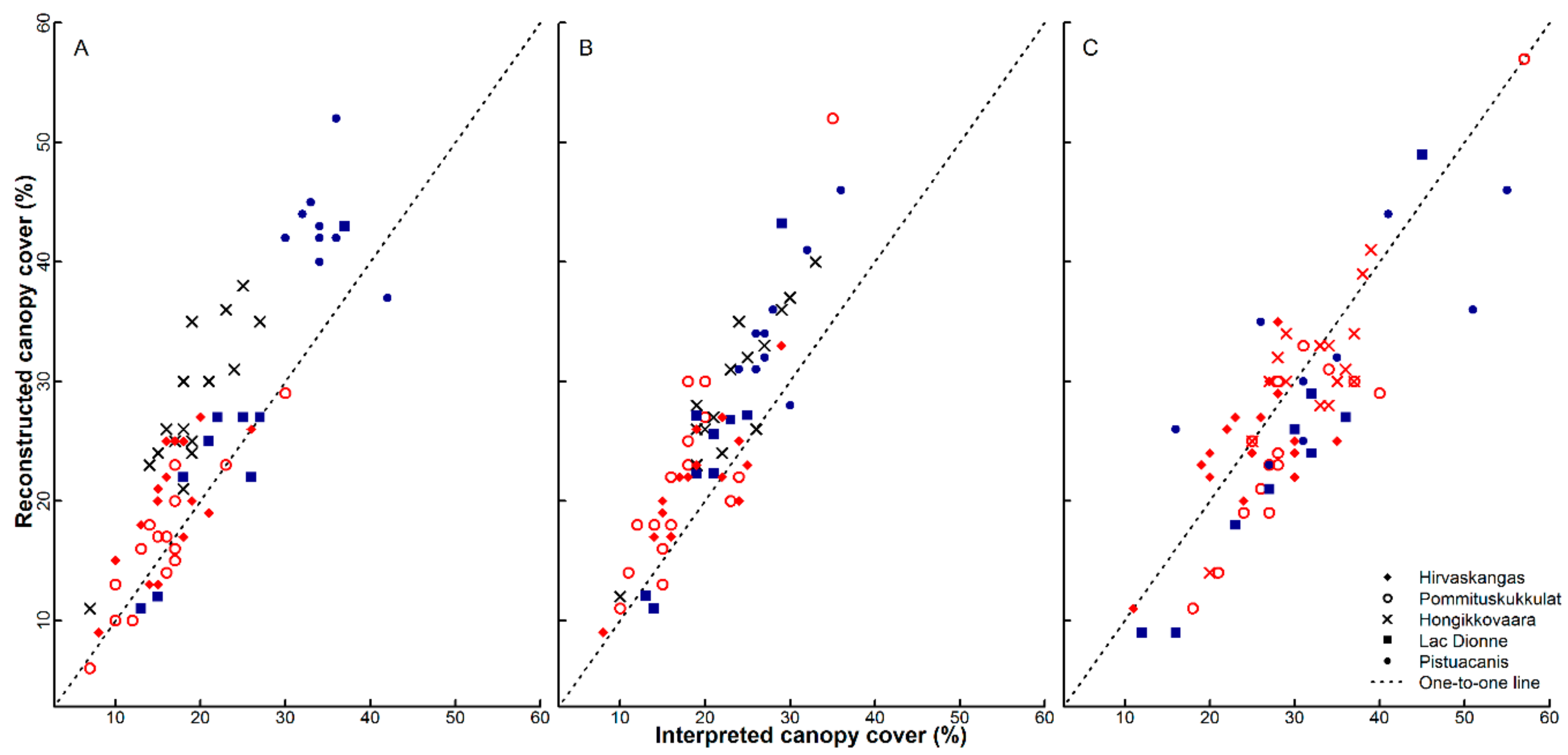
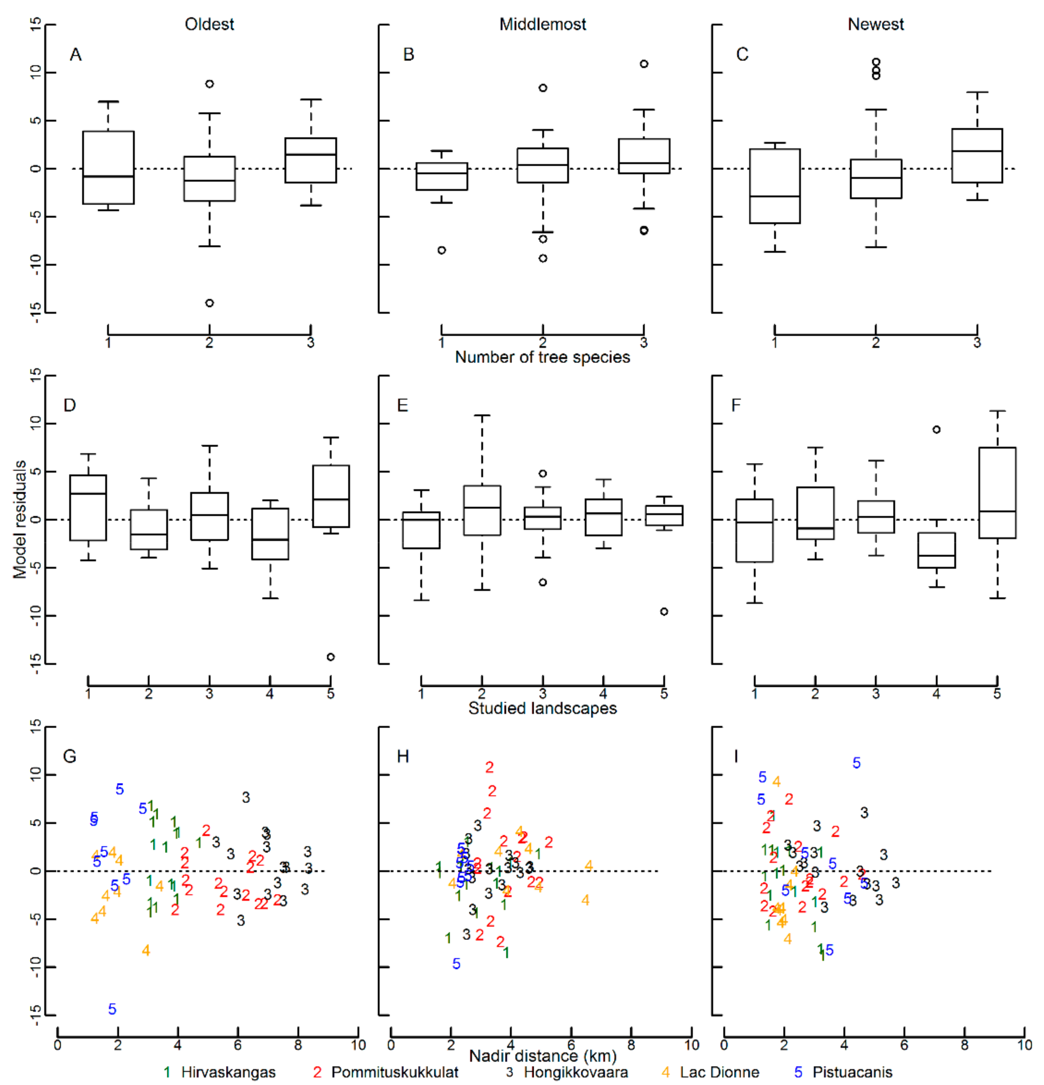
3.1. Bias and Error in the Canopy Cover Interpretation

The difference between the canopy cover reconstructed using the field and tree-ring measurements, and the canopy cover visually interpreted from the aerial photographs ranged from −4 to 15 percentage points (p.p.) (mean ( x ¯ ) = 5 p.p., standard deviation (SD) = ±5 p.p.) in the Finnish landscapes, and from −5 to 16 p.p. ( x ¯ = 5 p.p., SD = ±6 p.p.) in the Quebecois landscapes for the oldest photographs (Figure 1A). The difference varied between −5 and 12 p.p. ( x ¯ = 3, SD = ±4) in the Finnish, and between −4 and 10 p.p. ( x ¯ = 3, SD = ±4) in the Quebecois landscapes for the middlemost photographs (Figure 1B), and between −11 and 7 p.p. ( x ¯ = −2, SD = ±4) in the Finnish, and −15 and 10 p.p. ( x ¯ = −3, SD = ±7) in the Quebecois landscapes for the newest photographs (Figure 1C).
In the calibration models, the coefficient of determination (R2) ranged from 0.61 to 0.79 for the oldest, from 0.68 to 0.89 for the middlemost, and from 0.70 to 0.78 for the newest photographs (Table 2). Similarly, the residual standard error ranges differed between the aerial photographs of varying quality (Table 2).
We illustrate the bias and error differences by comparing the calibrated canopy cover estimates in cells where canopy cover of 20% or 33% was visually interpreted at different times and landscapes. Here, we use models with only the interpreted canopy cover as a predictor (the comparison models for the newest photographs, calibration models for the other photographs). For a cell where 20% canopy cover was interpreted, the 95% prediction intervals for the calibrated canopy cover varied between 15% and 35% for the oldest, between 15% and 32% for the middlemost, and between 7% and 31% for the newest aerial photographs (Figure 2A). For a cell where 33% canopy cover was interpreted, the 95% prediction intervals for the calibrated canopy cover varied between 27% and 52% for the oldest, between 29% and 49% for the middlemost, and between 16% and 43% for the newest aerial photographs (Figure 2B). The mean of the posterior predictive distribution was closest to the interpreted canopy cover in the newest aerial photographs in all landscapes (Figure 2).
The bias in the calibration model residuals was positively related to the number of tree species in the cell (Figure 3A–C). However, the R2 of the model where we explained the calibration model residuals with the number of tree species was only 0.04 (RSE = 3.89). The nadir distance, interpretation order, elevation, slope or the tree species proportions of the total canopy cover in the cell did not cause significant interpretation bias.
To explore the random interpretation error, we analyzed the distribution of the residuals of the model with the least residual bias (the model where we explained the calibration model residuals with the number of tree species). The residual variances varied between the landscapes (Levene’s F = 2.21, p = 0.07; Figure 3D–F), and decreased with increasing the nadir distance (Breusch–Pagan’s BP = 5.66, p = 0.02; Figure 3G–I), but was independent of the photo quality, elevation, slope, interpretation order and the number of tree species.

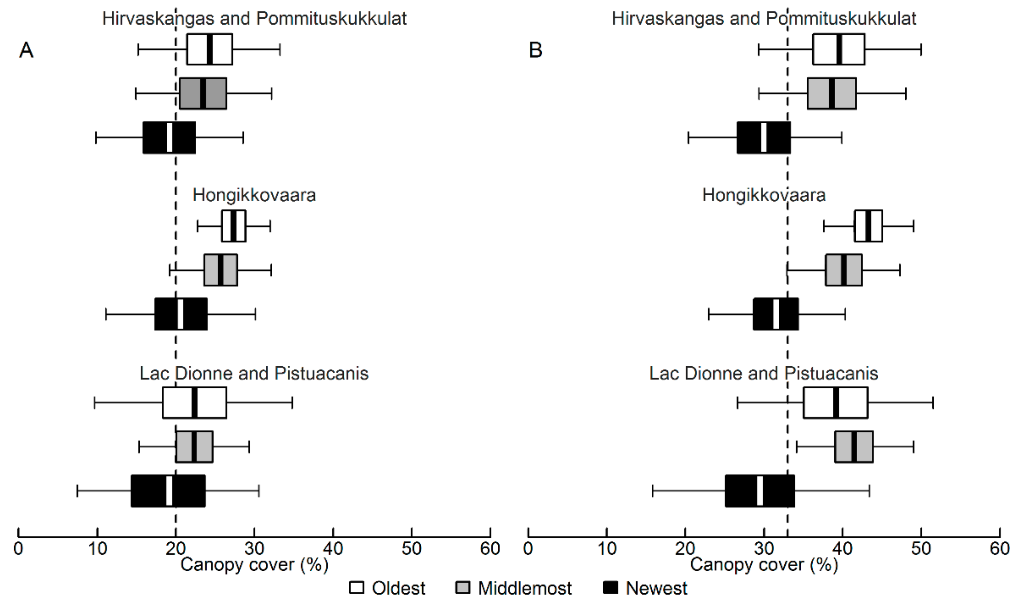
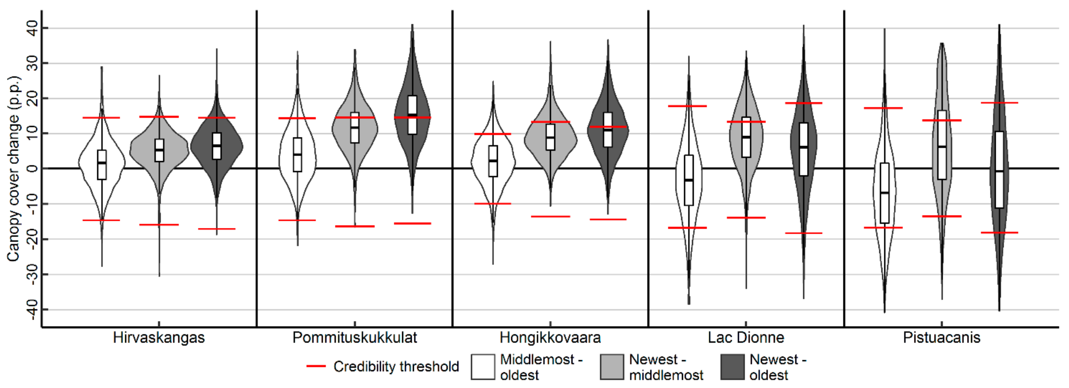
3.2. Canopy Cover Changes and Their Credibilities

Canopy cover in the 0.1-ha cells ranged from 0% to 69%, from 0% to 59%, and from 0% to 70% at the time of the oldest, middlemost and the newest aerial photographs, respectively (Table 3).
The canopy cover changes ranged from −28 to +39 p.p. in the Finnish, and from −42 to +40 p.p. in the Quebecois landscapes at the first study interval (middlemost to oldest in Table 3), and between −31 and +36 p.p. in the Finnish, and between −37 and +36 p.p. in the Quebecois landscapes at the second study interval (newest to middlemost in Table 3). The changes were from −18 to +41 p.p. in the Finnish and from −40 to +41 p.p. in the Quebecois landscapes for the whole study interval (newest to oldest in Table 3). The thresholds between the credible and non-credible positive and negative canopy cover change were located at −15 and +15 p.p. in Hirvaskangas and Pommituskukkulat, −10 and +10 p.p. in Hongikkovaara, and −17 and +18 p.p. in Lac Dionne and Pistuacanis at the first study interval, respectively (Figure 4). The thresholds were −16 and +15 p.p., −14 and +13 p.p., and −14 and +14 p.p. at the second study interval, respectively. The thresholds were −17 and +15 in Hirvaskangas and Pommituskukkulat, −14 and +12 in Hongikkovaara, and −18 and +19 in Lac Dionne and Pistuacanis at the whole study interval. No credible negative canopy cover changes were detected at the study interval between the newest and the oldest photograph in Pommituskukkulat and between the newest and the middlemost and between the newest and the oldest photograph in Hongikkovaara (Figure 4).

4. Discussion

4.1. Bias and Error in the Visual Canopy Cover Interpretation

The visual interpretation bias differed between the aerial photographs of varying quality. Canopy cover was underestimated using the oldest and middlemost, and overestimated using the newest aerial photographs, as indicated by the calibration and comparison models. Varying aerial photo scale and quality cause varying bias in the visual interpretation [9,16]. Our results suggest that the visual interpretation bias depends on the aerial photo scale and quality, most likely because the individual tree crowns appear larger and are easier to delineate from the recent high-quality aerial photographs. This also means that the visual interpretation bias cannot be assumed constant for different quality aerial photographs [23,46], but should be quantified separately for different quality photographs.
The random interpretation error decreased with time (increasing photo quality) only from the middlemost to the newest in Hirvaskangas and Pommituskukkulat, from the oldest to the middlemost in Hongikkovaara, and from the oldest to the middlemost photographs in Quebecois landscapes. Higher photo quality generally facilitates the visual interpretation of aerial photographs [17,18], and improves the interpretation and classification accuracy of forest attributes [12,47]. However, the structural complexity of the interpreted surface [48], variation in tree species composition [21], crown size [13,16] and in the canopy cover [9] may hamper the visual interpretation.
Here, we only measured trees with diameter of ≥10 cm at 1.3-m height in the field. In Quebecois landscapes, the regeneration following the spruce budworm outbreak (from 1970s to mid-1980s) [28] was intense at the time of the newest photographs (2011). Hence, many trees were close to the 10 cm at 1.3-m height limit at the time of the newest photographs. It is likely that the large random error in the interpretation of the newest photographs is caused by the difficulty in separating the trees not measured in the field from those included in the measurements. This difficulty also partially explains the lack of connection between the photo quality and interpretation success.
The interpretation bias varied among the studied landscapes, and depended on the true canopy cover in the interpreted cell. The canopy cover overestimation increased with increasing canopy cover when interpreting the newest photographs. For the oldest and middlemost photographs, canopy cover underestimation increased with increasing canopy cover. Vegetation cover is typically overestimated from aerial photographs, especially if the photo scale is large and vegetation cover exceeds 50% [8]. In the studied landscapes, the canopy cover remained below 60% at all times. Our results suggest that the magnitude of the interpretation bias may depend on the canopy cover, and that the direction of the bias may differ when using aerial photographs with different scale and quality. Moreover, the relationship between the interpretation bias and the canopy cover can also differ between open- and closed-canopy environments [9,23], indicating that similar interpretation bias cannot be assumed if the vegetation cover differs.
The interpretation bias increased with increasing number of tree species, and connected to the proportion of P. abies for the newest photographs in the Finnish landscapes. Increasing number of tree species affects the photo contrast, causes variation in tree crown shapes and sizes, increases the canopy surface roughness and complexity, and thus hampers the visual interpretation [8,21,22]. Moreover, the interpretation success depends on the interpreted tree species and the crown geometry [13]. Hence, the interpretation bias should be quantified separately for landscapes with different tree species compositions.
The random interpretation error varied between landscapes, but was independent of photo quality, elevation, slope, interpretation order and the number of tree species. Especially in the P. mariana-dominated Lac Dionne, the random error differed from the other landscapes. This suggest that the interpretation difficulties could depend on the dominant tree species of the landscape, or on other factors such as different structural complexity (e.g., gap size and abundance, and regeneration) [21,48] or subjective error [20] which causes differences in the interpretation success between the studied landscapes. The varying errors indicate that the errors should be quantified separately for landscapes with different characteristics.
The random interpretation error decreased with increasing nadir distance, especially for the oldest photographs. The trees further away from the nadir appear larger due to different viewing angle [13], and canopy cover should be overestimated when further away from the aerial photo nadir. Hence, the effect of nadir distance to interpretation success should accounted for in the interpretation error estimation.

4.2. Canopy Cover Changes

Magnitude of the credibly detectable canopy cover change differed during different study intervals and among the studied landscapes. The credibility thresholds values which indicate the rate of change needed for credible canopy cover change varied from −18 to −10 p.p. for the negative change and from +10 to +19 p.p. for the positive change. Hence, the canopy cover change which could be credibly detected varied in relation to the study interval and the studied landscape. For example, in Pommituskukkulat, canopy cover decrease of −15 p.p. or increase of +15 p.p. during the first study interval, and decrease of −14 p.p. or increase of +13 p.p. was required for a credible canopy cover change. In most cases, multiple tree crowns are needed to cover an area corresponding to the credibility values, the specific area depending on the absolute canopy cover of a cell. Based on our field data, P. sylvestris or P. abies with the diameter of 200 mm at 1.3-m height had a canopy area of 5.2 m2. The canopy areas were 6.6 m2, 4.2 m2 and 13.3 m2 for A. balsamea, P. mariana and B. pubescens or B. papyrifera with corresponding diameter, respectively. Hence, changes that occur at the level of an individual tree (such as individual tree mortality) could not always be separated from the interpretation error. However, changes occurring at stand scales could already be discerned. Such stand-scale dynamics is common in the forests of both studied regions [2,49].
We discerned credible positive canopy cover changes during all study intervals and at all landscapes. This suggests that the approach can be used to detect the slow and continuous large-scale changes in forest structure, in addition to the abrupt changes commonly studied using aerial photographs and tree-ring analyses [25,26]. Due to the varying temporal scales at which forest structure changes, the ability to analyze both the slow and abrupt changes simultaneously is essential for comprehensive understanding of forest dynamics [50].
We identified less credible negative canopy cover changes during the whole study interval than during the first and the second study intervals in all landscapes. In the Finnish landscapes, credible negative changes occurred during the first and second study intervals, but they were not credibly identified when analyzing the changes during the whole study interval. However, credible negative canopy cover changes were discerned even during the whole study interval (46 years) in Quebec. Tree mortality and regeneration occur constantly at landscape scales, whereas abrupt disturbances induce temporary mortality peaks [3,51]. Our results suggest that the length of the whole study interval (38–52 years, depending on the landscape) is long enough to capture the slow positive changes caused by tree growth and regeneration in both regions, but already too long to capture the negative changes in the Finnish landscapes where severe large-scale disturbances did not occur during the whole study interval. In Quebec, where severe disturbances occurred during the study interval [28], also the whole study interval (46 years) was suitable to discern also the abrupt negative changes. In both regions, the length and timing of observation clearly influenced the observed changes [52].

4.3. Applicability in Other Studies

Here, we were able to discern credible forest structural changes during all study intervals, and in all studied landscapes. Moreover, both slow continuous (positive) changes, and abrupt (negative) changes were detected. Hence, the proposed approach proved feasible for assessing changes in the structure of naturally dynamic boreal forests using repeat aerial photography, while accounting for the error in the historical photographs [14]. The approach can be used to study decadal scale forest biomass changes over vast areas. Besides the boreal biome, the approach can be applied to study forest structural changes in seasonal climate environments (where tree-rings form), using any remotely sensed time series records. For example, Landsat records, and observations from old intelligence satellites (e.g., Corona) have been used in the analysis of temporal vegetation dynamics over decadal scales [6,53]. Moreover, the study extent could be expanded using, for example, automated object-oriented aerial photo analysis [54], or a combination of various remote sensing data [6]. However, for successful bias and error quantification, the size of the field sampling plots should correspond to the size of the interpretation grid cells [55]. Here, the practical limitation related to the calibration data, and the small size of the naturally dynamic forest reserves in Finland limited the study extent.
The error magnitudes differed within and between the studied landscapes. Due to these differences, and because the error might also differ within an aerial photograph due to differences in viewing angle [13,23], tree species composition [21], topography [24] and vegetation cover [9], the calibration data should represent the variability of the studied landscape. The interpretation bias should be carefully assessed to avoid exaggerated change estimation. As manual feature interpretation is subjective [20], our calibration models are not directly applicable elsewhere. However, the proposed approach can be used to calibrate the interpretations, irrespective of the interpreter.
In Quebec, we encountered the temporal limits of our reconstruction procedure for that ecosystem. Here, some of the sites had multiple dead trees (mostly A. balsamea) that had the outer portions of the stems too decayed for cross-dating their year of death. Although we used a bootstrapping procedure that included such trees in the canopy cover reconstruction, this fading-record bias could have caused error in the canopy cover reconstruction if the year of deaths were falsely assigned. This error would then increase uncertainty and influence the magnitude of the credibly detectable canopy cover change. Hence, although the decay rates in the northern boreal forests are generally slow [56], the temporal extent of our approach is limited by tree decay.

5. Conclusions

Visual interpretation bias and error depend on the aerial photo quality and on the attributes of the interpreted landscape. Hence, the same visual interpretation bias and error cannot be assumed for data derived from aerial photographs of varying quality, or for photographs depicting forest landscapes with different tree species compositions. For reliable change quantification, the interpretation bias and error need to be included in the change analysis which bases on the visual interpretation of aerial photographs. Besides the abrupt negative changes, we could also detect the slow forest structural changes that occur continuously over large areas. Due to the wide availability of historical aerial photographs, our approach can be applied for forest change analysis in biomes where tree-rings form.

Author Contributions

Study conception and design, T.A.; Formal analysis, N.K. and L.P.; Investigation, N.K. and T.A.; Methodology, N.K., L.P. and T.A.; Software, T.A.; Validation, L.P. and T.A.; Visualization, N.K.; Writing—original draft, N.K.; and Writing—review and editing, N.K., L.P. and T.A.

Funding

The project was funded by the Academy of Finland (Proj. No. 252629, 276022), Emil Aaltonen Foundation, and the University of Helsinki Funds.

Acknowledgments

We thank Jacques Duval (Quebec Ministry of Natural Resources and Wildlife) for the aerial photographs and digital elevation models for the Quebecois landscapes, and Jussi Lammi and Pasi Myllyniemi (EspaSystems Ltd.), and Ilkka Korpela for support in the stereointerpretation. Antti Ahokas, Nora Arnkil, Stéphane Bourassa, Tapio Kara, Yasuhiro Kubota, Toshihide Hirao, Paavo Ojanen, Maxime Tremblay, and Annukka Valkeapää are thanked for field assistance.

Conflicts of Interest

The authors declare no conflict of interests.

Appendix A

Figure A1. Models between tree diameter and crown projection for: Pinus sylvestris (A); Picea abies (B); Betula pubescens (C); Picea mariana (D); and Abies balsamea (E). For Betula papyrifera, models for Betula pubescens were used. Redrawn from [9].
Forests 09 00631 g0a1
Table A1. Analysis of variance table for testing the pairwise interactions between the interpreted canopy cover, aerial photo quality (oldest, middlemost or newest aerial photograph, proxy for photo quality), and the studied landscape.
PredictorsDegrees of FreedomF-Test ScoreSignificance
Interpreted canopy cover1758.54<0.00
Aerial photo quality241.47<0.00
Studied landscape418.89<0.00
Interpreted canopy cover × Aerial photo quality26.050.00
Interpreted canopy cover × Studied landscape46.98<0.00
Aerial photo quality × Studied landscape84.59<0.00
Model R2 = 0.85, adjusted R2 = 0.83, residual degrees of freedom = 176.
Table A2. Tested calibration models for the newest photographs in the Finnish landscapes. Used predictors were: I_CC = interpreted canopy cover for the cell; P_abies = interpreted proportion of P. abies in the cell; P_sylvestris = interpreted proportion of P. sylvestris in the cell; B_spp = interpreted proportion of birch species in the cell; and AICc = Akaike’s information criteria for small sample sizes.
PredictorsR2RSEAICc
I_CC0.684.41283
I_CC + P_abies0.783.66265
I_CC + P_sylvestris0.743.93275
I_CC + B_spp.0.684.43285
The following notation is used in the Bayesian calibration models:
  • C C i : canopy cover reconstructed from field measurements at plot i in a given landscape or a group of landscapes at a given time point.
  • I _ C C i : corresponding visually interpreted canopy cover
  • n : the sample size.
In vector form: y = [ C C 1 , , C C n ] ) T and I _ C C = [ I _ C C 1 , , I _ C C n ] T . Lets denote by J a n × 1 column vector of ones. The linear regression model is Equation (A1):
y = X β + ϵ
where X = [ J , I _ C C ] , β = [ β 0 , β 1 ] T and ϵ ~ N ( 0 , σ 2 I ) and, I = n × n identity matrix. For the newest time points in Finland also the relative canopy cover of P. abies, R = [ P _ a b i e s 1 , , P _ a b i e s n ] T is included as an explaining variable and hence X = [ J , I _ C C , R ] and β = [ β 0 , β 1 , β 2 ] T . An uninformative prior is used for the unknown parameters β and σ 2 , Equation (A2):
p ( β , σ 2 | X ) σ 2
In this model, the marginal posterior distribution of the regression coefficients is a multivariate t-distribution with ν degrees of freedom, ν = n 2 ( ν = n 3 for the newest Finnish areas; see e.g., [57]), Equation (A3):
β | y , X   ~   t ν ( β ^ , s 2 V β )
where Equations (A4) and (A5):
β ^ = ( X T X ) 1 X T y
V β = ( X T X ) 1
and Equation (A6):
s 2 = 1 ν ( y X β ^ ) T ( y X β ^ )
We model the posterior predictive distributions of the canopy cover for the whole 64 × 64 grid on each time point and area as follows. Let us denote the matrix of explanatory variables in the whole vectorized 64 × 64 grid of a given area by X ˜ , where X ˜ = [ J ˜ , X ˜ , R ˜ ] for the newest Finnish areas and X ˜ = [ J ˜ , X ˜ ] for other areas and times, where J ˜ is a 4096 column vector of ones. The calibrated canopy cover corresponding to X ˜ is then X ˜ β . The calibrated canopy cover is a random variable and has the posterior distribution p ( X ˜ β | y , X , X ˜ ) with mean X ˜ β ^ . However, the variation in such a posterior neglects the variation in the calibrated values caused by the deviations from the regression plane. Therefore, the calibrated canopy cover is modeled as Equation (A7):
y ˜ = X ˜ β + ϵ
where ϵ ~ N ( 0 , σ 2 I ) , where I is the 4096 × 4096 identity matrix. The distribution of y ˜ | y , X , X ˜ is referred to as the posterior predictive distribution and it is (see e.g., [57] for details) Equation (A8):
y ˜ | y , X , X ˜ ~ t ν ( X ˜ β ^ , s 2 ( I + X ˜ V β X ˜ T ) )

References

  1. Kuuluvainen, T.; Hofgaard, A.; Aakala, T.; Jonsson, B.-G. North Fennoscandian mountain forests: History, composition, disturbance dynamics and the unpredictable future. For. Ecol. Manag. 2017, 385, 140–149. [Google Scholar] [CrossRef]
  2. Pham, A.T.; de Grandpré, L.; Gauthier, S.; Bergeron, Y. Gap dynamics and replacement patterns in gaps of the northeastern boreal forest of Quebec. Can. J. For. Res. 2004, 34, 353–364. [Google Scholar] [CrossRef]
  3. Gauthier, S.; Boucher, D.; Morissette, J.; De Grandpré, L. Fifty-seven years of compositional change in the eastern Boreal forest of Canada. J. Veg. Sci. 2010, 21, 772–785. [Google Scholar] [CrossRef]
  4. Hofgaard, A. 50 years of change in Swedish boreal old-growth Picea abies forest. J. Veg. Sci. 1993, 4, 773–782. [Google Scholar] [CrossRef]
  5. Fraver, S.; Jonsson, B.G.; Jönsson, M.; Esseen, P.-A. Demographics and disturbance history of a boreal old-growth Picea abies forest. J. Veg. Sci. 2008, 19, 789–798. [Google Scholar] [CrossRef]
  6. Assal, T.J.; Sibold, J.; Reich, R. Modeling a historical mountain pine beetle outbreak using Landsat MSS and multiple lines of evidence. Remote Sens. Environ. 2014, 155, 275–288. [Google Scholar] [CrossRef]
  7. Fensham, R.J.; Bray, S.G.; Fairfax, R.J. Evaluation of aerial photography for predicting trends in structural attributes of Australian woodland including comparison with ground-based monitoring data. J. Environ. Manag. 2007, 83, 392–401. [Google Scholar] [CrossRef] [PubMed]
  8. Nakashizuka, T.; Katsuki, T.; Tanaka, H. Forest canopy structure analyzed by using aerial photographs. Ecol. Res. 1995, 10, 13–18. [Google Scholar] [CrossRef]
  9. Fensham, R.J.; Fairfax, R.J. Effect of photoscale, interpreter bias and land type on woody crown-cover estimates from aerial photography. Aust. J. Bot. 2007, 55, 457–463. [Google Scholar] [CrossRef]
  10. Kulha, N.; Pasanen, L.; Holmström, L.; De Grandpré, L.; Kuuluvainen, T.; Aakala, T. At what scales and why does forest structure vary in naturally dynamic boreal forests? An analysis of forest landscapes at two continents. Ecosystems 2018. [Google Scholar] [CrossRef]
  11. Jackson, M.M.; Topp, E.; Gergel, S.E.; Martin, K.; Pirotti, F.; Sitzia, T. Expansion of subalpine woody vegetation over 40 years on Vancouver Island, British Columbia, Canada. Can. J. For. Res. 2016, 46, 437–443. [Google Scholar] [CrossRef]
  12. Lydersen, J.M.; Collins, B.M. Change in vegetation patterns over a large forested landscape based on historical and contemporary aerial photography. Ecosystems 2018. [Google Scholar] [CrossRef]
  13. Korpela, I. Individual Tree Measurements by Means of Digital Aerial Photogrammetry. Silva. Fenn. Monogr. 2004. Available online: https://helda.helsinki.fi/bitstream/handle/10138/20665/individu.pdf?sequence=2 (accessed on 15 July 2018).
  14. Lechner, A.M.; Langford, W.T.; Bekessy, S.A.; Jones, S.D. Are landscape ecologists addressing uncertainty in their remote sensing data? Landsc. Ecol. 2012, 27, 1249–1261. [Google Scholar] [CrossRef]
  15. Hughes, M.L.; McDowell, P.F.; Marcus, W.A. Accuracy assessment of georectified aerial photographs: Implications for measuring lateral channel movement in a GIS. Geomorphology 2006, 74, 1–16. [Google Scholar] [CrossRef]
  16. Danby, R.K.; Hik, D.S. Evidence of recent treeline dynamics in southwest Yukon from aerial photographs. Arctic 2007, 60, 411–420. [Google Scholar] [CrossRef]
  17. Fensham, R.J.; Fairfax, R.J.; Holman, J.E.; Whitehead, P.J. Quantitative assessment of vegetation structural attributes from aerial photography. Int. J. Remote Sens. 2002, 23, 2293–2317. [Google Scholar] [CrossRef]
  18. St-Onge, B.; Jumelet, J.; Cobello, M.; Véga, C. Measuring individual tree height using a combination of stereophotogrammetry and lidar. Can. J. For. Res. 2004, 34, 2122–2130. [Google Scholar] [CrossRef]
  19. Hudak, A.T.; Wessman, C.A. Textural Analysis of Historical Aerial Photography to Characterize Woody Plant Encroachment in South African Savanna. Remote Sens. Environ. 1998, 66, 317–330. [Google Scholar] [CrossRef]
  20. Morgan, J.L.; Gergel, S.E. Automated analysis of aerial photographs and potential for historic forest mapping. Can. J. For. Res. 2013, 43, 699–710. [Google Scholar] [CrossRef]
  21. D’Aoust, V.; Kneeshaw, D.; Bergeron, Y. Characterization of canopy openness before and after a spruce budworm outbreak in the southern boreal forest. Can. J. For. Res. 2004, 34, 339–352. [Google Scholar] [CrossRef]
  22. Browning, D.M.; Archer, S.R.; Byrne, A.T. Field validation of 1930s aerial photography: What are we missing? J. Arid Environ. 2009, 73, 844–853. [Google Scholar] [CrossRef]
  23. Massada, A.B.; Carmel, Y.; Tzur, G.E.; Grünzweig, J.M.; Yakir, D. Assessment of temporal changes in aboveground forest tree biomass using aerial photographs and allometric equations. Can. J. For. Res. 2006, 36, 2585–2594. [Google Scholar] [CrossRef]
  24. Teillet, P.M.; Guindon, B.; Goodenough, D.G. On the slope-aspect correction of multispectral scanner data. Can. J. Remote Sens. 1982, 8, 84–106. [Google Scholar] [CrossRef]
  25. Beaty, R.M.; Taylor, A.H. Spatial and temporal variation of fire regimes in a mixed conifer forest landscape, Southern Cascades, California, USA. J. Biogeogr. 2001, 28, 955–966. [Google Scholar] [CrossRef]
  26. Franco, J.A.; Morgan, J.W. Using historical records, aerial photography and dendroecological methods to determine vegetation changes in grassy woodland since European settlement. Aust. J. Bot. 2007, 55, 1–9. [Google Scholar] [CrossRef]
  27. Stephens, S.L.; Skinner, C.N.; Gill, S.J. Dendrochronology-based fire history of jeffery pine-mixed conifer forests in the Sierra San Pedro Matir, Mexico. Can. J. For. Res. 2003, 33, 1090–1101. [Google Scholar] [CrossRef]
  28. Bouchard, M.; Pothier, D. Spatiotemporal variability in tree and stand mortality caused by spruce budworm outbreaks in eastern Quebec. Can. J. For. Res. 2010, 40, 86–94. [Google Scholar] [CrossRef]
  29. Robitaille, A.; Saucier, J.-P. Paysages Régionaux du Québec Méridional; Les Publications du Québec: Sainte-Foy, QC, Canada, 1998; p. 214. [Google Scholar]
  30. Fick, S.E.; Hijmans, R.J. Worldclim 2: New 1-km spatial resolution climate surfaces for global land areas. Int. J. Climatol. 2017, 37, 4302–4315. [Google Scholar] [CrossRef]
  31. Aakala, T. Forest fire histories and tree age structures in Värriö and Maltio Strict Nature Reserves, northern Finland. Boreal Environ. Res. 2018, 23, 209–219. [Google Scholar]
  32. Hennigar, C.R.; MacLean, D.A.; Quiring, D.T.; Kershaw, J.A., Jr. Differences in spruce budworm defoliation among balsam fir and white, red, and black spruce. For. Sci. 2008, 54, 158–166. [Google Scholar] [CrossRef]
  33. Bognounou, F.; De Grandpré, L.; Pureswaran, D.S.; Kneeshaw, D. Temporal variation in plant neighborhood effects on the defoliation of primary and secondary hosts by an insect pest. Ecosphere 2017, 8, E01759. [Google Scholar] [CrossRef]
  34. Bouchard, M.; Pothier, D.; Gauthier, S. Fire return intervals and tree species succession in the North Shore region of eastern Quebec. Can. J. For. Res. 2008, 38, 1621–1633. [Google Scholar] [CrossRef]
  35. Korpela, I. Geometrically accurate time series of archived aerial images and airborne lidar data in a forest environment. Silva. Fenn. 2006, 40, 109–126. [Google Scholar] [CrossRef]
  36. Aakala, T.; Shimatani, K.; Abe, T.; Kubota, Y.; Kuuluvainen, T. Crown asymmetry in high latitude forests: Disentangling the directional effects of tree competition and solar radiation. Oikos 2016, 125, 1035–1043. [Google Scholar] [CrossRef]
  37. Aakala, T. Coarse woody debris in late-successional Picea abies forests in northern Europe: Variability in quantities and models of decay class dynamics. For. Ecol. Manag. 2010, 260, 770–779. [Google Scholar] [CrossRef]
  38. Aakala, T.; Berninger, F.; Starr, M. The roles of competition and climate in tree growth variation in northern boreal old-growth forests. J. Veg. Sci. 2018, in press. [Google Scholar]
  39. Krusic, P.J., Jr.; Hornbeck, J.W. Preserving decayed wood samples for tree-ring measurement. Tree-Ring Bull. 1989, 49, 23–27. [Google Scholar]
  40. Holmes, R.L. Computer-assisted quality control in tree-ring dating and measurement. Tree-Ring Bull. 1983, 43, 51–67. [Google Scholar]
  41. Ilvessalo, Y. Metsänarvioiminen; WSOY: Porvoo, Finland, 1965; p. 400. (In Finnish) [Google Scholar]
  42. Li, R.; Weiskittel, A.R. Estimating and predicting bark thickness for seven conifer species in the Acadian region of North America using a mixed-effects modeling approach: A comparison of model forms and subsampling strategies. Eur. J. For. Res. 2011, 130, 219–233. [Google Scholar] [CrossRef]
  43. Ilvessalo, Y. On the correlation between crown diameter and the stem of the trees. Commun. Ins. For. Fenn. 1950, 38, 1–26. [Google Scholar]
  44. Bivand, R.; Rundel, C. Rgeos: Interface to Geometry Engine—Open Source (Geos), R Package Version 0.3-22; 2016. Available online: https://CRAN.R-project.org/package=rgeos (accessed on 13 March 2018).
  45. Yamaguchi, D.K. A simple method for cross-dating increment cores from living trees. Can. J. For. Res. 1991, 21, 414–416. [Google Scholar] [CrossRef]
  46. Kadmon, R.; Harari-Kremer, R.H. Studying long-term vegetation dynamics using digital processing of historical aerial photographs. Remote Sens. Environ. 1999, 68, 164–176. [Google Scholar] [CrossRef]
  47. Garbarino, M.; Lingua, E.; Subirà, M.M.; Motta, R. The larch wood pasture: Structure and dynamics of a cultural landscape. Eur. J. For. Res. 2011, 130, 491–502. [Google Scholar] [CrossRef]
  48. Zhou, W.Z.; Cadenasso, A.L. Effects of patch characteristics and within patch heterogeneity on the accuracy of urban land cover estimates from visual interpretation. Landsc. Ecol. 2012, 27, 1291–1305. [Google Scholar] [CrossRef] [Green Version]
  49. Caron, M.-N.; Kneeshaw, D.D.; De Grandpré, L.; Kauhanen, H.; Kuuluvainen, T. Canopy gap characteristics and disturbance dynamics in old-growth Picea abies stands in northern Fennoscandia: Is the forest in quasi-equilibrium? Ann. Bot. Fennici 2009, 46, 251–262. [Google Scholar] [CrossRef]
  50. Weed, A.S.; Ayres, M.P.; Hicke, J.A. Consequences of climate change for biotic disturbances in North American forests. Ecol. Monogr. 2013, 83, 441–470. [Google Scholar] [CrossRef]
  51. Aakala, T. Temporal variability of deadwood volume and quality in boreal old-growth forests. Silva. Fenn. 2011, 45, 969–981. [Google Scholar] [CrossRef]
  52. Estes, L.; Elsen, P.R.; Treuer, T.; Ahmed, L.; Caylor, K.; Chang, J.; Choi, J.J.; Ellis, E.C. The spatial and temporal domains of modern ecology. Nat. Ecol. Evol. 2018, 2, 819–826. [Google Scholar] [CrossRef] [PubMed]
  53. Song, D.-X.; Huang, C.; Sexton, J.O.; Channan, S.; Feng, M.; Townshend, J.R. Use of Landsat and Corona data for mapping forest cover change from the mid-1960s to 2000s: Case studies from the Eastern United States and Central Brazil. ISPRS J. Photogramm. Remote Sens. 2015, 103, 81–92. [Google Scholar] [CrossRef]
  54. Laliberte, A.S.; Rango, A.; Havstad, K.M.; Paris, J.F.; Beck, R.F.; McNeely, R.; Gonzalez, A.L. Object-oriented image analysis for mapping shrub encroachment from 1937 to 2003 in southern New Mexico. Remote Sens. Environ. 2004, 93, 198–210. [Google Scholar] [CrossRef]
  55. Næsset, E. Predicting forest stand characteristics with airborne scanning laser using a practical two-stage procedure and field data. Remote Sens. Environ. 2002, 80, 88–99. [Google Scholar] [CrossRef]
  56. Aakala, T.; Kuuluvainen, T.; Wallenius, T.; Kauhanen, H. Contrasting patterns of tree mortality in late-successional Picea abies stands in two areas in northern Fennoscandia. J. Veg. Sci. 2009, 20, 1016–1026. [Google Scholar] [CrossRef]
  57. Gelman, A.; Carlin, J.B.; Stern, H.S.; Rubin, D.B. Bayesian Data Analysis, 2nd ed.; Chapman & Hall/CRC: London, UK, 2004; p. 668. [Google Scholar]
Figure 1. Comparison between the canopy cover reconstructed using the field and tree-ring measurements, and the visually interpreted canopy cover at the time of the: oldest aerial photographs (A); middlemost aerial photographs (B); and newest aerial photographs (C). The symbols indicate the landscapes, and the symbol colors indicate the landscapes which were calibrated using the same calibration model.
Forests 09 00631 g001
Figure 2. The canopy cover posterior predictive distributions for a cell for which canopy cover of 20% (A) or 33% (B) was interpreted at the time of the oldest (white), middlemost (grey) and newest (black) aerial photographs. The distributions are produced with models where only the interpreted canopy cover was used as a predictor (the comparison models for the newest photographs, calibration models for the other photographs). The whiskers indicate the 95% prediction intervals.
Forests 09 00631 g002
Figure 3. Calibration model residuals in relation to the number of tree species in the field-sampled cells (AC), and the residuals from the model with least residual bias (the model where we explained the calibration model residuals with the number of tree species) in the studied landscapes (DF) and in relation to the nadir distance (GI) for the oldest (first column), middlemost (second column) and the newest (third column) aerial photographs.
Forests 09 00631 g003
Figure 4. The canopy cover change distributions for the 0.1-ha cells for the first study interval (white), for the second study interval (light grey) and for the whole study interval (dark grey) in each landscape as percentage points (p.p.). The violins indicate the distribution of the change values in the given landscape and the study interval. The boxplots within the violins indicate the interquartile range of the data. The bottom boxplot whisker indicates the Q1 − 1.5 × interquartile range, and the topmost whisker the Q3 + 1.5 × interquartile range. The red lines are the credibility thresholds. The cells above the topmost threshold have credible positive canopy cover change, and the cells below the bottom threshold have credible negative change.
Forests 09 00631 g004
Table 1. The photographs used in the study. The Finnish aerial photographs are from the National Land Survey Finland, except for the 1972 photo in Hongikkovaara and 1991 photo in Hirvaskangas which are from the Finnish Defence Forces, and the middlemost photos in Pommituskukkulat and Hongikkovaara which are from Blom Geomatics AS. The newest Quebecois photographs are from Ministère des Forêts, de la Faune et des Parcs du Québec, and the older photographs from Geomatheque Ltd., QC, Canada.
Oldest PhotographsMiddlemost PhotographsNewest Photographs
YearScalePixel Size (m)YearScalePixel Size (m)YearScalePixel Size (m)
Hirvaskangas19591:30,0000.619911:31,0000.420111:20,0000.5
Pommituskukkulat19591:30,0000.919881:30,0000.420111:20,0000.5
Hongikkovaara19721:60,0000.919881:30,0000.420101:20,0000.5
Lac Dionne19651:16,0000.219871:15,0000.220111:11,0000.3
Pistuacanis19651:16,0000.219871:15,0000.220111:11,0000.3
Table 2. The calibration model parameters for the oldest, middlemost and newest aerial photographs. R2-column shows the model coefficient of determination, α the intercept, b the slope, and (RSE) the residual standard error. In the calibration model for the newest photographs in the Finnish landscapes, b1 is the interpreted canopy cover and b2 is the proportion of P. abies of the interpreted canopy cover.
Hirvaskangas and PommituskukkulatHongikkovaaraLac Dionne and Pistuacanis
R2αbRSER2αbRSER2αbRSE
Oldest0.613.140.933.510.754.191.243.410.79−3.841.315.70
Middlemost0.680.921.154.340.832.871.132.760.89−7.281.493.13
Newest0.785.20b1 0.84
b2 −7.59
3.660.785.20b1 0.84
b2 −7.59
3.660.702.740.816.14
Table 3. The mean canopy cover, canopy cover standard deviations and canopy cover ranges calculated from the oldest, middlemost and the newest aerial photographs, and the mean canopy cover change (as p.p.), its standard deviation and range for the studied time intervals.
HirvaskangasPommitus-kukkulatHongikkovaaraLac DionnePistuacanis
MeanSDRangeMeanSDRangeMeanSDRangeMeanSDRangeMeanSDRange
Oldest photograph1840–351640–292060–432150–6937100–62
Middlemost photograph2040–432050–402250–412170–513090–59
Newest photograph2660–593380–633260–6026130–5437120–70
Middlemost–oldest17−28–3948−22–3427−27–25−311−39–32−713−42–40
Newest–middlemost55−31–27127−17–3496−11–3698−34–33713−37–36
Newest–oldest76−18–34169−13–41117−13–37612−37–41015−40–41

