Assessment of Red-Edge Position Extraction Techniques: A Case Study for Norway Spruce Forests Using HyMap and Simulated Sentinel-2 Data

Abstract

Systematic quantification and monitoring of forest biophysical and biochemical variables is required to assess the response of ecosystems to climate change and gain a deeper understanding of the carbon cycle. Red-Edge Position (REP) is a hyperspectrally detectable parameter, which is sensitive to Chlorophyll (Chl) content. In the current study, REP was modelled for Norway spruce Forest canopy Reflectance and Transmittance (FRT) using Radiative Transfer Modelling (RTM) (resampled to HyMap and Sentinel-2 spectral resolution) as well as calculated from the real HyMap and simulated Sentinel-2 image data. Different REP extraction methods (PF, LE, 4PLI and its optimized versions for HyMap and Sentinel-2 spectral resolution) were assessed. The lowest differences in REP values calculated from image-extracted spectra and from the theoretical RTM simulations were found for the 4PLI method including its HyMap and Sentinel-2 optimized versions (4PLIH and 4PLIS). Despite its simplicity, the 4PLI REP extraction technique demonstrated its potential usefulness for estimating canopy chlorophyll (Chl × LAI) content using both airborne hyperspectral (HyMap) data as well as space-borne Sentinel-2 image data.

1. Introduction

Leaf pigments have been identified as important indicators of physiological status, senescence and stress [1,2,3], while Chlorophyll (Chl) is the leaf pigment responsible for photosynthesis. Estimates of foliar biochemicals such as the level of Chl provide us with information on the plant’s development stage, productivity and stress [2,4,5]; therefore, Chl is one of the key biophysical variables used for vegetation monitoring. Direct field methods using standard approaches for estimating Chl content frequently require destructive harvesting and they are labour-intensive and costly.

The biochemical characteristics of vegetation, including Chl, affect its spectral properties and remote sensing, especially hyperpspectral remote sensing, offers an alternative set of techniques in different domains, such as laboratory measurements, field and imaging spectroscopy; therefore, it has opened new ways of monitoring Chl content over a wide range of scales [6,7].

The relationship between the spectral properties of vegetation and the biochemical and biophysical properties can be studied using empirical correlations. Such approaches are relatively straightforward but unfortunately lack robustness as the empirical correlations of vegetation’s spectral properties and biophysical/biochemical parameters are site and time specific. To overcome this, physical models have been developed. Physical methods employ inverted Radiative Transfer (RT) models (e.g., PROSPECT [8,9], LEAFMOD [10], SAIL [11] and SCOPE [12]) to estimate the biochemical content at the leaf level [13]. RT modeling simulates the transfer of radiation in the canopy by computing the interaction between a plant and solar radiation [14,15]. In comparison with the direct extrapolation and the canopy-integrated approaches, inversion models offer the potential of a more generic approach to quantify the biochemical parameters of vegetation based on spectral data. However, numerous in-put parameters are requested for the RT models, which are still difficult and costly to obtain for regional studies.

The wavelength of the maximum slope in the region of the red-edge (680 to 780 nm), termed the Red-Edge Position (REP) [16,17], is a spectral measure that is less sensitive to the effect of variable leaf and canopy Chl content and environmental conditions on Chl content estimation. REP is an important index that indicates the abrupt leaf reflectance change between 680 nm and 780 nm of the vegetation spectra caused by the combined effects of strong Chl absorption and leaf internal scattering [18]. Increases in the amount of Chl result in a broadening of the major Chl absorption feature centred around 680 nm [18,19], causing a shift in the slope and REP towards longer wavelengths [16,20,21,22]. Therefore, REP, due to it being sensitive to Chl variation, provides a valuable remote sensing means for estimating leaf or canopy Chl content [20,23,24]. Various techniques have been developed for the extraction of REP parameters from different sources of spectral data, among the most widely used REP extraction methods are such methods as the Maximum First Derivative (MFD) [22,25,26,27,28], the Polynomial Fitting (PF) technique [29], the Inverted Gaussian (IG) technique [30] and Linear Extrapolation (LE) technique [7].

While laboratory, field and imaging spectroscopy have been used to extract REP and estimate Chl content, new opportunities are approaching since the new state-of-the-art satellite, Sentinel-2A, was launched on 23 June 2015. Sentinel-2A (S2), a superspectral instrument, is the first satellite of the S2 constellation carrying 13 bands, covering the Visible-Near Infrared (VNIR) and Shortwave-Infrared (SWIR) domains with a spatial resolution ranging from 10 to 60 m. Effective utilization of S2 data, which is now in orbit, provides a very good opportunity for vegetation studies on a regional and continental level especially due to the high revisit time of S2 satellites [31,32,33,34]. In addition, S2 data contain more spectral bands within the red-edge than data provided by e.g., Landsat, ASTER and other multispectral space-borne instruments. This allows such techniques as REP calculation, which were originally developed for hyperspectral data, to be employed for S2 data. This is specially related to the bands centred at 665 (band 4), 705 (band 5), 740 (band 6) and 783 (band 7) nm [35].

The potential of S2 data has been investigated for diverse vegetation parameter estimations such as LAI [36,37,38], Chl and nitrogen [39], biophysical parameters [31,40] and REP [39,41]. However, only a limited number of forest-oriented applications have been published so far. This may be due to the fact that forests are generally more challenging targets than agricultural fields, as it is also much more time and cost-demanding to collect the ground-truth data. In addition, the architectural structure, clumping of optically active surfaces at multiple scales and spatial-temporal foliage dynamics contribute to this problem. Assessment of forest biophysical and biochemical variables faces further complexity by the contribution of vegetation, litter, soil, bark as well as plant and relief shadow, all of which influence the radiometric signal [42]. As a result, all these factors together make forest-oriented remote sensing applications more challenging than compared to agriculture ones. Only three studies have been published so far on this topic: one deals with discrimination of tropical forests types using hyperspectral and simulated S2 data [33]. In the second one, the potential of EnMap and S2 data was assessed for detecting drought stress phenomena in deciduous forests [32]. The third study, which is the only one so far that utilizes the real S2 data rather than simulated datasets, deals with the suitability of the S2 red-edge wavelengths for burn severity discrimination [43].

The main goal of this paper was to test REP extraction methods while focusing on those suitable for both the broader-band hyperspectral data used in this study (e.g., HyMap) as well as for space-borne S2 data. This study was forest-oriented and intends to answer the following questions: (i) What are the differences in the REP values calculated from the theoretical Radiative Transfer Model (RTM) simulations and the real (hyperspectral-image-extracted) spectra, and which of the studied REP calculation methods provides the best fit between the theoretical RTM simulations and the real hyperspectral image data (HyMap)? (ii) What is the influence of spectral sampling on the REP calculation reliability (comparison of theoretical RTM simulations, real hyperspectral image data (HyMap) and simulated S2 data)? (iii) What do the relationships between the calculated REP values and canopy Chl (Chl × LAI) content look like when using the theoretical RTM simulations, real hyperspectral image data (HyMap) and simulated S2 data?

2. Materials and Methods

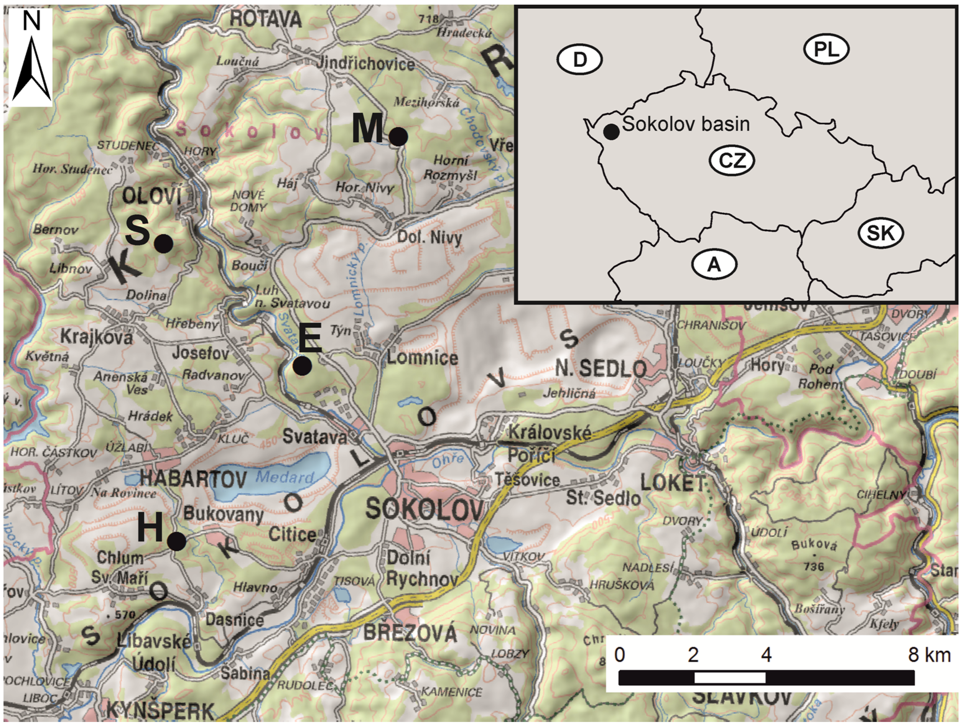
2.1. Study Area

The study was performed in the Sokolov lignite basin situated in the western part of the Czech Republic. This region has been affected by long-term lignite mining and heavy industrial pollution. The central part of the basin is surrounded by boreal forests with Norway spruce (Picea abies L. Karst.) as the predominant species, which is the main object of interest in this study. The current research was conducted for four homogeneous (i.e., single-species and evenly aged) Norway spruce forests stands: Erika (E), Habartov (H), Mezihorská (M) and Studenec (S) located in the neighbourhood of the lignite mining area. The trees did not show any visible symptoms of damage at the time of data acquisition [44], although these forests are situated in an area with a historically high level of environmental pollution. The location of the Sokolov lignite basin with the positions of the studied Norway spruce stands can be seen in Figure 1.

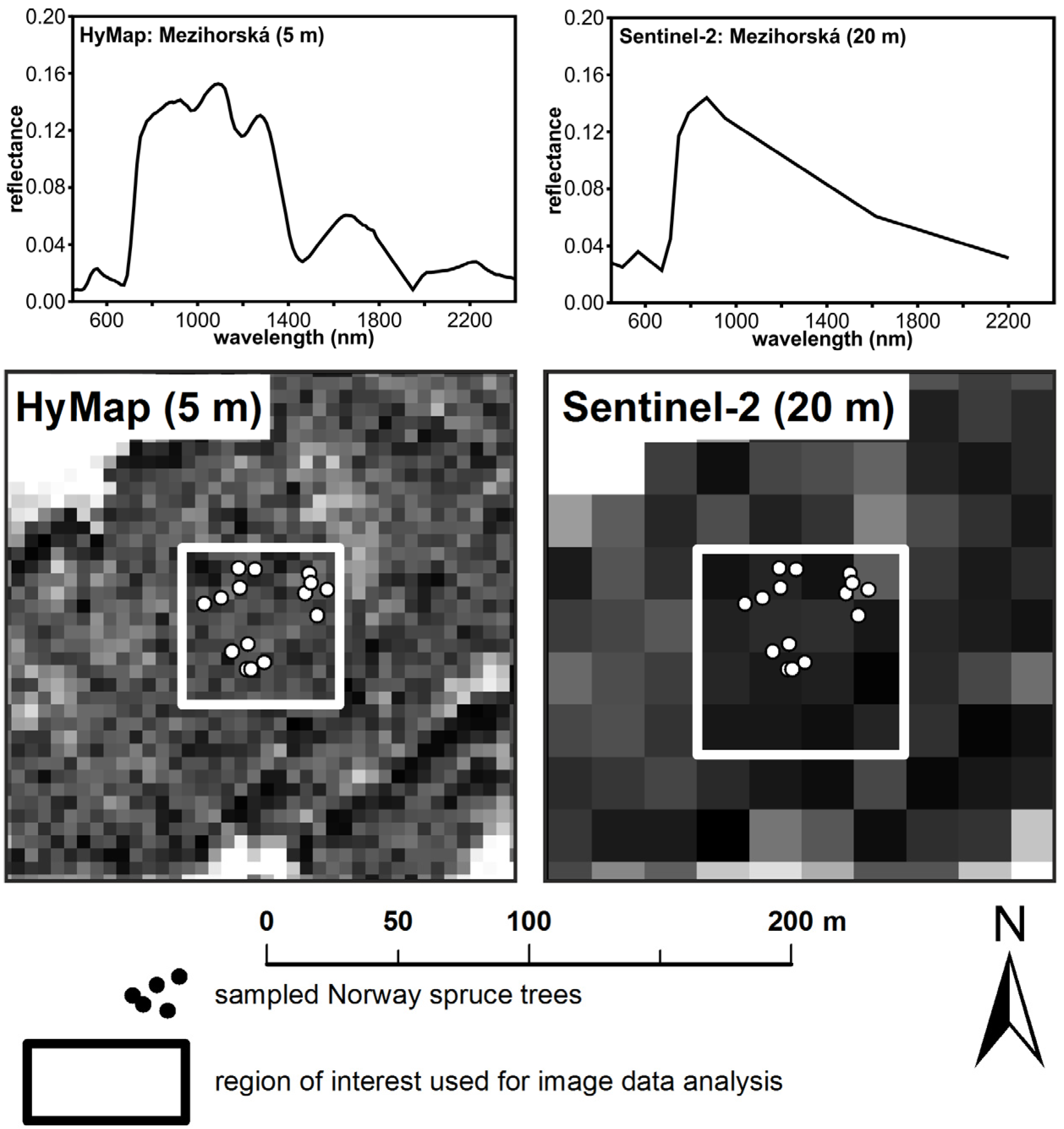
2.2. Airborne Hyperspectral Data Acquisition

Two HyMap airborne hyperspectral datasets were acquired over the area of interest. On 27 July 2009, the instrument was flown at an average altitude of 2570 m and nine cloud-free flight lines in a NE-SW direction were obtained with a ground spatial resolution of 5 m. The second HyMap dataset was acquired on 21 August 2010, obtaining seven cloud-free flight lines at an average altitude of 2475 m with 4 m ground spatial resolution. Both datasets covered the spectral range between ca. 450–2500 nm with a FWHM of ca. 10–15 nm.

The atmospheric correction was performed using the ATCOR-4 software with the aerosol optical thickness obtained from in-situ measurements by a Microtops II Sunphotometer. For validation purposes, the Hemispherical-Conical Reflectance Factors (HCRF) of several near-Lambertian surfaces (asphalt, concrete, artificial grass and a water pool) were measured. The data were acquired using an ASD FieldSpec 3 spectroradiometer, equipped with a standard pistol grip, simultaneously with the airborne data acquisition. Since the HyMap data showed strong Bidirectional Reflectance Distribution Function (BRDF) effects due to the wide field of view, semi-empirical nadir normalization was performed using the Ross-Li kernel approach [45,46]. Ortho-georectification of the 2009 dataset was performed in PARGE software, while the 2010 data were corrected using the ORTHO module. More details about the HyMap 2009 and 2010 data pre-processing can be found in Kopačková et al. [44].

2.3. Simulated Sentinel-2 Image Data

Sentinel-2 data was simulated using the S2 end-to-end simulation tool (S2eteS), which is described in detail in Segl et al. [47]. It consists of a forward simulation module and a backward simulation module.

The forward simulation consists of a spatial module, a spectral module, an atmospheric module and a spectral module. The spatial module creates a virtual S2 sensor overpass over the image scene, taking into account parameters such as the specific sensor observation geometry Segl et al. [47]. The atmospheric module converts the surface reflectance data to Top Of Atmosphere (TOA) reflectance taking into account atmospheric parameters such as e.g., Aerosol Optical Thickness (AOT), variable Columnar Water Vapour (CWV), followed by a radiance calculation. The spectral module performs the spectral resampling of the resulting data. The resultant at-sensor radiance is converted to DN in the radiometric module considering e.g., sensor noise and detector nonlinearity Segl et al. [47].

The backward simulation then uses the S2 pre-processing chain to retrieve simulated-at-ground reflectance data, which include the aforementioned sensor specific parameters. More detailed information on the whole simulation process can be found in Segl et al. [47].

This allows a close-to-real sensor simulation of the S2 data, rather than just a simple spectral and spatial resampling of the HyMAP data to S2 data. Therefore, this approach allows close-to-real-world tests and demonstrations of S2 applications such as, for example, mapping of iron-bearing surface cover types [48] or the REP calculation prior to the launch of the sensor presented here.

2.4. In-Situ and Laboratory Measurement of Vegetation Properties

The needle sampling scheme was described in detail in Kopačková et al. [44]. In this study, the Chl content determined for the Upper (U₁) portion of the sunlit crown of 50 mature Norway spruce trees at four study sites was used: Erika (10 trees), Habartov (15 trees), Mezihorská (15 trees) and Studenec (10 trees). The samples were collected from the same trees in both years. The total Chl was extracted in DiMethylForamide (DMF) based on Porra et al. [49]. The foliar pigment content was then calculated using the equations of Wellburn [50]. The samples were scanned by a table scanner to determine their projection area (LAP), which was then transformed to the total needle area (LAT) using the LAP/LAT empirical correction factors [51]. LAT was then used to calculate the Specific Leaf Area (SLA) describing the ratio of needle total area and dry weight. The SLA values were finally used to normalize the values of Chl by sample area. Another part of the collected samples was used for the spectral measurement of the needles using ASD FieldSpec 3 [52]. In addition, the spectra of Norway spruce bark and dry litter were measured as inputs for the canopy RTM. These measurements were performed using the SR-2500 spectroradiometer (Spectral Evolution Inc., Lawrence, MA, USA) combined with the contact probe.

A set of Digital Hemispherical Photographs (DHP) was acquired at each site in order to estimate the canopy biophysical and structural parameters using a Canon EOS 400D camera (Canon Inc., Tokyo, Japan) equipped with a Sigma 4.5 mm Circular fisheye lens. The acquired DHPs were pre-processed in GIMP 2.8 software (GIMP Development Team). CanEye software (Canon Inc., Tokyo, Japan) was finally used to estimate the true and effective Leaf Area Index (LAI), CAnopy Closure (CAC) and CRown Cover (CRC).

2.5. Leaf and Canopy Radiative Transfer Modelling

The ASD reflectance acquired for the needle sample calibration dataset (2 × 30 samples) was used for the parameterization of the PROSPECT-5 leaf RTM [8,53]. This model was introduced by Jacquemoud and Baret [8] and currently it is one of the most frequently used leaf-level RTM due to its simplicity and very good inversion ability [9], which were the main reasons for using this model. A validation dataset (2 × 20 samples) was used for an independent assessment of the needle simulations. The main outputs of PROSPECT-5 forward simulations are single-leaf Reflectance (R) and Transmittance (T) at particular wavelengths. PROSPECT-5 was run in the forward mode with known values of Chl on the input with a structural parameter N ranging from 1.0 to 5.0 (0.1 step). The simulated R and T were transformed to infinite reflectance (R_∞) using the equations of Zarco-Tejada and Miller [54] as the ASD outputs (when using a contact probe to measure needle reflectance) have more the character of R_∞:

$$R_{\infty }=\frac{R}{1-T^2}$$

(1)

where: R_∞ is infinite reflectance at the wavelengths lambda; R is single leaf reflectance at wavelength lambda; T is single leaf transmittance at wavelength lambda.

Infinite reflectance (R_∞) is defined as the reflectance of a leaf stack where the influence of multiple radiation scattering is taken into account. The simulated R_∞ spectra were then compared with the ASD reflectance to find the optimal value of the parameter N using the Root Mean Square Error (RMSE) merit function minimization technique. The optimal N value was used together with the Chl values of the validation dataset samples to assess the accuracy of the PROSPECT-5 simulations. The simulated spectra were again transformed from R and T to R_∞ and then compared with the corresponding measured ASD spectra of the validation dataset used for calculating the RMSE of simulation.

The simulated R and T were up-scaled to the shoot level using the spectral invariants theory following Rautiainen et al. [55]. This theory is based on an assumption that the canopy albedo at the given wavelength λ is related to leaf/needle albedo on the same wavelength λ trough, the photon recollission probability p [56,57]) and represents an alternative approach for modelling the radiation scattering occurring in a vegetation canopy. U₁ shoot-level spectra were simply averaged to obtain the single-shoot-level spectrum for each sampled tree. Mean shoot-level spectra were then determined for each particular stand by averaging the spectra of the corresponding sampled trees, which were finally used as the input of the canopy RTM.

The FRT model was used for up-scaling the needle/shoot-level spectra to the canopy [58]. One single mock-up (a file definition of the properties of the vegetation stand whose spectral signature is going to be simulated by the model) was prepared for all the studied sites. First, Diameter Breast Height (DBH) and crown radius (R_c) were determined using a combination of in-situ and two allometric equations [59] as below:

$$h=1.3+\frac{{\mathrm{DBH}}^2}{6.22+0.131\mathrm{DBH}+0.0317{\mathrm{DBH}}^2}$$

(2)

$$R_{\mathrm{c}}=0.5\left(0.2195+0.2545\ln \left(\mathrm{DBH}\right)+0.009h-0.6735\ln \left(\frac{h}{\mathrm{DBH}}\right)\right)$$

(3)

where: h is tree height; DBH is diameter breast height; R_c is crown radius.

Crown Cover (CRC) was calculated from estimated CAC by processing the DHPs and the given fixed value of the tree distribution parameter (TDP = 1.5) [59]. Then, the tree density was estimated using the CRC and R_c values. The Dry Leaf Weight (DLW) was finally calculated from the Density (DEN) (determined in the previous step), Specific Leaf Weight (SLW) and LAI (estimated from the DHPs). The measured Norway spruce bark spectrum was used to define the spectral properties of the wooden parts of the trees considered in the FRT model and the measured dry litter spectrum was utilized as the forest floor understory background spectrum. The parameterized FRT model was run in the forward mode to provide a canopy spectrum for each considered forest stand. The simulated spectra were resampled from the original 5 nm sampling to the spectral resolution of the HyMap and S2 data. Finally, they were compared with the corresponding spectra extracted from the HyMap and simulated S2 image data.

2.6. Red-Edge Position Calculation

The REP, resampled to HyMap and S2 spectral resolution, was calculated from the FRT canopy RTM as well as from the real HyMap (5-m spatial resolution) and simulated S2 imagery (20-m spatial resolution). The REP values extracted from the FRT simulations are signed as REP_SIM and the values calculated from the image datasets are signed as REP_IMG in the following text. Each Norway spruce stand was determined by Regions Of Interest (ROI) (Figure 2). The spatial extend of the ROI was defined with respect to the S2 data spatial resolution (20 m) In order to obtain representative statistical inputs in terms of HyMap/S2 spatial resolutions and the spatial distributions of sampling points used for the Chl × LAI content estimation, the image pixels were grouped to ROIs. The same ROI was used in both HyMap (5-m spatial resolution) and simulated S2 imagery (20-m spatial resolution). The spectra of the pixels falling within the ROI were used in the following analyses (e.g., REP assessment). The averaged REP values derived for each ROI were then correlated with the per-ROI-averaged Chl × LAI content (see more in Section 2.8).

To derive the REP from the HyMap, the polynomial fitting (PF) method and Linear Extrapolation (LE) were employed as well as the 4-Point Linear Interpolation (4PLI) in its general form (4PLI) and in the form tuned for the spectral resolution of HyMap (4PLIH) [31]. To derive the REP from the S2, the 4-Point Linear Interpolation method adjusted to the spectral resolution of S2 data was employed (4PLIS). Each algorithm is designated based on the following formulae:

2.6.1. Polynomial Fitting (PF)

A polynomial function was least-squares-fitted to the reflectance spectrum between the wavelengths, corresponding to the minimum reflectance in the red and the maximum NIR (shoulder) reflectance:

$$R_{\mathsf{\lambda }}=a_0+{\displaystyle \sum _{i=1}^a{a}_i{\mathsf{\lambda }}^i}$$

(4)

where: λ is the band between 670 nm to 780 nm.

The REP is determined using the first derivative of the function used for approximating the source spectrum.

The advantage of this method is that it is only necessary to set the spectral range.

2.6.2. Linear Extrapolation (LE)

This method is based on the supposition of the REP location at the intersection of the Far Red Line (FRL) and Near Infrared Line (NIL) defined by the first derivative of the reflectance at 680 and 700 nm (FRL) or 725 and 760 nm (NIL). For the HyMap spectral resolution can be defined as:

$$\mathrm{FRL}=a_1\mathsf{\lambda }+b_1$$

(5)

$$a_1=\frac{D_{676}-D_{705}}{676-705};b_1=D_{705}-\frac{705\cdot \left(D_{676}-D_{705}\right)}{676-705}$$

(6)

NIL is defined as:

$$\mathrm{NIL}=a_2\mathsf{\lambda }+b_2$$

(7)

$$a_2=\frac{D_{719}-D_{762}}{719-762};b_2=D_{760}-\frac{762\cdot \left(D_{719}-D_{762}\right)}{719-762}$$

(8)

where: a₁ and a₂ are the gains of FRL resp. NIL; b₁ and b₂ are offsets of FRL resp. NIL; D₆₈₀, D₇₀₀, D₇₂₅ and D₇₆₀ are first derivatives of the reflectance at 680, 700, 725 and 760 nm, respectively.

REP is then defined as:

$$\mathrm{REP}=\frac{-\left(b_1-b_2\right)}{\left(a_1-a_2\right)}$$

(9)

2.6.3. 4-Point Linear Interpolation (4PLI)

It is assumed that the reflectance curve at the red-edge can be approximated by a straight line centred near the mid-point between the reflectance at 780 nm and 670 nm. As such, it is, in a general form, defined as:

$$\mathrm{REP}=700+40\cdot \left(\frac{\left(\frac{R_{670}+R_{780}}{2}\right)-R_{700}}{R_{740}-R_{700}}\right)$$

(10)

The form adjusted to the HyMap data resolution is defined as:

$$\mathrm{REP}=705+43\cdot \left(\frac{\left(\frac{R_{676}+R_{776}}{2}\right)-R_{705}}{R_{748}-R_{705}}\right) [\text{4PLIH}]$$

(11)

The form adjusted to the S2 data resolution is defined as:

$$\mathrm{REP}=705+35\cdot \left(\frac{\left(\frac{R_{783}+R_{665}}{2}\right)-R_{705}}{R_{740}-R_{705}}\right) [\text{4PLIH}]$$

(12)

where: R₆₇₀, R₇₈₀, R₇₀₀ and R₇₄₀ are the reflectance values at 670, 780, 700 and 740 nm, respectively.

2.7. Comparison between REP_IMG and REP_SIM

REP_SIM and REP_IMG were then compared for each individual REP extraction method (4PLI, PF, LE, 4PLIH and 4PLIS). The fits of the REP_SIM and REP_IMG values were expressed in terms of RMSE and coefficient of determination (R²). The RMSE was calculated based on the following equation:

$$\mathrm{RMSE}=\frac{{{\displaystyle \sum \left({\mathrm{REP}}_{\mathrm{IMGi}}-{\mathrm{REP}}_{\mathrm{SIMi}}\right)}}^2}{n}$$

(13)

where: REP_IMGi is the REP value extracted from the image data for the forest stand i; REP_SIMi is the REP value extracted from the FRT simulated spectra for the forest stand i; n is the number of forest stands (in this case n = 4).

The calculated REP_SIM and REP_IMG for HyMap and S2 spectral resolution were compared with the REP values considered as the comparative standard (REP_STD). This comparative standard was defined as the REP value extracted from the original FRT simulations using the PF method because: (i) the spectral resolution of the original FRT simulations (5 nm) is higher than the spectral resolution of the HyMap data and much higher than the spectral resolution of the S2 data; (ii) the reflectance curves can be approximated by a polynomial function with very high accuracy; (iii) the PF is the only fully continuous REP extraction method in contrast to other methods based on discrete approaches using various types of inter or extrapolations.

Comparing the REP_SIM values extracted from the HyMap and S2 level spectra with the standard REP_STD, we can observe the influence of the spectral resolution on the REP calculation accuracy: the REP_SIM values are calculated from the simulated spectra that differs from the spectra used for calculating the standard value only by the spectral resolution. Comparing the REP_IMG values with the standard enables a study of precisely how it is possible to find the real REP value using the real imagery and which REP extraction method is optimal in each case.

2.8. Vegetation Properties and REP Correlation

As described in Section 2.6, the REP values derived for each ROI were then correlated with the per-ROI-averaged Chl × LAI content (Figure 2). In this specific case, for each of 4 sites one representative Chl × LAI value was obtained, an average value of 10 to 15 sampled trees (Erika: 10 trees, Habartov: 15 trees, Mezihorská: 15 trees and Studenec: 10 trees). Due to the low number of forest stands studied, the relationship and the strength of the correlations performed are described using R² and RMSE, respectively. First, the correlation was performed between the REP_SIM values of the particular forest stands and Chl × LAI, which shows how the correlations should theoretically look. Then, the REP derived from the image data (REP_IMG for HyMap and simulated S2 data respectively) were correlated with the corresponding Chl × LAI values.

3. Results

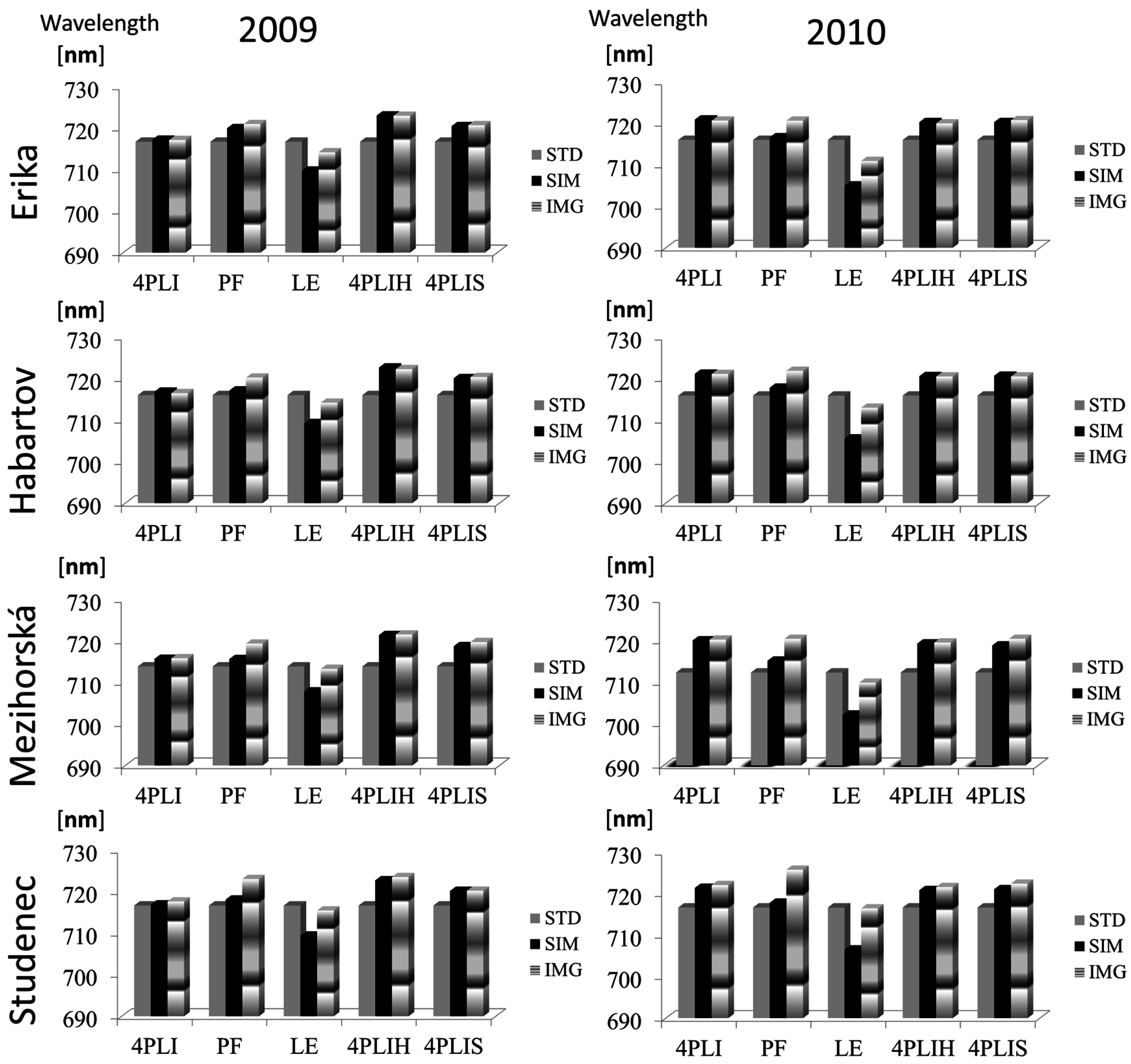
3.1. Comparison of REP_STD, REP_IMG and REP_SIM Values

The REP_STD was compared with REP_SIM and the corresponding REP_IMG at both the HyMap (5-m spatial resolution, PF, LE, 4PLI and 4PLIH methods) and S2 (20-m spatial resolution, 4PLIS method) levels (Figure 3). The relative fitting of the REP_IMG and REP_SIM can be considered satisfactory. A considerable difference can be seen between the REP_SIM and REP_IMG spectra when using the LE extraction method followed by the PF algorithm at all the study sites for both years (2009 and 2010).

Table 1. Comparison of RMSE and R² values of REP_SIM and REP_IMG (Calculated by 4PLI, PF, LE, 4PLIH and 4PLIS methods).

Method	Year	RMSE (nm)	R2
4PLI	2009	0.45	0.66
	2010	0.43	0.74
PF	2009	3.51	0.28
	2010	5.57	0.48
LE	2009	5.25	0.49
	2010	7.88	0.71
4PLIH	2009	0.42	0.66
	2010	0.38	0.74
4PLIS	2009	0.75	0.67
	2010	1.11	0.69

lists the RMSE values which describe the difference between the REP_SIM and REP_IMG values as well as R², which explains the correlation between the REP_IMG and REP_SIM values obtained by applying various REP extraction methods in both years (2009 and 2010).

The obtained results showed that the best fit (characterized by the lowest RMSE together with the highest R²) between the REP_IMG and REP_SIM values was found when using the 4PLI extraction method (RMSE₂₀₀₉ = 0.45 nm, R²₂₀₀₉ = 0.66; RMSE₂₀₁₀ = 0.43 nm, R²₂₀₁₀ = 0.74) and its 4PLIH version optimized specifically for the HyMap dataset (RMSE₂₀₀₉ = 0.42 nm, R²₂₀₀₉ = 0.66; RMSE₂₀₁₀ = 0.38 nm, R²₂₀₁₀ = 0.74). The 4PLIS method optimized for S2 data yielded results, which are generally comparable with its hyperspectral versions 4PLI or 4PLIH, although the RMSE value was slightly higher in this case (RMSE₂₀₀₉ = 0.75 nm, R²₂₀₀₉ = 0.67; RMSE₂₀₁₀ = 1.11 nm, R²₂₀₁₀ = 0.69).

Both the REP_IMG and REP_SIM values were compared with the REP_STD values. The differences between the REP_IMG (or REP_SIM) values and the corresponding REP_STD values (REP_SIM/STD and REP_IMG/STD respectively) were expressed by RMSE and R². Both RMSE and R² values for 2009 and 2010 can be found in

Table 2. Comparison of RMSE and R² values of REP_SIM/STD and REP_IMG/STD (For HyMap: 4PLI, PF, LE, 4PLIH and for simulated S2 data: 4PLIS methods).

Method	Year	Data	RMSE (nm)	R2
4PLI	2009	REPSIM/STD	5.14	0.96
		REPIMG/STD	5.31	0.81
	2010	REPSIM/STD	5.76	0.96
		REPIMG/STD	5.92	0.56
PF	2009	REPSIM/STD	6.04	0.75
		REPIMG/STD	6.15	0.56
	2010	REPSIM/STD	7.81	0.83
		REPIMG/STD	7.15	0.37
LE	2009	REPSIM/STD	6.78	0.92
		REPIMG/STD	6.71	0.62
	2010	REPSIM/STD	10.42	0.86
		REPIMG/STD	7.18	0. 53
4PLIH	2009	REPSIM/STD	5.02	0.96
		REPIMG/STD	5.13	0.81
	2010	REPSIM/STD	6.64	0.96
		REPIMG/STD	6.76	0.56
4PLIS	2009	REPSIM/STD	4.06	0.98
		REPIMG/STD	4.73	0.81
	2010	REPSIM/STD	5.05	0.96
		REPIMG/STD	6.11	0.52

.

Comparison of REP_SIM/RE_IMG values with REP_STD yielded following results. For the REP_SIM/STD values, the best fit was found for 4PLI and PLIH (the same R²; however RMSE are generally higher for the 2010 dataset). For the PF and LE methods, lower R² and higher RMSE were achieved; in addition, much higher deviations between REP_SIM/STD and REP_IMG/STD were found. Furthermore, comparable results with those derived for HyMap (4PLI and PLIH) were achieved for simulated S2 data when employing the (4PLIS) method. The RMSE values obtained for the 2010 dataset were generally higher compared with the ones obtained from the 2009 dataset. This can be explained by a higher signal-to-noise-ratio (SNR), which characterized the 2009 HyMap dataset when compared to the 2010 HyMap data [60].

The REP values were then extracted from the HyMap imagery as well as from the simulated S2 image data using the 4PLIH and 4PLIS methods (Figure 4). The results displayed in Figure 4 show that the REP spatial gradients are in good agreement when using HyMap (5-m spatial resolution) and simulated S2 image data (20-m spatial resolution). In addition, The HyMap REP image was resampled to 20-m spatial resolution to be spatially comparable with the S2 level data and to be able to display a scatterplot between the REP values extracted from HyMap and simulated S2 datasets (Figure 5).

The scatterplot of the REP values extracted from the HyMap and simulated S2 datasets suggested that the difference between these two datasets had a linear character with a systematic offset (Figure 5).

3.2. Correlation of the REP Calculated by Different Methods with Chl × LAI Values

The REP values obtained by the described extraction methods were correlated with the corresponding Chl × LAI content. The R² of REP_SIM-Chl × LAI and REP_IMG-Chl × LAI are listed in

Table 3. R² and RMSE describing the relationship of the REP_SIM/REP_IMG and Chl × LAI values.

Method	Year	REPSIM	REPIMG
		Chl × LAI	Chl × LAI
HyMap Level
4PLI	2009	0.72 (RMSE: 35.99 mg/m2)	0.58 (RMSE: 44.05 mg/m2)
	2010	0.49 (RMSE 40.12 mg/m2)	0.67 (RMSE: 32.04 mg/m2)
PF	2009	0.91 (RMSE: 5.99 mg/m2)	0.30 (RMSE: 57.26 mg/m2)
	2010	0.28 (RMSE: 47.61 mg/m2)	0.61 (RMSE: 34.46 mg/m2)
LE	2009	0.74 (RMSE: 35.13 mg/m2)	0.22 (RMSE: 60.27 mg/m2)
	2010	0.51 (RMSE: 39.21 mg/m2)	0.61 (RMSE: 34.98 mg/m2)
4PLIH	2009	0.72 (RMSE: 35.99 mg/m2)	0.58 (RMSE: 44.05 mg/m2)
	2010	0.49 (RMSE: 40.12 mg/m2)	0.67 (RMSE: 32.04 mg/m2)
Sentinel-2 Level
4PLIS	2009	0.71 (RMSE: 36.61 mg/m2)	0.48 (RMSE: 49.28 mg/m2)
	2010	0.48 (RMSE: 40.60 mg/m2)	0.67 (RMSE: 32.11 mg/m2)

.

The R² obtained for REP_IMG-Chl × LAI ranged from 0.22 to 0.67. The most consistent results when compared REP_IMG-Chl × LAI and REP_SIM-Chl × LAI as well as the highest correlations between HyMap REP_IMG and the Chl × LAI values were obtained using the 4PLI extraction method or its derivatives 4PLIH (Chl × LAI: RMSE₂₀₀₉ = 44.05 mg/m², RMSE₂₀₁₀ = 32.04 mg/m²). Employing the 4PLIS method, comparable correlation levels with those derived for HyMap were obtained between the simulated S2 REP_IMG and Chl × LAI (Chl × LAI: RMSE₂₀₀₉ = 49.28 mg/m², RMSE₂₀₁₀ = 32.11 mg/m²).

4. Discussion

This study modelled the REP for a Norway spruce Forest canopy Reflectance and Transmittance (FRT) using RTM (resampled to HyMap and S2 spectral resolution) as well as calculated the REP from the real HyMap and simulated S2 data. The S2 data were simulated from the HyMap 2009 and 2010 datasets using the forward and backward simulation modules (S2eteS) [47]; during this transformation, the effect of the real atmosphere was added to the image data as well as the real property of the sensor (e.g., sensor noise and detector nonlinearity). Therefore, this approach allowed a close-to-real sensor simulation of the S2 data, rather than just simple spectral and spatial resampling.

The REP was calculated using the following methods: PF, LE and 4PLI and its optimized versions for the spectral setting of the HyMap (4PLIH) and S2 data (4PLIS). The REP values calculated from image-extracted spectra (REP_IMG) were compared with the REP values extracted from canopy spectra simulated by couplings of PROSPECT-5 and FRT RTMs (REP_SIM) as well as with the comparative standard (REP_STD). The best match between HyMap REP_IMG and both REP_SIM and REP_STD was found in the case of the 4PLI method and the optimized version (4PLIH). Furthermore, comparable results with those derived for HyMap, were achieved for simulated S2 data when employing the (4PLIS) method to extract the REP. The deviations between the REP_SIM and REP_IMG can be caused by the following factors. Unlike the PROSPECT-5-simulated data, the image datasets, HyMap and simulated Sentinel-2, both contain noise (HyMap because it is a real aerial hyperspectral dataset and the simulated S2 data because sensor noise was added as well as the parameters of the atmosphere). Moreover, the leaf internal structure considered by this model does not match the real structure of coniferous needles [59]. Consequently, there might be some differences between the measured needle spectra and the model simulated ones. These differences are then propagated through the shoot and canopy up-scaling process, which can result in a mismatch between the model-simulated and image-extracted vegetation spectra. In general, a better fit between REP_IMG and REP_SIM and REP_STD (higher R² and lower RMSE) for both HyMap and the simulated S2 image data was found for the 2009 dataset when compared to the 2010 dataset. This can be explained by the higher signal-to-noise-ratio (SNR), which characterized the 2009 HyMap dataset [60].

When correlating the REP extracted from hyMap data using the above-mentioned methods with the Chl × LAI content, the highest R² were obtained using the 4PLI method together with its optimized versions (4PLIH). Furthermore, comparable correlation levels were obtained between the Chl × LAI and REP derived from the HyMap employing 4PLIH and the simulated S2 data when employing the 4PLIS. A similar trend was demonstrated by Delegido et al. [35] in the study employed over diverse agriculture sites. The Chl × LAI maps were derived for simulated S2 data and aerial Airborne Hyperspectral System (AHS) data employing the Normalized Area Over the reflectance Curve (NAOC) method. It was demonstrated that the estimated chlorophyll from simulated S2 image was practically the same as the one estimated from the original AHS image. Similarly, Clevers and Gitelson [39] demonstrated the significance of the red-edge bands of S2 sensor for estimation Chl content in crops and grasslands. These results show that due to the inclusion of red-edge bands, S2 has a great potential for delivering high-quality products (e.g., estimates of chlorophyll content).

The spatial resolution of either the HyMap (5-m spatial resolution) or S2 image data (20-m spatial resolution) did not allow a direct comparison between the sampling tree-tops and corresponding pixel values. Instead, it was possible to compare the tree groups/clusters with corresponding ROI’s pixel groups of HyMap and simulated S2 data. To be able to obtain comparable statistical results, the same ROIs were used for both HyMap and S2 statistics. This clustering decreased the number of the available input data for the empirical modelling of Chl × LAI. As a result, the Chl sampling points were averaged per site as well as the REP values from the pixels falling within the ROI’s (in total 4 sites were evaluated). On the other hand, the authors believe that it helped to minimize the errors resulting from false identifications between sampled tree-tops and corresponding pixels. Moreover, the values were more representative due to them being an average of 10–15 sampled trees. No strong statistical conclusions can be made using this limited dataset; however, the results demonstrate that the S2 REP is a promising tool for mapping Chl gradients and their spatial trends when assessing forests. However, further research focusing on the utilization of S2 REP to estimate forest biochemical parameters, which would also include an extensive validation campaign, is still needed and remains a challenge for the future.

The next step should also include testing new retrieval algorithms. As suggested by Delegido et al. [35], it would be interesting to apply and evaluate advanced non-parametric statistical models to S2 data, more sophisticated regression methods (e.g., stepwise multiple linear regression, principal component regression, partial least square regression [61,62] and new machine learning techniques such as Gaussian processes regression [63,64,65,66]. However, to employ, evaluate and validate these techniques much more extensive input data and ground truth datasets are required, especially for forests.

5. Conclusions

In this forest-oriented study, it was demonstrated that it is possible to calculate the red-edge-position (REP) using the simulated Sentinel-2 (S2) image data with comparable accuracy when using HyMap hyperspectral data. The lowest differences in REP values calculated from image-extracted spectra and from theoretical RTM simulations were found for the 4PLI method including its HyMap (4PLIH) and S2 optimized versions (4PLIS). When assessing correlation levels between REP and the Chl × LAI contents the optimal solutions, in the case of HyMap, were found to be the 4PLI and 4PLIH methods and for simulated S2 image data the 4PLIS method. A comparable correlation level between REP and Chl × LAI was obtained when using simulated S2 image data despite their lower spatial and spectral resolution compared to airborne hyperspectral imagery, such as the HyMap data. Despite its simplicity, the 4PLI REP extraction technique demonstrated its potential usefulness for forest assessment based on both airborne hyperspectral (e.g., HyMap) as well as the space-borne S2 image data. Although S2 data have neither such high spatial nor spectral resolution as the data provided by current airborne hyperspectral sensors, they will make a major contribution to remote-sensing-based vegetation studies, especially because of their remarkably high temporal resolution and spatial coverage.

So far there are still very few studies devoted to the use of S2 data for estimating forest biochemistry/biophysics. These results demonstrate that the S2 REP has a potential to estimate chlorophyll gradients and to map spatial trends when assessing forests. However, further research focusing on the use of S2 REP to estimate forest biochemical parameters, which would also include an extensive validation campaign, is still needed and remains a challenge for the future.

References

1. Carter, G.A.; Knapp, A.K. Leaf optical properties in higher plants: Linking spectral characteristics to stress and chlorophyll concentration. Am. J. Bot. 2001, 88, 677–684. [Google Scholar] [CrossRef] [PubMed]
2. Pastor-Guzman, J.; Atkinson, P.M.; Dash, J.; Rioja-Nieto, R. Spatiotemporal variation in Mangrove chlorophyll concentration using Landsat 8. Remote Sens. 2015, 7, 14530–14558. [Google Scholar] [CrossRef]
3. Peñuelas, J.; Filella, I. Visible and near-infrared reflectance techniques for diagnosing plant physiological status. Trends Plant. Sci. 1998, 3, 151–156. [Google Scholar] [CrossRef]
4. Saberioon, M.M.; Amin, M.S.M.; Gholizadeh, A.; Ezrin, M.H. A review of optical methods for assessing nitrogen contents during rice growth. Appl. Eng. Agric. 2014, 30, 657–669. [Google Scholar]
5. Mišurec, J.; Kopačková, V.; Lhotáková, Z.; Hanus, J.; Weyermann, J.; Campbell, P.E.; Albrechtová, J. Utilization of hyperspectral image optical indices to assess the Norway spruce forest health status. J. Appl. Remote Sens. 2012, 6, 063545. [Google Scholar] [CrossRef]
6. Darvishzadeh, R.; Atzberger, C.; Skidmore, A.K.; Abkar, A.A. Leaf area index derivation from hyperspectral vegetation indices and the red edge position. Int. J. Remote Sens. 2009, 30, 6199–6218. [Google Scholar] [CrossRef]
7. Cho, M.A.; Skidmore, A.K. A new technique for extracting the red edge position from hyperspectral data: The linear extrapolation method. Remote Sens. Environ. 2006, 101, 181–193. [Google Scholar] [CrossRef]
8. Jacquemoud, S.; Baret, F. PROSPECT: A model of leaf optical properties spectra. Remote Sens. Environ. 1990, 34, 75–91. [Google Scholar] [CrossRef]
9. Jacquemoud, S.; Verhoef, W.; Baret, F.; Cédric, B.; Zarco-Tejada, P.J.; Asner, G.P.; Francois, C.; Ustin, S.L. PROSPECT + SAIL models: A review of use for vegetation characteristics. Remote Sens. Environ. 2009, 113, S56–S66. [Google Scholar] [CrossRef]
10. Ganapol, B.D.; Johnson, L.F.; Hammer, P.D.; Hlavka, C.A.; Peterson, D.L. A new within-leaf radiative transfer model. Remote Sens. Environ. 1998, 63, 182–193. [Google Scholar] [CrossRef]
11. Verhoef, W. Light-scattering by leaf layers with application to canopy reflectance modelling—The SAIL model. Remote Sens. Environ. 1984, 16, 125–141. [Google Scholar] [CrossRef]
12. Van der Tol, C.; Verhoef, W.; Timmermans, J.; Verhoef, A.; Su, Z. An integrated model of soil-canopy spectral radiance observations, photosynthesis, fluorescence, temperature and energy balance. Biogeosci. Discuss. 2009, 6, 6025–6075. [Google Scholar] [CrossRef]
13. Demarez, V.; Gastellu-Etchegorry, J.P. A modeling approach for studying forest chlorophyll content. Remote Sens. Environ. 2000, 71, 226–238. [Google Scholar] [CrossRef]
14. Jacquemoud, S. Inversion of the PROSPECT + SAIL canopy reflectance model from AVIRIS equivalent spectra: Theoretical study. Remote Sens. Environ. 1993, 44, 281–292. [Google Scholar] [CrossRef]
15. Chaurasia, S.; Dadhwal, V.K. Comparison of principal component inversion with VI-empirical approach for LAI estimation using simulated reflectance data. Int. J. Remote Sens. 2004, 25, 2881–2887. [Google Scholar] [CrossRef]
16. Clevers, J.G.P.W.; de Jong, S.M.; Epema, G.F.; van der Meer, F.; Bakker, W.; Skidmore, A.K. Derivation of the red edge index using MERIS standard band setting. Int. J. Remote Sens. 2002, 23, 3169–3184. [Google Scholar] [CrossRef]
17. Curran, P.J.; Windham, W.R.; Gholz, H.L. Exploring the relationship between reflectance red edge and chlorophyll concentration in slash pine leaves. Tree Physiol. 1995, 15, 203–206. [Google Scholar] [CrossRef] [PubMed]
18. Dawson, T.P.; Curran, P.J. A new technique for interpolating the reflectance red edge position. Int. J. Remote Sens. 1998, 19, 2133–2139. [Google Scholar] [CrossRef]
19. Buschmann, C.; Nagel, E. In vivo spectroscopy and internal optics of leaves as basis for remote sensing of vegetation. Int. J. Remote Sens. 1993, 14, 711–722. [Google Scholar] [CrossRef]
20. Boochs, F.; Kupfer, G.; Dockter, K.; Kuhbauch, W. Shape of the red-edge as vitality indicator for plants. Int. J. Remote Sens. 1990, 11, 1741–1753. [Google Scholar] [CrossRef]
21. Gates, D.M.; Keegan, H.J.; Schleter, J.C.; Weidner, V.R. Spectral properties of plants. Appl. Opt. 1965, 4, 11–20. [Google Scholar] [CrossRef]
22. Horler, D.N.H.; Dockray, M.; Barber, J. The red edge of plant leaf reflectance. Int. J. Remote Sens. 1983, 4, 273–288. [Google Scholar] [CrossRef]
23. Ramoelo, A.; Skidmore, A.K.; Cho, M.A.; Schlerf, M.; Mathieu, R.; Heitkönig, I.M.A. Regional estimation of savanna grass nitrogen using the red-edge band of the spaceborne rapideye sensor. Int. J. Appl. Earth Obs. Geoinform. 2012, 19, 151–162. [Google Scholar] [CrossRef]
24. Verrelst, J.; Camps-Valls, G.; Muñoz-Marí, J.; Rivera, J.P.; Veroustraete, F.; Clevers, J.G.P.W.; Moreno, J.J. Optical remote sensing and the retrieval of terrestrial vegetation bio-geophysical properties—A review. ISPRS J. Photogramm. Remote Sens. 2015, 108, 273–290. [Google Scholar] [CrossRef]
25. Description of Derivative-Based High Spectral-Resolution (AVIRIS) Green Vegetation Index. Available online: http://proceedings.spiedigitallibrary.org/proceeding.aspx?articleid=1011206 (accessed on 8 October 2016).
26. Demetriades-Shah, T.H.; Steven, M.D.; Clark, J.A. High resolution derivative spectra in remote sensing. Remote Sens. Environ. 1990, 33, 55–64. [Google Scholar] [CrossRef]
27. Railyan, V.Y.; Korobov, R.M. Red edge structure of canopy refectance spectra of triticale. Remote Sens. Environ. 1993, 46, 173–182. [Google Scholar] [CrossRef]
28. Savitzky, A.; Golay, M.J.E. Smoothing and differentiation of data by simplified least squares procedures. Anal. Chem. 1964, 36, 1627–1639. [Google Scholar] [CrossRef]
29. Pu, R.; Gong, P.; Biging, G.S.; Larrieu, M.R. Extraction of red edge optical parameters from Hyperion data for estimation of forest leaf area index. IEEE Trans. Geosci. Remote Sens. 2003, 41, 916–921. [Google Scholar]
30. Hare, E.W.; Miller, J.R.; Hollinger, A.B.; Sturgeon, D.R.; O’Neil, N.T.; Ward, T.V. Measurements of the vegetation reflectance red edge with an airborne programmable imaging spectrometer. In Proceedings of the Fifth Thematic Conference on Remote Sensing For Exploration Geology, Reno, NV, USA, 29 October 1986; Environmental Institute of Michigan: Ann Arbor, MI, USA; p. 657.
31. Frampton, W.J.; Dash, J.; Watmough, G.; Milton, E.J. Evaluating the capabilities of Sentinel-2 for quantitative estimation of biophysical variables in vegetation. ISPRS J. Photogramm. Remote Sens. 2013, 82, 83–92. [Google Scholar] [CrossRef]
32. Dotzler, S.; Hill, J.; Buddenbaum, H.; Stoffels, J. The potential of EnMAP and Sentinel-2 data for detecting drought stress phenomena in deciduous forest communities. Remote Sens. 2015, 7, 14227–14258. [Google Scholar] [CrossRef]
33. Laurin, G.V.; Puletti, N.; Hawthorne, W.; Liesenberg, V.; Corona, P.; Papale, D.; Chen, Q.; Valentini, R. Discrimination of tropical forest types, dominant species, and mapping of functional guilds by hyperspectral and simulated multispectral Sentinel-2 data. Remote Sens. Environ. 2016, 176, 163–176. [Google Scholar] [CrossRef] [Green Version]
34. Verrelst, J.; Rivera, J.P.; Veroustraete, F.; Muñoz-Marí, J.; Clevers, J.G.P.W.; Camps-Valls, G.; Moreno, J.J. Experimental Sentinel-2 LAI estimation using parametric, non-parametric and physical retrieval methods—A comparison. ISPRS J. Photogramm. Remote Sens. 2015, 108, 260–272. [Google Scholar] [CrossRef]
35. Delegido, J.; Verrelst, J.; Alonso, L.; Moreno, J. Evaluation of Sentinel-2 red-edge bands for empirical estimation of green LAI and chlorophyll content. Sensors 2011, 11, 7063–7081. [Google Scholar] [CrossRef] [PubMed]
36. Atzberger, C.; Richter, K. Spatially constrained inversion of radiative transfer models for improved LAI mapping from future Sentinel-2 imagery. Remote Sens. Environ. 2012, 120, 208–218. [Google Scholar] [CrossRef]
37. Richter, K.; Atzberger, C.; Vuolo, F.; Weihs, P.; D’Urso, G. Experimental assessment of the Sentinel-2 band setting for RTM-based LAI retrieval of sugar beet and maize. Can. J. Remote Sens. 2009, 35, 230–247. [Google Scholar] [CrossRef]
38. Richter, K.; Hank, T.B.; Vuolo, F.; Mauser, W.; D’Urso, G. Optimal exploitation of the Sentinel-2 spectral capabilities for crop leaf area index mapping. Remote Sens. 2012, 4, 561–582. [Google Scholar] [CrossRef] [Green Version]
39. Clevers, J.G.P.W.; Gitelson, A.A. Remote estimation of crop and grass chlorophyll and nitrogen content using red-edge bands on Sentinel-2 and -3. Int. J. Appl. Earth Obs. Geoinform. 2013, 23, 344–351. [Google Scholar] [CrossRef]
40. Verrelst, J.; Munoz, J.; Alonso, L.; Delegido, J.; Rivera, J.P.; Camps-Valls, G.; Moreno, J. Machine learning regression algorithms for biophysical parameter retrieval: Opportunities for Sentinel-2 and -3. Remote Sens. Environ. 2012, 118, 127–139. [Google Scholar] [CrossRef]
41. Delegido, J.; Verrelst, J.; Meza, C.M.; Rivera, J.P.; Alonso, L.; Moreno, J. A red-edge spectral index for remote sensing estimation of green LAI over agroecosystems. Eur. J. Agron. 2013, 46, 42–52. [Google Scholar] [CrossRef]
42. Schlerf, M.; Atzberger, C.; Hill, J. Remote sensing of forest biophysical variables using HyMap imaging spectrometer data. Remote Sens. Environ. 2005, 95, 177–194. [Google Scholar] [CrossRef]
43. Fernández-Manso, A.; Fernández-Manso, O.; Quintano, C. SENTINEL-2A red-edge spectral indices suitability for discriminating burn severity. Int. J. Appl. Earth Obs. Geoinform. 2016, 50, 170–175. [Google Scholar] [CrossRef]
44. Kopačková, V.; Mišurec, J.; Lhotáková, Z.; Oulehle, F.; Albrechtová, J. Using multi-date high spectral resolution data to assess the physiological status of macroscopically undamaged foliage on a regional scale. Int. J. Appl. Earth Obs. Geoinform. 2014, 27, 169–186. [Google Scholar] [CrossRef]
45. Hu, B.; Lucht, W.; Li, X.; Strahler, A.H. Validation of kernel-driven models for the BRDF of land surfaces. Remote Sens. Environ. 1997, 62, 201–214. [Google Scholar] [CrossRef]
46. Schaaf, C.; Gao, F.; Strahler, A.; Lucht, W.; Li, X.; Tsang, T.; Strugnell, N.; Zhang, X.; Jin, Y.; Muller, J.P.; et al. First operational BRDF, Albedo and nadir reflectance products from MODIS. Remote Sens. Environ. 2002, 83, 135–148. [Google Scholar] [CrossRef]
47. Segl, K.; Guanter, L.; Gascon, F.; Kuester, T.; Rogass, C.; Mielke, C. S2eteS: An end-to-end modeling tool for simulation of S2image products. IEEE Trans. Geosci. Remote Sens. 2015, 53, 5560–5571. [Google Scholar] [CrossRef]
48. Mielke, C.; Boesche, N.K.; Rogass, C.; Segl, K.; Gauert, C.; Kaufmann, H. Potential applications of the Sentinel-2 multispectral sensor and the EnMap hyperspectral sensor in mineral exploration. EARSeL eProc. 2014, 13, 93–102. [Google Scholar]
49. Porra, R.J.; Thompson, W.A.; Kriedemann, P.E. Determination of accurate extinction coefficients and simultaneous equations for assaying chlorophylls a and b extracted with four different solvents: Verification of the concentration of chlorophyll standards by atomic absorption spectrometry. Biochim. Biophys. Acta 1989, 975, 384–394. [Google Scholar] [CrossRef]
50. Wellburn, A.R. The spectral determination of chlorophyll a and b, as well as total carotenoids, using various solvents with spectrophotometers of different resolution. J. Plant Physiol. 1994, 144, 307–313. [Google Scholar] [CrossRef]
51. Homolová, L.; Malenovský, Z.; Clevers, J.G.P.W.; García-Santos, G.; Schaepman, M.E. Review of optical-based remote sensing for plant trait mapping. Ecol. Complex. 2013, 15, 1–16. [Google Scholar] [CrossRef]
52. Lhotáková, Z.; Brodský, L.; Kupková, L.; Kopačková, V.; Potůčková, M.; Mišurec, J.; Klement, A.; Kovářová, M.; Albrechtová, J. Detection of multiple stresses in Scots pine growing at post-mining sites using visible to near-infrared spectroscopy. J. Environ. Monit. 2013, 15, 2004–2015. [Google Scholar]
53. Féret, J.B.; François, C.; Asner, G.P.; Gitelson, A.A.; Martin, R.E.; Bidel, L.P.R.; Ustin, S.L.; le Maire, G.; Jacquemoud, S. PROSPECT-4 and 5: Advances in the leaf optical properties model separating photosynthetic pigments. Remote Sens. Environ. 2008, 112, 3030–3043. [Google Scholar] [CrossRef]
54. Zarco-Tejada, P.J.; Miller, J.R. Land cover mapping at BOREAS using red edge spectral parameters from CASI imagery. J. Geophys. Res. 1999, 104, 27921–27933. [Google Scholar] [CrossRef]
55. Rautiainen, M.; Mõttus, M.; Yáñez-Rausell, L.; Homolová, L.; Malenovský, Z.; Schaepman, M.E. A note on upscaling coniferous needle spectra to shoot spectral albedo. Remote Sens. Environ. 2012, 117, 469–474. [Google Scholar] [CrossRef]
56. Knyazikhin, Y.; Schull, M.A.; Xu, L.; Myneni, R.B.; Samanta, A. Canopy spectral invariants. Part 1: A new concept in remote sensing of vegetation. J. Quant. Spectrosc. Radiat. Transf. 2011, 112, 727–735. [Google Scholar] [CrossRef]
57. Huang, D.; Knyazikhin, Y.; Dickinson, R.E.; Rautiainen, M.; Stenberg, P.; Disney, M.; Lewis, P.; Cescatti, A.; Tian, Y.; Verhoef, W.; et al. Canopy spectral invariants for remote sensing and model applications. Remote Sens. Environ. 2007, 106, 106–122. [Google Scholar] [CrossRef]
58. Kuusk, A.; Nilson, T. A directional multispectral forest reflectance model. Remote Sens. Environ. 2000, 72, 244–252. [Google Scholar] [CrossRef]
59. Allometric Relationships of Selected European Tree Species. Available online: http://publications.jrc.ec.europa.eu/repository/bitstream/JRC26286/EUR%2020855%20EN.pdf (accessed on 28 September 2016).
60. Bachmann, M.; Richter, R.; Holzwarth, S.; Weide, S.; Fischer, C.; Ehrler, C. Quality Report on HyMap 2009 Sokolov Data; Internal Report of the EO-MINERS Project, DLR; DLR’s Research Center Oberpfaffenhofen: Bavaria, Germany, 2011; pp. 1–25. [Google Scholar]
61. Glenn, E.P.; Huete, A.R.; Nagler, P.L.; Nelson, S.G. Relationship between remotely-sensed vegetation indices, canopy attributes and plant physiological processes: What vegetation indices can and cannot tell us about the landscape. Sensors 2008, 8, 2136–2160. [Google Scholar] [CrossRef]
62. Darvishzadeh, R.; Skidmore, A.; Schlerf, M.; Atzberger, C.; Corsi, F.; Cho, M. LAI and chlorophyll estimation for a heterogeneous grassland using hyperspectral measurements. ISPRS J. Photogramm. Remote Sens. 2008, 63, 409–426. [Google Scholar] [CrossRef]
63. Verrelst, J.; Alonso, L.; Camps-Valls, G.; Delegido, J.; Moreno, J. Retrieval of canopy parameters using gaussian processes techniques. IEEE Trans. Geosci. Remote Sens. 2011. [Google Scholar] [CrossRef]
64. Smola, J.; Schölkopf, B. A tutorial on support vector regression. Stat. Comput. 2004, 14, 199–222. [Google Scholar] [CrossRef]
65. Camps-Valls, G.; Bruzzone, L.; Rojo-Alvarez, J.L.; Melgani, F. Robust support vector regression for biophysical variable estimation from remotely sensed images. IEEE Geosci. Remote Sens. Lett. 2006, 3, 339–343. [Google Scholar] [CrossRef]
66. Baret, F.; Hagolle, O.; Geiger, B.; Bicheron, P.; Miras, B.; Huc, M.; Berthelot, B.; Niño, F.; Weiss, M.; Samain, O.; et al. LAI, fAPAR and fCover CYCLOPES global products derived from VEGETATION: Part 1: Principles of the algorithm. Remote Sens. Environ. 2007, 110, 275–286. [Google Scholar] [CrossRef] [Green Version]
Figure 1. Location of the Sokolov lignite basin in the western part of the Czech Republic. Four sampled Norway spruce stands: Erika (E), Habartov (H), Mezihorská (M) and Studenec (S). Background map © ČUZK.
Forests 07 00226 g001
Figure 2. Example (the Mezihorská site) showing the Regions Of Interest (ROI) and the sampling points overlaid on the hyMap (left) and simulated Sentinel 2 (right). At the top: per-ROI-averaged reflectance derived for HyMap (left) and simulated S2 image data (right) which was used in the following analyses.
Forests 07 00226 g002
Figure 3. REP averages per sites: The REPSTD compared with REPSIM and the corresponding REPIMG at both the HyMap (5-m spatial resolution, PF, LE, 4PLI and PLIH methods) and S2 (20-m spatial resolution, 4PLIS method) levels.
Forests 07 00226 g003
Figure 4. REP calculated from the 2009 (a) HyMap hyperspectral dataset (5-m spatial resolution) and (b) simulated S2 (20-m spatial resolution) dataset.
Forests 07 00226 g004
Figure 5. Scatterplot of the REP values extracted from HyMap data (20-m spatial resolution) and simulated S2 dataset (20-m spatial resolution).
Forests 07 00226 g005