Article

Scale-Dependent Stand Spatial Structure and Crown Competition in a Subtropical Mixed Forest Based on Individual-Tree Spatial Data

School of Computer Science and Mathematics, Central South University of Forestry and Technology, Changsha 410004, China
*
Author to whom correspondence should be addressed.
Forests 2026, 17(9), 1124; https://doi.org/10.3390/f17091124
Submission received: 3 July 2026 / Revised: 30 August 2026 / Accepted: 18 September 2026 / Published: 20 September 2026
(This article belongs to the Section Forest Inventory, Modeling and Remote Sensing)

Abstract

Background and Objectives: Aggregating mapped trees into larger cells necessarily reduces some among-cell variation; ecological scale responses must therefore be distinguished from arithmetic averaging. We evaluated stand structure and crown competition across spatial grains and tested whether the observed spatial contrast exceeded a fixed-pattern random-label benchmark. Materials and Methods: A mapped inventory from Nanshan Nature Reserve, Hunan Province, China, contained 114,524 cleaned stems (DBH ≥ 1.0 cm) from 297 recorded species over approximately 24 ha. Four-nearest-neighbor structural indices, Hegyi competition ( C I ), crown-width distance competition ( C C I ), and circular crown overlap ( C O I ) were calculated for every stem and summarized in 5–50 m grids. The analyses included 199 random-label permutations, pair- and mark-correlation functions, 50 m spatial-block bootstrap resampling, and a complete reanalysis restricted to DBH ≥ 5 cm. Results: At 20 m, the observed among-cell coefficients of variation for Hegyi, C O I , and mingling were 2.31, 8.73, and 3.24 times their random-label medians, respectively, whereas crown occupancy was below its null envelope. Hegyi exceeded the 95% null envelope at fine and intermediate grains but not at 40 or 50 m, where few cells remained. Pair correlation exceeded one from 0 to 20 m under both DBH thresholds, and conspecific association was strongest at short distances. As expected from the DBH-based crown model, C C I was strongly associated with Hegyi at tree level ( ρ s = 0.953 ), whereas C O I was less strongly associated ( ρ s = 0.236 ). At 20 m, spatial-block bootstrap intervals were 0.818–0.878 for Hegyi– C C I and 0.294–0.484 for Hegyi– C O I . Reanalysis of 38,128 stems with DBH ≥ 5 cm preserved rank patterns but changed local Hegyi hotspot membership (Jaccard similarity 0.222); C O I hotspots were more stable (0.658). Conclusions: Fine and intermediate grains retained spatially concentrated competition and mixing signals beyond arithmetic averaging, but no single grain was universally optimal. The results support 10–20 m units for local screening and 30–50 m units for broader summaries, with explicit attention to stem-size thresholds and coarse-grain uncertainty.

1. Introduction

Neighborhood indices of mixing, size status, and crowding, including the distance-dependent Hegyi kernel, are standard descriptions of stand spatial structure [1,2,3]. Their numerical values nevertheless change with the plot or cell in which they are computed. Structural-index estimates in a mature silver-birch stand changed with sample-plot size and shape [4]; plot size altered spatial-structure models for Sudanian woodland [5]; sampling-plot area changed the precision of structural indicators in old-growth stands [6]; and plot size together with the spatial pattern of the measured attribute affected inventory sampling efficacy [7]. Those papers compared discrete plot designs. They do not test whether among-cell contrast in one continuously mapped stand exceeds the decline produced by aggregating the same trees into larger cells. In a heterogeneous subtropical mixed forest that distinction matters, because a coarse mean can hide locally high competition or low mingling. We therefore held the mapped trees fixed and varied only the summary grain: a continuous 5–50 m grid, compared with a fixed-pattern random-label benchmark that keeps tree locations, cell counts, and each metric’s marginal distribution constant.
Crown width scales with stem size [8]. When crowns come from a DBH allometry, a distance-weighted crown-width ratio therefore retraces the Hegyi size ratio; independently measured crown geometry can instead record canopy crowding that diameters miss, as in overlap-based neighborhoods and UAV-LiDAR crown projection or volume [9,10]. The crown widths used here follow a calibrated DBH power law, so crown-width distance competition is treated as a sensitivity control, and the open question is whether circular crown overlap still varies after Hegyi is accounted for.
Distance-resolved functions such as the pair-correlation function g ( r ) describe how stems and marks cluster with distance [11]. Forest inventories more often encode the same structure as four-neighbor indices around a reference tree [1], including mapped mixed-forest plots [2] and GIS aggregations built for field decisions [12]. Finite maps still omit neighbors beyond the boundary [13]. This study therefore computes four-neighbor indices on the full mapped pattern and uses pair- and mark-correlation functions, with a DBH-threshold reanalysis, as a distance-resolved check of the same stems.
Most multi-scale structural assessments still rely on relatively small plots, a single metric family, or a few summary grains. Continuous hectare-scale inventories that jointly examine neighborhood structure, stem competition, and canopy crowding, while distinguishing aggregation artefacts from spatial concentration, remain uncommon in species-rich subtropical secondary forests. This study does not propose a new index. Instead, it develops and tests an inventory-scale workflow on an approximately 24 ha mapped stand: a continuous 5–50 m grain series for structural and competition summaries; a fixed-pattern random-label benchmark that separates spatial concentration from arithmetic averaging; pair- and mark-correlation diagnostics with a DBH-threshold reanalysis; and an explicit evaluation of which crown metrics complement Hegyi under the available crown model. The resulting interpretation links grain size to local screening and broader stand reporting without assuming a universally optimal plot size.
We therefore asked how structural and competition summaries change with grain; whether among-cell contrast exceeds random-label expectations after tree locations, cell counts, and metric marginal distributions are fixed; which crown metrics complement Hegyi under the present crown model; and how sensitive the results are to neighbor number, stem-size threshold, crown-width perturbation, cell filtering, and outer-boundary treatment.

2. Materials and Methods

This was a cross-sectional observational study of one continuously mapped forest stand. Tree-level structural and competition indices were summarized within fixed square cells. The primary scale comparison contrasted the observed among-cell coefficient of variation with a fixed-pattern random-label benchmark.

2.1. Study Site and Field Inventory

The study area was located in Nanshan Nature Reserve, Suining County, Shaoyang City, Hunan Province, China (26°24′22″–26°24′35″ N, 110°04′59″–110°05′21″ E). The area has a humid mid-subtropical monsoon climate, with a mean annual temperature of approximately 16.7 °C and mean annual precipitation of approximately 1300 mm. The vegetation is subtropical evergreen broad-leaved secondary forest. The principal recorded tree species included Castanopsis fargesii, Castanopsis tibetana, Rhododendron latoucheae, Lindera pulcherrima var. hemsleyana, and Dendropanax dentiger; planted or associated species included Cunninghamia lanceolata and Camellia oleifera. Elevation was approximately 800–1200 m a.s.l. (Figure 1).
The archived inventory comprised 30 plot groups of contiguous 20 m × 20 m units along a north–south transect (Table 1). Point-name prefixes identified 600 units, all of which remained after record-level quality control. Each stem record included a tree identifier, WGS84 longitude and latitude measured by RTK, a recorded species label, DBH, tree height, and calibrated or estimated crown width. The census threshold was DBH ≥ 1.0 cm. Unit-level and taxon-level summaries for this single forest type are given in Table 2; census dates, survey duration, and crew size were not recorded. The point-name field reconstructed the original 20 m units for structural-type classification; coordinate-based regular grids were used for the primary multi-scale analysis because their areas are directly comparable across grains.
After tree-level cleaning, 114,524 stems representing 297 distinct recorded species labels were available for spatial analysis (Table 1). The projected coordinate extent was approximately 600.4 m by 400.8 m (about 24 ha). Crown width in the archive followed a power-law DBH–crown-width model, C W = 1.4 · D B H 0.6 (DBH in cm and C W in m), with the height constraint C W ≤ 1.2 H . A subsample was calibrated from UAV orthophotos by NDVI thresholding and ray-based extraction. We used those calibrated widths as supplied. Because they nevertheless followed a DBH allometry, crown-area, crown-overlap, and crown-competition results were interpreted as calibrated crown-space indicators rather than independent field measurements of physical crown contact.

2.2. Data Cleaning and Coordinate Transformation

We compiled tree ID, longitude, latitude, species, DBH, height, crown-width, and crown-model metadata from the archive. Decimal longitude and latitude were used as the primary coordinates. Records with truncated decimal coordinates were recovered from the original degree-minute-second text where possible. Records with unrecoverable coordinates, non-positive DBH, height, or crown width, missing species, or exact duplicate rows were excluded. Non-identical records with repeated tree identifiers were retained but flagged because they could represent local numbering conflicts rather than duplicate trees. Extreme DBH, height, and crown-width values were screened using descriptive statistics and interquartile-range rules but were not removed solely for being extreme. The archive contained 328 records (0.29% of the cleaned data) with reported height below 1.3 m despite a DBH value; these records are physically inconsistent with conventional breast-height measurement and were flagged as source-data anomalies. They were retained for coordinate- and DBH-based analyses because no independent correction was available. Height did not enter any of the six focal neighborhood or competition indices; excluding these records from the height summary changed the overall mean height only from 6.091 to 6.105 m.
Geographic coordinates were projected to UTM Zone 49N (EPSG:32649) before any Euclidean distance was calculated. Subtracting the minimum projected x and y values produced a local metric system, which was then used for nearest-neighbor, competition, and crown-overlap calculations.

2.3. Multi-Scale Spatial Unit Construction

A spatial unit was defined as a fixed-area polygon used to summarize tree-level attributes: either a regular grid cell of side length s (m) or a field-defined 20 m inventory unit reconstructed from the point-name field. Two schemes were used. The four-digit point-name prefix supported structural-type classification, whereas coordinate-based regular grids formed the primary scale-dependent framework. Tree-level indices were aggregated in 5 m increments from 5 to 50 m. Cells containing fewer than 10 trees were excluded from among-cell CV and diversity summaries. With 297 recorded taxa, a cell of only a few stems cannot support a stable richness or evenness value, and the among-cell CV of such means is then dominated by empty-cell noise rather than stand structure. The N ≥ 10 rule therefore defines the summary, not the map: tree-level indices still use every stem, and the plotted grids still show the full layout. Replacing the threshold with N ≥ 5 or N ≥ 20 did not change the rank order of the grain series (Supplementary Table S6 and Figure S6). Under the primary N ≥ 10 rule, 5818, 2374, 601, 280, and 104 cells were retained at 5, 10, 20, 30, and 50 m, respectively; uncertainty therefore increased at coarse grains.

2.4. Stand Structural Attributes

For each spatial unit, we calculated tree count, species richness, means and standard deviations of DBH, height, and calibrated crown width, basal area, tree density, basal area per hectare, Shannon diversity, Simpson diversity, Pielou evenness, large-tree proportion (DBH ≥ 20 cm), small-tree proportion (DBH < 5 cm), total crown area, crown occupancy, and height-layer Shannon diversity. Species metrics used all cleaned stems with DBH ≥ 1.0 cm in the unit. For species proportions p s = n s / N , Shannon diversity was H ′ = − ∑ s p s ln p s [14]. Simpson concentration was λ = ∑ s p s 2 [15]; we report its plug-in complement, 1 − λ , as Simpson diversity. Pielou evenness was J ′ = H ′ / ln S for richness S > 1 [16]; we set J ′ = 0 when S = 1 . Basal area was calculated as B A i = π ( D B H i / 200 ) 2 , with DBH in cm and basal area in m2, and individual crown area was approximated as π ( C W i / 2 ) 2 . We defined crown occupancy as the sum of these study-defined circular crown areas divided by unit area. Because the numerator does not subtract overlapping crown area and crowns may occupy multiple vertical layers, crown occupancy may exceed 1; it is interpreted as relative crown-area load rather than planar canopy cover.

2.5. Neighborhood-Based Spatial Structure Indices

Nearest-neighbor searches were performed on the continuously mapped point pattern. For each focal tree i, the baseline analysis used its four nearest neighbors j = 1 , … , 4 to calculate species mingling, DBH-based neighborhood comparison, nearest-neighbor distance, mean four-neighbor distance, and the uniform-angle index. The four-neighbor choice for the uniform-angle index follows von Gadow et al. [17]; Aguirre et al. and Li et al. applied the same four-tree neighborhood to mingling and size-dominance variables in mixed forests [2,18]. We used k = 4 as the baseline and recalculated the indices with k = 6 and k = 8 to check rank stability. Neighbor searches were not restricted to individual grid cells, so artificial grid boundaries did not truncate four-neighbor sets. Formal definitions were as follows:
M i = 1 4 ∑ j = 1 4 v i j , v i j = 1 , if species of j ≠ species of i , 0 , otherwise .
U i = 1 4 ∑ j = 1 4 k i j , k i j = 1 , if D B H j > D B H i , 0 , otherwise .
W i = 1 4 ∑ j = 1 4 z i j ,
We set z i j = 1 when the angle between adjacent neighbor bearings was smaller than the simulation-derived standard angle of 72 ° , and z i j = 0 otherwise [19]. The indices are also summarized in Table 3.

2.6. Competition and Crown-Overlap Indices

Stem competition was calculated with a modified Hegyi index in which the original DBH-ratio/inverse-distance kernel [3] was evaluated over the four nearest neighbors, rather than over Hegyi’s original fixed-radius competitor set:
C I i = ∑ j = 1 4 D B H j / D B H i d i j ,
where d i j is the Euclidean distance (m) between focal tree i and neighbor j. To prevent division by zero for coincident coordinates, the minimum distance was set to 0.05 m. Crown-width distance competition was calculated analogously:
C C I i = ∑ j = 1 4 C W j / C W i d i j .
If C W ∝ D B H b in the absence of other constraints, then C W j / C W i = ( D B H j / D B H i ) b , so C C I is a monotonic transformation of the Hegyi size ratio. Under the power-law crown model used here ( b = 0.6 ), a strong association between C C I and C I was expected by construction. The height constraint and calibration residuals could introduce limited differences, but C C I was not interpreted as an independent crown metric.
For the study-defined crown-overlap index ( C O I ), each crown was approximated by a circle of radius C W / 2 . When d i j < r i + r j , we calculated the two-circle intersection area, summed the overlaps assigned to focal tree i, and divided by its circular crown area. Multiple neighbors may overlap the same focal crown, so C O I may exceed 1 and is interpreted as overlap load rather than unit-area cover. Candidate neighbors were identified by a radius search. Crown overlap can describe a functional neighborhood beyond stem size [9]; we estimated C O I on circular crowns and compared it with Hegyi in the Results Section.

2.7. Scale-Dependent Analysis

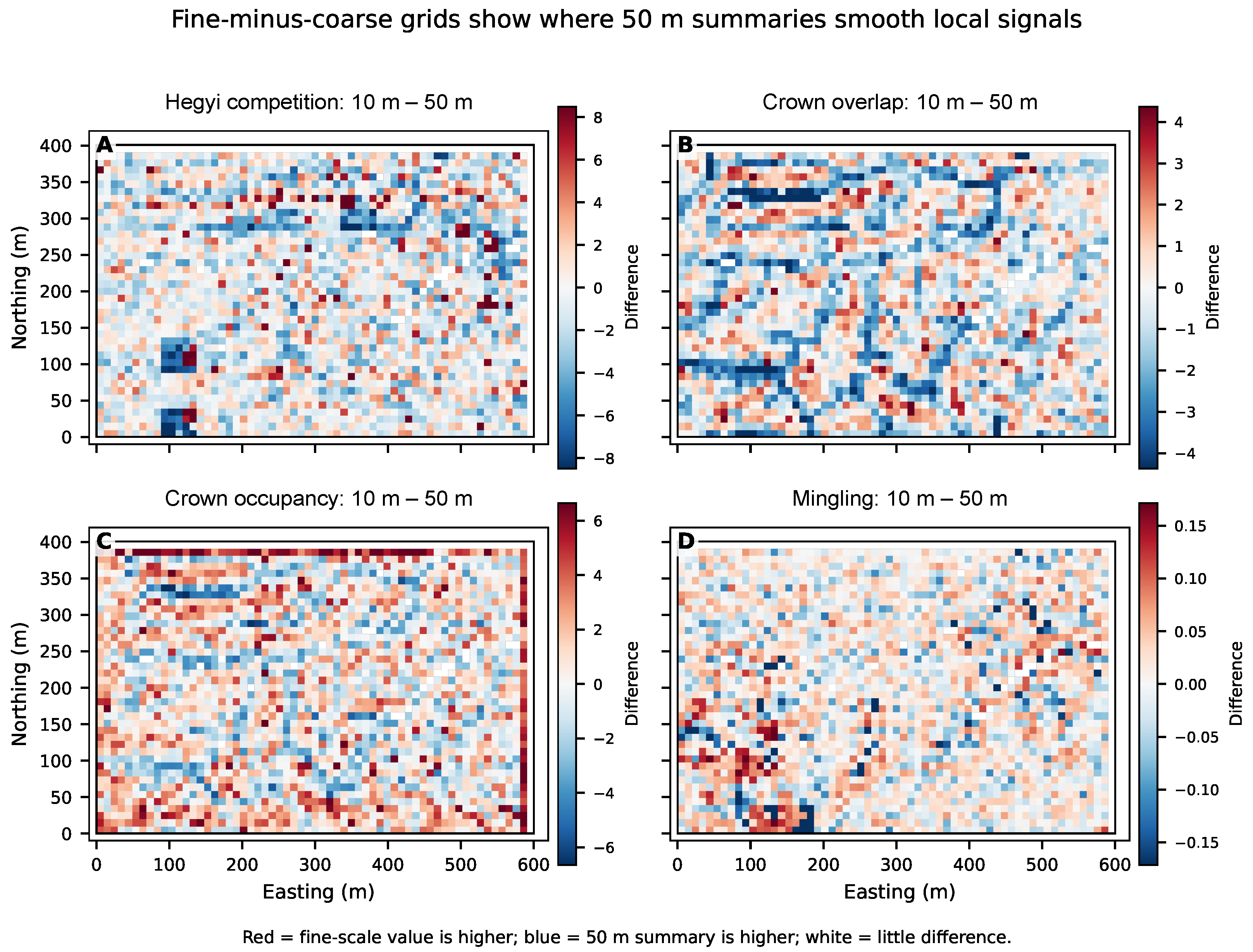
Tree-level indices were aggregated as cell means, except that crown occupancy used summed crown area divided by cell area. For each grain and metric, we calculated the mean, standard deviation, coefficient of variation (CV), median, quartiles, and number of retained cells. Curves at continuous 5 m intervals described whether among-cell variability declined, stabilized, or fluctuated with grain. Fine-minus-coarse difference grids were calculated as each 10 m cell value minus the value of the containing 50 m cell. No scale-sensitivity index or inferential test across nested grains was used.
Because larger cells average more observations, declining CV alone is not evidence of ecological scale structure. We therefore constructed a fixed-pattern random-label benchmark. Tree locations, cell memberships, cell counts, and the marginal distribution of each metric were held constant, while tree-level Hegyi, crown-overlap, mingling, or crown-area values were independently permuted among coordinates. Each of 199 permutations was summarized using the same grids and N ≥ 10 rule, and the observed CV was compared with the permutation median and 2.5–97.5% envelope. This benchmark tested whether high and low metric values were more spatially concentrated than expected after random labeling. It did not simulate a new point pattern or assume complete spatial randomness of the observed locations.

2.8. Point-Pattern and Mark Analyses

To complement fixed-area summaries, we estimated the homogeneous pair-correlation function g ( r ) in 1 m annuli from 0 to 20 m. A reduced-sample border correction retained focal trees only when their distance from the mapped boundary was at least the outer annulus radius. The analysis was repeated for all stems and for stems with DBH ≥ 5 cm. Under a homogeneous Poisson reference, g ( r ) = 1 ; values above or below one indicate excess or deficient pair density at distance r, respectively. We also calculated a normalized DBH mark-correlation function, k m m ( r ) , and the observed probability of conspecific pairs relative to its random-label expectation. Mark summaries used a fixed-seed sample of 20,000 eligible focal trees to control computation while retaining the full neighbor pattern. These diagnostics describe unadjusted spatial pattern and do not account for environmental inhomogeneity.

2.9. Structural Type Classification

Structural types were classified using point-name-derived 20 m inventory units retained after record-level quality control. Candidate features included density, mean DBH, mean height, species richness, Shannon diversity, mingling, neighborhood comparison, Hegyi competition, crown-width distance competition, crown overlap, crown occupancy, basal area per hectare, and large-tree proportion. Features were standardized, projected by PCA, and clustered with K-means. Candidate solutions with 2–7 clusters were evaluated using the silhouette score, Calinski–Harabasz index, Davies–Bouldin index, cluster size, and interpretability of standardized cluster centers. After clustering, types were named based on their dominant standardized attributes. They are within-stand, data-derived groups of inventory units rather than established silvicultural classes.

2.10. Robustness and Sensitivity Analyses

Six sensitivity analyses were conducted. First, all neighborhood, competition, crown-overlap, grid, and hotspot calculations were repeated after restricting both focal trees and candidate neighbors to DBH ≥ 5 cm. This was a complete neighborhood reconstruction, not a post hoc filter of focal-tree outputs. Second, crown width was multiplied by 0.8, 0.9, 1.1, and 1.2, and C O I was recomputed exactly at each multiplier to assess rank and hotspot stability relative to the unperturbed baseline. Third, neighborhood metrics were recalculated using 6 and 8 nearest neighbors. Fourth, the cell threshold was changed from N ≥ 10 to N ≥ 5 and N ≥ 20 . Fifth, point-name-derived 20 m units were compared with coordinate-based 20 m grids using label association and paired-centroid metrics. Sixth, focal trees within 5, 10, and 20 m of the outer boundary were excluded from summaries. Complete results are provided in Supplementary Tables S3–S16 and Figures S6 and S7.

2.11. Statistical Analysis

Associations among Hegyi, crown-width distance competition, and crown overlap were summarized with Spearman rank correlation because the distributions were skewed and relationships were not necessarily linear. Tree-level coefficients were descriptive and were reported without independence-based p-values. To represent spatial uncertainty at an operational grain, we also correlated 20 m cell means and obtained 95% percentile intervals from 2000 spatial-block bootstrap replicates. Cells were grouped into 50 m blocks; blocks, rather than individual trees or cells, were resampled with replacement. Screening maps used 20 m cells, with the top decile defining high Hegyi, high crown overlap, and high crown occupancy and the bottom decile defining low mingling. Analyses were run in Python 3.13.5 with pandas 2.3.1, NumPy 2.4.2, SciPy 1.16.3, scikit-learn 1.8.0, pyproj 3.7.2, and matplotlib 3.10.5 [20,21,22,23,24]. Random procedures used seed 20260802.

3. Results

3.1. Data Characteristics

Cleaning retained 114,524 of 114,731 records (99.82%); 117 records with missing or unrecoverable coordinates and 90 exact duplicate rows were removed. The cleaned inventory contained 297 distinct species labels, compared with 301 before cleaning. DBH, recorded height, and calibrated crown width were all right-skewed, with means of 5.97 cm, 6.09 m, and 3.56 m, respectively (Table 1). The six most abundant taxa accounted for 41.1% of all stems, and no single taxon exceeded 10% (Table 2). Because 66.7% of stems had DBH < 5 cm, the primary neighborhood summaries describe a full inventory containing many small stems rather than canopy-sized trees alone.

3.2. Scale-Response Patterns at 5 m Intervals

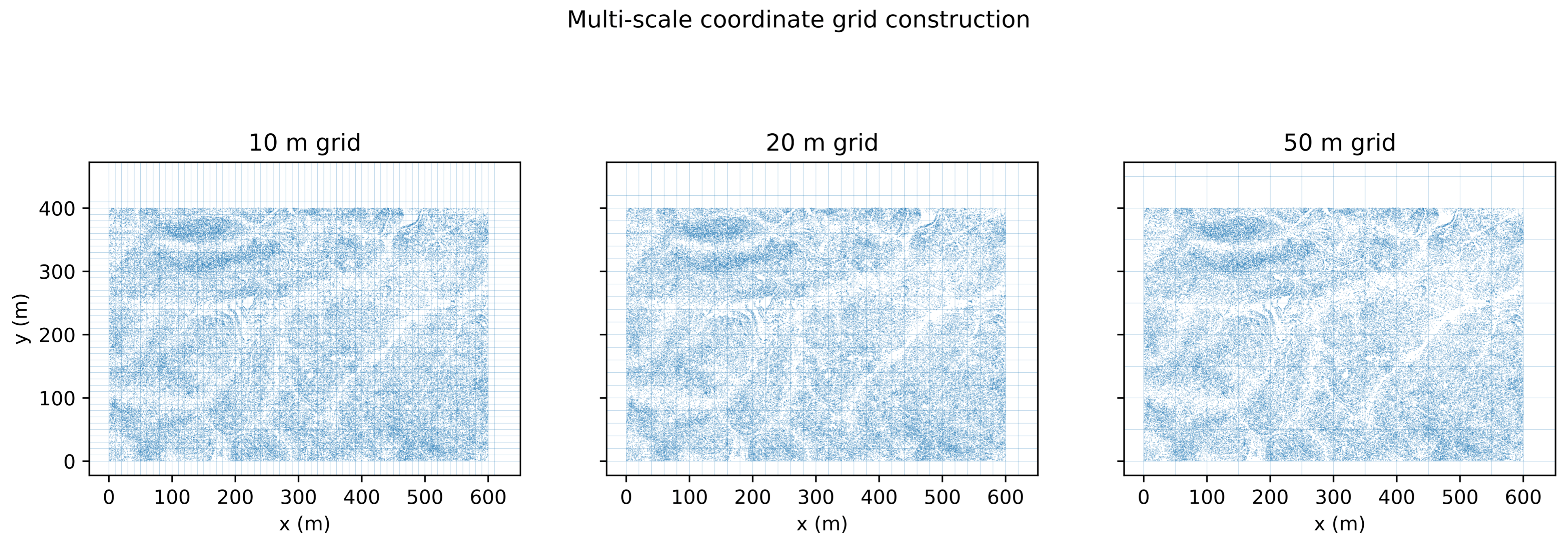
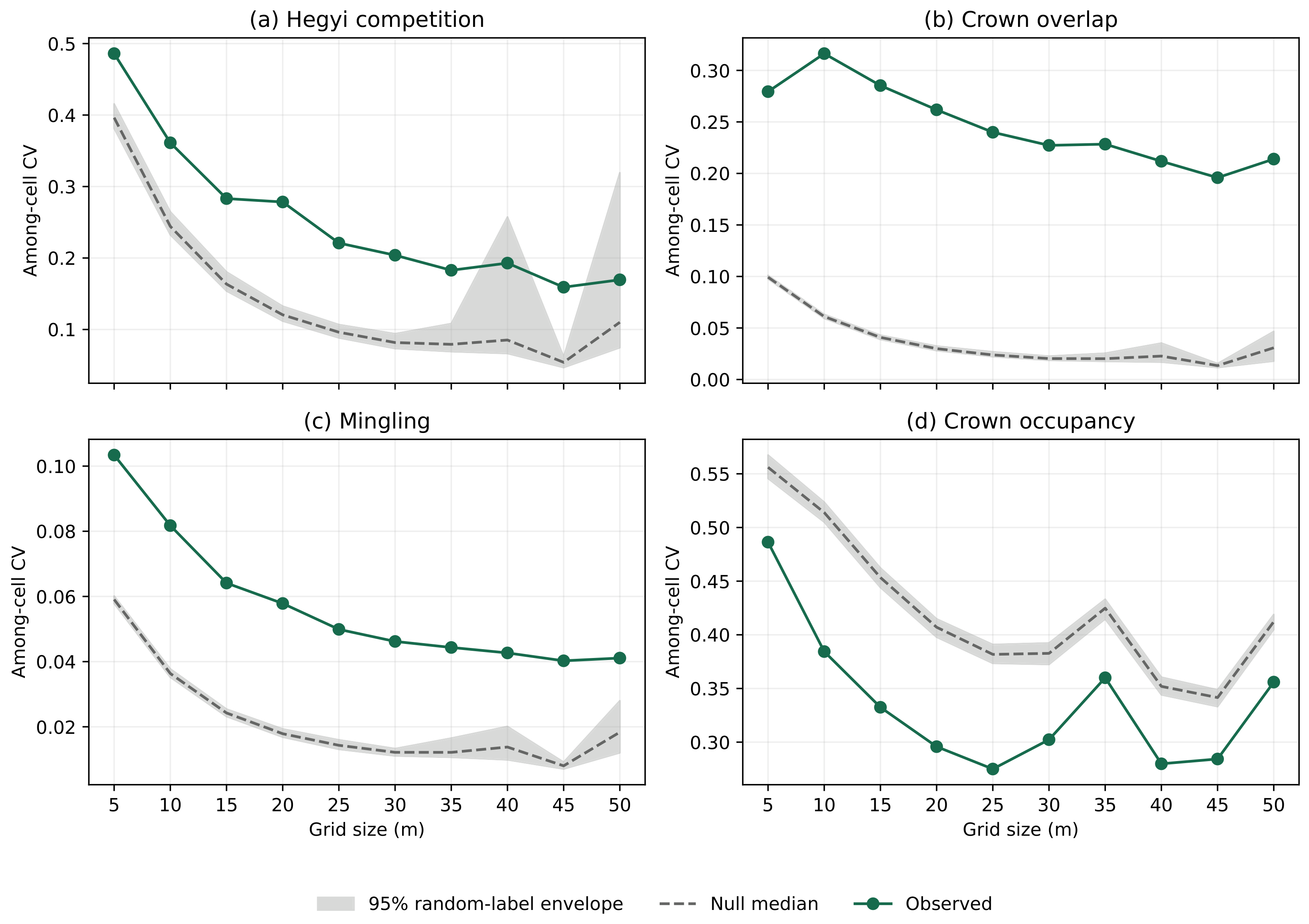
Progressive aggregation of the same mapped trees is shown in Figure 2. Observed CV declined strongly for Hegyi competition and mingling, declined more gradually for crown overlap, and varied non-monotonically for crown occupancy (Figure 3; corresponding cell counts and random-label envelopes are in Supplementary Table S10). The random-label benchmark showed that these changes were not solely an averaging effect. At 20 m, observed CV was 2.31 times the null median for Hegyi (0.278 versus 0.120), 8.73 times for crown overlap (0.262 versus 0.030), and 3.24 times for mingling (0.058 versus 0.018); all exceeded their 95% envelopes. Crown occupancy was below its random-label envelope at every grain, indicating less spatial concentration of crown-area load than expected after assigning crown areas randomly to fixed locations. Hegyi exceeded its envelope from 5 to 35 m and at 45 m, but not at 40 or 50 m, where the null envelope widened sharply. Crown overlap and mingling remained above their envelopes throughout the grain series. Retained-cell counts fell from 5818 at 5 m to 104 at 50 m, so coarse-grain values should not be interpreted as precise stabilization points.

3.3. Fine-to-Coarse Difference Grids and Indicator Maps

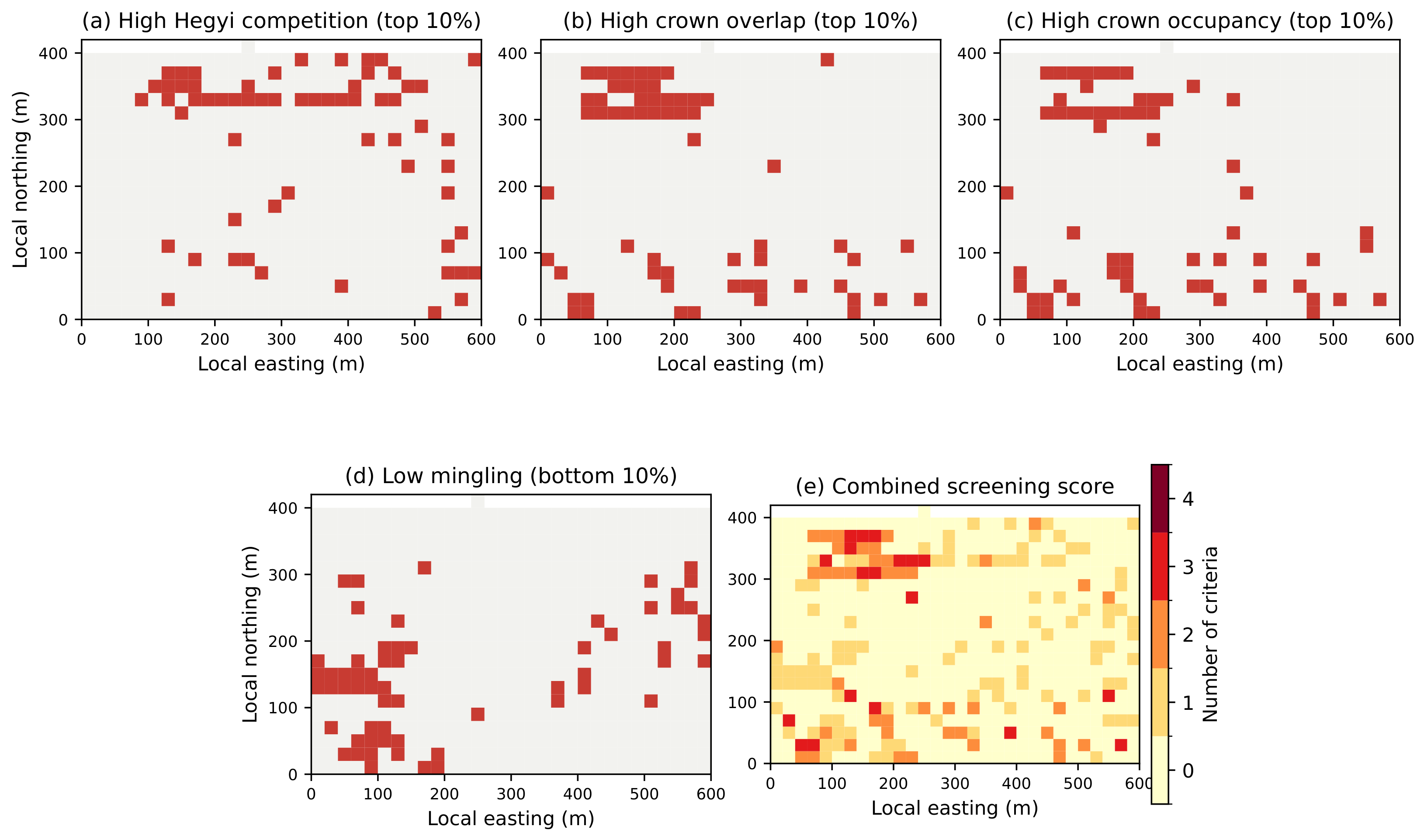
Difference grids showed where 10 m summaries departed from the 50 m unit that contained them (Figure 4). Hegyi competition and crown occupancy had many local positive and negative deviations; mingling differences were smaller but still spatially organized. The 20 m maps flagged high Hegyi, high crown overlap, high crown occupancy, and low mingling, and summed those four flags (Figure 5).

3.4. Associations Between Hegyi and Crown-Competition Metrics

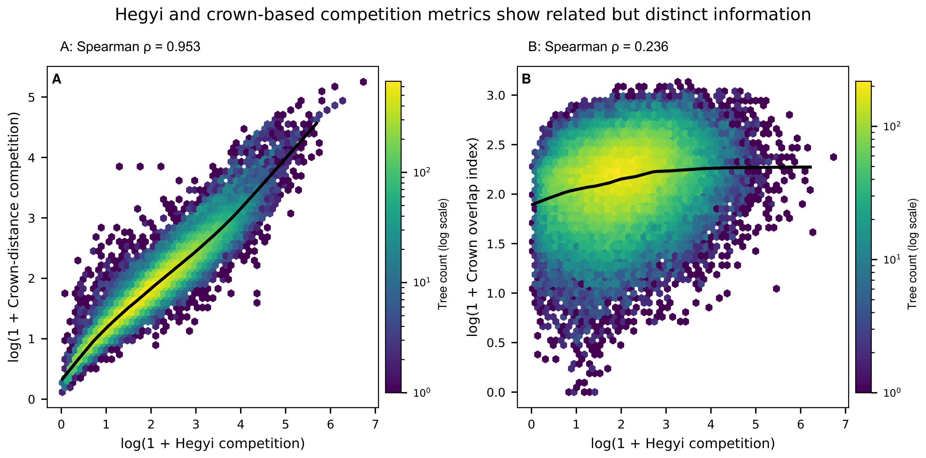
At tree level, Hegyi and crown-width distance competition were strongly associated (Spearman ρ s = 0.953 ), consistent with the power-law DBH–crown model underlying the supplied crown widths. Hegyi was less strongly associated with crown overlap ( ρ s = 0.236 ), and the trend was less linear (Figure 6). At the 20 m cell level, the corresponding coefficients were 0.850 for Hegyi– C C I and 0.390 for Hegyi– C O I ; spatial-block bootstrap 95% intervals were 0.818–0.878 and 0.294–0.484, respectively (Supplementary Table S14). Crown overlap, rather than C C I , was therefore the complementary canopy metric under this crown model.

3.5. Point-Pattern and Mark-Correlation Results

For both stem definitions, the homogeneous pair-correlation function exceeded one throughout 0–20 m (Supplementary Figure S7; Tables S15 and S16). At r = 0.5 m, g ( r ) was 1.308 for all stems and 1.305 for stems with DBH ≥ 5 cm; at r = 19.5 m, the corresponding values were 1.063 and 1.092. Thus, clustering relative to a homogeneous Poisson reference was strongest at short distances but remained detectable at 20 m. The DBH mark correlation was 0.896 at 0.5 m and approached one by 20 m, indicating short-range size segregation rather than clustering of similarly large DBH values. The ratio of observed conspecific pairs to its random-label expectation was 3.49 at 0.5 m and 1.86 at 19.5 m, so same-species association was strong at short range and still present at intermediate range. Environmental inhomogeneity was not modeled.

3.6. Robustness of the Main Patterns

The DBH ≥ 5 cm reanalysis retained 38,128 stems and 227 species. Reconstructing neighborhoods within this subset reduced mean Hegyi from 11.00 to 4.23 and mean crown overlap from 7.85 to 6.09. For the same retained focal stems, rank agreement between all-stem and restricted-neighborhood results remained high for Hegyi ( ρ s = 0.882 ) and C O I ( ρ s = 0.929 ). However, the 20 m top-decile hotspot Jaccard similarity was only 0.222 for Hegyi, compared with 0.658 for crown overlap. The broad decline in Hegyi CV with grain persisted (0.272 at 20 m and 0.130 at 50 m), but local competition priorities were threshold-sensitive.
Other checks supported the main descriptive patterns. Under ± 20 % crown-width perturbations, crown-overlap rank agreement with the exact baseline was ρ s = 0.944 –0.967, and 10 m hotspot Jaccard similarity was 0.831–0.867. Six- and eight-neighbor versions were concordant with the four-neighbor baseline (minimum ρ s = 0.806 ; Hegyi ρ s ≥ 0.950 ). Changing the cell threshold to N ≥ 5 or N ≥ 20 did not reverse the decline in Hegyi CV. Point-name-derived units and coordinate-based 20 m grids were closely aligned (normalized mutual information 0.980). Excluding focal trees within 5 m of the outer boundary changed mean Hegyi by only 0.17% and mean crown overlap by 0.72% (Supplementary Table S3 and Figure S6).

3.7. Structural Types and Management Implications

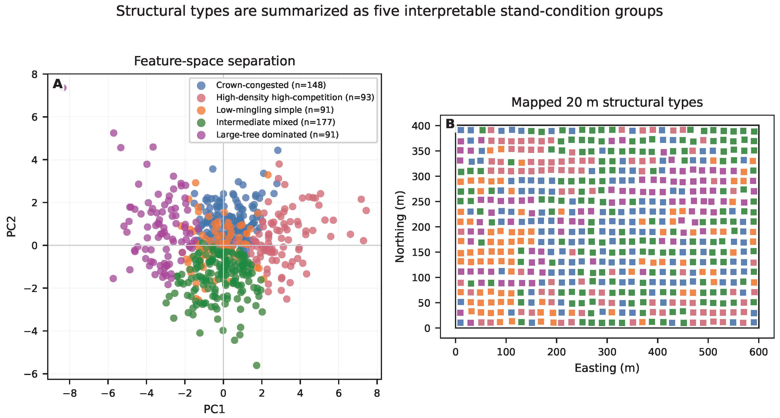
The 600 point-name-derived 20 m inventory units were summarized into five data-driven structural types (Figure 7; Table 4). A candidate cluster combining low mingling with high competition contained only six units and was too small to represent an independent stand-scale type; it was therefore merged with the high-density, high-competition group, while the corresponding local condition remained identifiable in the indicator maps. PCA showed partial separation among groups, which occurred as local patches rather than as a stand-wide mosaic. The high-density, high-competition type had the highest density and relatively high crown overlap, whereas the large-tree-dominated type had lower density and larger mean DBH.

4. Discussion

4.1. Structural Heterogeneity of Subtropical Mixed Forests

The stand was structurally heterogeneous at the inventory scale: species mixing was relatively high, DBH and crown width were right-skewed, and local competition varied markedly. At a broader spatial scope, structural-diversity characteristics have also been reported to differ among mapped plots and ecological zones [25]. Neighborhood variables have been used to describe species-rich mixed stands [2]. In a northern tropical karst rainforest, neighborhood structure calculated for trees with DBH ≥ 5 cm was associated with sapling diversity [26]; that study provides outcome-level context rather than direct evidence about sapling-scale spatial indices. The high mean mingling here indicates that heterospecific nearest neighbors were common. Because the mean uniform-angle index was close to its random expectation, the stand-wide average should not be labeled simply as regular or aggregated. Our hotspot maps and fine-to-coarse difference grids instead show local departures from the stand mean, so management interpretation should retain this within-stand variation.

4.2. Scale Dependence and the Limits of CV-Based Interpretation

Most indicator CVs decreased as grain increased, which is the direction expected when the same trees are placed in larger plots [4,6]. Those studies, together with Fonton et al. on point-pattern summaries and Hou et al. on inventory sampling efficacy, compared alternative sample-plot designs [5,7]. They do not isolate averaging from spatial concentration within one mapped pattern. That isolation is the role of the random-label benchmark used here: after tree positions and indicator marginals are held fixed, Hegyi, C O I , and mingling remained more concentrated than averaging alone would produce, whereas crown occupancy did not. The comparable aggregation study of Maleki et al. changed ALS-derived stand attributes by collapsing pixels into species strata and stands [27]; our summaries instead keep individual stems and change only cell size. At the coarsest grains, especially for Hegyi, permutation envelopes widened and few cells remained, so the results do not support a precise stability threshold.
The point-pattern results reinforced this interpretation across distance: pair density at 0–20 m exceeded the homogeneous-Poisson reference, and same-species association exceeded the random-labeling expectation, consistent with local tree and species aggregation. Because our analysis did not model intensity as a function of terrain, habitat, regeneration history, or management, we treated these departures as exploratory and did not assign them a specific ecological mechanism. For application, 10–20 m grids retained variation useful for local screening, whereas 30–50 m grids provided broader summaries. These are task-dependent reporting grains, not universal ecological optima.

4.3. Complementarity of Hegyi and Crown Metrics

Under the power-law DBH–crown-width model, the strong Hegyi– C C I correlation was expected by construction and remained after spatial summary and block resampling. By contrast, the weak Hegyi– C O I correlation was a result of this dataset, not a result reported by Zambrano et al. Crown-overlap approaches can capture functional-neighborhood effects using crown geometry, although Zambrano et al. used a different crown representation and normalization [9]. UAV-LiDAR studies further show that crown projected area and crown volume can yield competition indices distinct from DBH-based indices [10], and UAV point clouds can retrieve crown width and stand spatial attributes [28]. Terrestrial laser scanning and dendrochronology have also linked measured three-dimensional crown shape to tree-ring variability under neighborhood competition [29]. These studies motivate independently measured crown information but do not validate our study-defined C O I . In the present data, C O I provided the main additional information in the multi-indicator analysis, whereas C C I was more appropriately treated as a sensitivity control. Crown-width perturbation did not change the overall rank pattern, but independent field or LiDAR validation remains necessary.

4.4. Management Implications

Structural classification can support stage-specific diagnosis [30]. At the individual-tree level, Wang et al. proposed prioritizing the removal of trees that were disadvantaged across all four assessed structural dimensions [31]; that proposal does not validate geographic hotspot patches. Here, hotspot maps are descriptive screening outputs derived from our own data. High-density, high-competition units can be checked in the field to determine whether target-tree release is warranted; low-mixing units can prompt assessment of companion-species conservation and regeneration; and canopy-crowded units can warrant crown-space assessment even when stem-based competition is not pronounced. The relatively low agreement between Hegyi hotspots calculated from all stems and from stems with DBH ≥ 5 cm shows that the target layer must be specified before an intervention map is prepared. These maps are screening aids rather than management prescriptions.

4.5. Limitations and Future Work

Several limitations constrain interpretation. The inventory was cross-sectional and therefore cannot establish causal effects on growth, mortality, diversity, or management response. Crown width was calibrated or estimated and is subject to allometric and image-extraction error. Boundary truncation can omit true neighbors and bias neighborhood indices [13]; in our own 5 m outer-buffer check, mean Hegyi and C O I changed by 0.17% and 0.72%, respectively (Supplementary Table S3). In our implementation, the random-labeling test held observed locations fixed and permuted indicator or species marks; it was not a test of complete spatial randomness. Separately, unmarked g ( r ) was assessed against a homogeneous Poisson reference. Neither analysis corrected habitat-driven intensity gradients. Local Hegyi priority areas were sensitive to whether small stems were included. Abnormal tree-height records and missing survey metadata further limit interpretation. Unit screening and the small number of cells at coarse grains also affect uncertainty estimates, and transferability to other stands remains untested. Future work should combine repeated inventories with independent crown measurements. UAV point clouds provide one route for retrieving crown width and stand attributes [28]. UAV LiDAR can provide crown-projected-area and crown-volume metrics derived directly from point clouds rather than from DBH allometry [10], while terrestrial laser scanning can characterize three-dimensional crown shape [29]. Environmental covariates should also be incorporated into inhomogeneous and predictive models.

5. Conclusions

Mapped individual-tree data showed grain-dependent patterns of stand structure and competition. Fixed-pattern random labeling indicated that Hegyi, crown overlap, and mingling retained spatial contrast beyond arithmetic averaging at most grains, while pair and mark correlations documented short-range clustering and conspecific association. Coarse-grain estimates were less certain because few cells remained. Under the available crown model, C C I largely tracked Hegyi, whereas crown overlap provided the main complementary canopy-crowding signal. The DBH ≥ 5 cm reanalysis preserved broad rank and scale patterns but substantially changed local Hegyi hotspot membership, making stem-size definition essential for management screening. Accordingly, 10–20 m and 30–50 m units are best treated as task-dependent local and broader reporting grains rather than universal optima.

Supplementary Materials

The following supporting information can be downloaded at https://www.mdpi.com/article/10.3390/f17091124/s1: Figures S1–S5, variable distributions, dominant species, and data screening; Figure S6, robustness and sensitivity analyses; Figure S7, pair- and mark-correlation functions; Tables S1 and S2, species labels and dominant taxa; Tables S3–S8, crown-width, neighbor-number, cell-threshold, inventory-unit, and boundary tests; Table S9, continuous scale-response statistics; Table S10, random-label CV benchmark; Tables S11 and S12, DBH-threshold summaries and agreement; Table S13, summary of complete grid scales under two DBH thresholds; Table S14, spatial-block correlations; Tables S15 and S16, pair- and mark-correlation values.

Author Contributions

Conceptualization, B.S. and J.L.; methodology, B.S.; software, B.S.; validation, B.S. and Y.Z.; formal analysis, B.S.; investigation, B.S. and Y.Z.; resources, J.L.; data curation, B.S. and Y.Z.; writing—original draft preparation, B.S.; writing—review and editing, J.L. and Y.Z.; visualization, B.S.; supervision, J.L.; project administration, J.L. All authors have read and agreed to the published version of the manuscript.

Funding

This research received no external funding.

Institutional Review Board Statement

Not applicable.

Informed Consent Statement

Not applicable.

Data Availability Statement

The individual-tree inventory is governed by a cooperation agreement with Nanshan Nature Reserve. Owing to institutional and data-use restrictions, the study data are available from the corresponding author upon reasonable request. Processed summary tables and figures are included with the submission; analysis scripts may also be requested from the corresponding author, subject to the same institutional data-use restrictions.

Acknowledgments

We thank the management of Nanshan Nature Reserve for supporting access to the field-inventory data and the field team members who participated in individual-tree measurements. We also thank the School of Computer Science and Mathematics, Central South University of Forestry and Technology, for providing computational support during manuscript preparation.

Conflicts of Interest

The authors declare no conflicts of interest.

References

  1. Pommerening, A. Approaches to quantifying forest structures. Forestry 2002, 75, 305–324. [Google Scholar] [CrossRef] [Scilit]
  2. Aguirre, O.; Hui, G.; von Gadow, K.; Jiménez, J. An analysis of spatial forest structure using neighbourhood-based variables. For. Ecol. Manag. 2003, 183, 137–145. [Google Scholar] [CrossRef] [Scilit]
  3. Hegyi, F. A simulation model for managing jack-pine stands. In Growth Models for Tree and Stand Simulation: Proceedings of Meetings in 1973; Fries, J., Ed.; Number 30 in Research Notes; Department of Forest Yield Research, Royal College of Forestry: Stockholm, Sweden, 1974; pp. 74–90. [Google Scholar]
  4. Maleki, K.; Kiviste, A. Effect of sample plot size and shape on estimates of structural indices: A case study in mature silver birch (Betula pendula Roth) dominating stand in Järvselja. For. Stud. 2015, 63, 130–150. [Google Scholar] [CrossRef] [Scilit]
  5. Fonton, N.H.; Atindogbe, G.; Hounkonnou, N.M.; Dohou, R.O. Plot size for modelling the spatial structure of Sudanian woodland trees. Ann. For. Sci. 2011, 68, 1315–1321. [Google Scholar] [CrossRef] [Scilit]
  6. Lombardi, F.; Marchetti, M.; Corona, P.; Merlini, P.; Chirici, G.; Tognetti, R.; Burrascano, S.; Alivernini, A.; Puletti, N. Quantifying the effect of sampling plot size on the estimation of structural indicators in old-growth forest stands. For. Ecol. Manag. 2015, 346, 89–97. [Google Scholar] [CrossRef] [Scilit]
  7. Hou, Z.; Xu, Q.; Hartikainen, S.; Antilla, P.; Packalen, T.; Maltamo, M.; Tokola, T. Impact of plot size and spatial pattern of forest attributes on sampling efficacy. For. Sci. 2015, 61, 847–860. [Google Scholar] [CrossRef] [Scilit]
  8. Niklas, K.J. Plant Allometry: The Scaling of Form and Process; University of Chicago Press: Chicago, IL, USA, 1994. [Google Scholar]
  9. Zambrano, J.; Fagan, W.F.; Worthy, S.J.; Thompson, J.; Uriarte, M.; Zimmerman, J.K.; Umaña, M.N.; Swenson, N.G. Tree crown overlap improves predictions of the functional neighbourhood effects on tree survival and growth. J. Ecol. 2019, 107, 887–900. [Google Scholar] [CrossRef] [Scilit]
  10. Puletti, N.; Guasti, M.; Innocenti, S.; Cesaretti, L.; Chiavetta, U. A semi-automatic approach for tree crown competition indices assessment from UAV LiDAR. Remote Sens. 2024, 16, 2576. [Google Scholar] [CrossRef] [Scilit]
  11. Stoyan, D.; Penttinen, A. Recent applications of point process methods in forestry statistics. Stat. Sci. 2000, 15, 61–78. [Google Scholar] [CrossRef] [Scilit]
  12. Pang, L.; Xie, D.; Sharma, R.P.; Xu, D.; Fu, L. Developing GIS-based algorithm of stand spatial structure index and its implementation. Forests 2024, 15, 1755. [Google Scholar] [CrossRef] [Scilit]
  13. Pommerening, A.; Stoyan, D. Edge-correction needs in estimating indices of spatial forest structure. Can. J. For. Res. 2006, 36, 1723–1739. [Google Scholar] [CrossRef] [Scilit]
  14. Shannon, C.E. A mathematical theory of communication. Bell Syst. Tech. J. 1948, 27, 379–423. [Google Scholar] [CrossRef] [Scilit]
  15. Simpson, E.H. Measurement of diversity. Nature 1949, 163, 688. [Google Scholar] [CrossRef] [Scilit]
  16. Pielou, E.C. Species-diversity and pattern-diversity in the study of ecological succession. J. Theor. Biol. 1966, 10, 370–383. [Google Scholar] [CrossRef] [Scilit]
  17. von Gadow, K.; Hui, G.; Albert, M. Das Winkelmaß—Ein Strukturparameter zur Beschreibung der Individualverteilung in Waldbeständen. Cent. Fur Gesamte Forstwes. 1998, 115, 1–10. [Google Scholar]
  18. Li, Y.; Hui, G.; Zhao, Z.; Hu, Y. The bivariate distribution characteristics of spatial structure in natural Korean pine broad-leaved forest. J. Veg. Sci. 2012, 23, 1180–1190. [Google Scholar] [CrossRef] [Scilit]
  19. Hui, G.; von Gadow, K. Das Winkelmaß: Herleitung des optimalen Standardwinkels. Allg. Forst Jagdztg. 2002, 173, 173–177. [Google Scholar]
  20. McKinney, W. Data Structures for Statistical Computing in Python. In Proceedings of the 9th Python in Science Conference; van der Walt, S., Millman, J., Eds.; SciPy: Austin, TX, USA, 2010; pp. 56–61. [Google Scholar] [CrossRef] [Scilit]
  21. Harris, C.R.; Millman, K.J.; van der Walt, S.J.; Gommers, R.; Virtanen, P.; Cournapeau, D.; Wieser, E.; Taylor, J.; Berg, S.; Smith, N.J.; et al. Array programming with NumPy. Nature 2020, 585, 357–362. [Google Scholar] [CrossRef] [Scilit]
  22. Virtanen, P.; Gommers, R.; Oliphant, T.E.; Haberland, M.; Reddy, T.; Cournapeau, D.; Burovski, E.; Peterson, P.; Weckesser, W.; Bright, J.; et al. SciPy 1.0: Fundamental algorithms for scientific computing in Python. Nat. Methods 2020, 17, 261–272, Correction in Nat. Methods 2020, 17, 352. [Google Scholar] [CrossRef] [Scilit]
  23. Pedregosa, F.; Varoquaux, G.; Gramfort, A.; Michel, V.; Thirion, B.; Grisel, O.; Blondel, M.; Prettenhofer, P.; Weiss, R.; Dubourg, V.; et al. Scikit-learn: Machine Learning in Python. J. Mach. Learn. Res. 2011, 12, 2825–2830. [Google Scholar]
  24. Hunter, J.D. Matplotlib: A 2D Graphics Environment. Comput. Sci. Eng. 2007, 9, 90–95. [Google Scholar] [CrossRef] [Scilit]
  25. Dong, L.; Bettinger, P.; Liu, Z. Stand spatial structural diversity: Developing and validating a novel index. For. Ecol. Manag. 2024, 569, 122157. [Google Scholar] [CrossRef] [Scilit]
  26. Li, L.; Ma, R.; Wang, B.; Huang, F.; Li, J.; Lu, F.; Xiang, W.; Li, D.; Li, X.; Guo, Y. Stand spatial structure promotes tree growth and sapling diversity in northern tropical karst seasonal rainforest. Front. Plant Sci. 2025, 16, 1649999. [Google Scholar] [CrossRef] [Scilit]
  27. Maleki, K.; Astrup, R.; Cattaneo, N.; Lara Henao, W.; Antón-Fernández, C. The effects of data aggregation on long-term projections of forest stands development. For. Ecosyst. 2024, 11, 100199. [Google Scholar] [CrossRef] [Scilit]
  28. Huang, X.; Chen, Y.; Tan, H.; Zhang, Y.; Yu, S.; Chen, X.; Yu, K.; Liu, J. Extraction of the spatial structure of Chinese fir plantations stands based on unmanned aerial vehicle and its effect on AGB. For. Ecol. Manag. 2024, 558, 121800. [Google Scholar] [CrossRef] [Scilit]
  29. Ahmed, S.; Hilmers, T.; Uhl, E.; Jacobs, M.; Bohnhorst, L.; Kolisnyk, B.; del Río, M.; Pretzsch, H. Neighborhood competition modulates the link between crown structure and tree ring variability in monospecific and mixed forest stands. For. Ecol. Manag. 2024, 560, 121839. [Google Scholar] [CrossRef] [Scilit]
  30. Sheng, Q.; Dong, L.; Liu, Z. Optimizing stand spatial structure at different development stages in mixed hard broadleaf forests. Forests 2024, 15, 1653. [Google Scholar] [CrossRef] [Scilit]
  31. Wang, Z.; Li, Y.; Wang, G.; Zhang, Z.; Chen, Y.; Liu, X.; Peng, R. Drivers of spatial structure in thinned forests. For. Ecosyst. 2024, 11, 100182. [Google Scholar] [CrossRef] [Scilit]
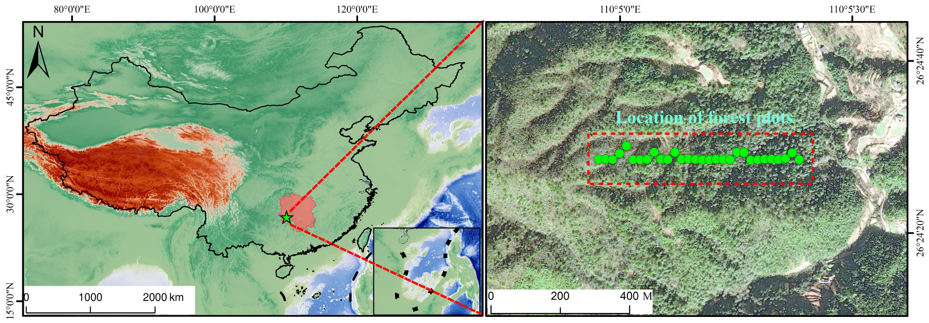
Figure 1. Study area and forest-plot transect in Nanshan Nature Reserve, Suining County, Hunan Province, China. (Left): National-scale location map highlighting Hunan Province. Pink represents Hunan Province; a green star indicates the research area; the color of the background map indicates the terrain and waters. (Right): Forest-plot location on satellite imagery; the green marker denotes the plot and the red dashed rectangle denotes the surveyed transect. Coordinates are WGS84, with a reference point near 110.086° E, 26.408° N. Basemap source: Esri World Imagery (Esri, Maxar, Earthstar Geographics); map prepared by the authors.
Forests 17 01124 g001
Figure 2. The same mapped trees summarized in progressively coarser spatial units. A representative 120 m × 120 m area is shown for 10, 20, and 50 m grids to make scale aggregation explicit.
Forests 17 01124 g002
Figure 3. Observed and random-label scale-response curves at 5 m intervals. The vertical axis is the coefficient of variation among retained grid cells ( N ≥ 10 trees). The solid green line is the observed value; the dashed gray line and shaded band are the median and 95% envelope from 199 fixed-pattern random-label permutations. The benchmark retains tree locations, cell counts, and the marginal distribution of each metric.
Forests 17 01124 g003
Figure 4. Fine-minus-coarse difference grids. (A) Hegyi competition; (B) crown overlap; (C) crown occupancy; (D) mingling. Each 10 m cell is compared with the containing 50 m cell. Red indicates a higher fine-grain value, blue indicates the opposite, and near-white cells indicate little difference.
Forests 17 01124 g004
Figure 5. Integrated 20 m indicator maps. Panels (a–d) flag retained cells in the top decile of Hegyi competition, crown overlap, or crown occupancy, or the bottom decile of mingling; panel (e) sums the four binary criteria. Axes are local projected metres, labeled every 100 m from 0–600 m easting and 0–400 m northing.
Forests 17 01124 g005
Figure 6. Relationships between Hegyi competition and the two crown-competition metrics. (A) Crown-width distance competition ( C C I ); (B) Crown Overlap ( C O I ). Hexagonal bins summarize dense tree-level point clouds, and black LOWESS curves show nonlinear trends. Spearman correlations use all trees. Axes are log-transformed to improve visibility in dense regions.
Forests 17 01124 g006
Figure 7. Structural-type classification in multivariate feature space and across mapped inventory units. Panel (A) shows PCA scores for five interpretable data-driven groups; Panel (B) shows their spatial distribution. Local low-mingling/high-competition units are treated as priority screening units rather than an additional stand-scale type.
Forests 17 01124 g007
Table 1. Study-site, inventory-design, and data-quality summary. The census threshold was DBH ≥ 1.0 cm. Unit-level and taxon-level sampling statistics are in Table 2.
ItemValue
LocationNanshan Nature Reserve, Hunan, China (26°24′22″–26°24′35″ N; 110°04′59″–110°05′21″ E)
Forest typeSubtropical evergreen broad-leaved secondary forest
ElevationApproximately 800–1200 m a.s.l.
Mapped coordinate extent600.4 m × 400.8 m (approximately 24 ha)
Encoded inventory design30 plot groups comprising 600 20 m × 20 m inventory units
Original records114,731
Final records for analysis114,524 (99.82%)
Distinct recorded species labels297
Missing or unrecoverable coordinates117 (0.10%)
Coordinates recovered from DMS/raw strings52 (0.05%)
Exact duplicate records removed90 (0.08%)
Reported heights below 1.3 m, flagged328 (0.29% of final records)
DBH (cm), mean ± SD (range) 5.97 ± 7.99 (1.00–121.30)
Reported tree height (m), mean ± SD (range) 6.09 ± 5.45 (0.50–70.00)
Calibrated crown width (m), mean ± SD (range) 3.56 ± 2.42 (0.60–24.75)
Stems with DBH < 5 cm (of final records)66.7%
Table 2. Sampling-site statistics for the single subtropical evergreen broad-leaved stand. Upper block: Unweighted summaries of the 600 encoded 20 m inventory units. Lower block: Stem-weighted summaries by recorded taxon, including planted/associated Cunninghamia lanceolata.
600 Inventory Units (One Forest Type)Mean ± SDMinMax
Stems per unit 190.87 ± 73.73 25472
Recorded taxa per unit 35.63 ± 7.13 1167
Unit-mean DBH (cm) 6.27 ± 1.32 2.6416.57
Unit-mean height (m) 6.21 ± 1.17 3.6611.92
Recorded TaxonStems ( n )Inventory (%)Mean DBH (cm), Height (m)
Castanopsis fargesii11,1439.736.30, 5.92
Castanopsis tibetana79736.965.22, 4.52
Rhododendron latoucheae76276.664.05, 3.94
Lindera pulcherrima var. hemsleyana75686.613.03, 4.43
Camellia oleifera65175.692.68, 3.46
Dendropanax dentiger62085.424.62, 5.22
Cunninghamia lanceolata34032.9710.49, 8.49
Other recorded taxa (290 labels)64,08555.966.82, 6.99
Table 3. Definitions, calculation basis, and interpretation of the main structural and competition indices used in this study.
IndexCalculation BasisInterpretation in This Study
Mingling index ( M i )Tree level, four nearest neighbors; unit means of tree-level values M i = 1 4 ∑ j = 1 4 v i j , where v i j = 1 if neighbor j differs in species from target i and 0 otherwise. Higher values indicate stronger local species mixing.
Neighborhood comparison ( U i )Tree level, four nearest neighbors; unit means U i = 1 4 ∑ j = 1 4 k i j , where k i j = 1 if neighbor j has larger DBH than target i. Higher values indicate a local size disadvantage of the target tree.
Uniform angle index ( W i )Tree level, four nearest neighbors; unit meansAngular arrangement of the four neighbors using the simulation-derived 72 ° standard angle [19]. Values near 0.5 indicate a near-random local horizontal pattern; lower/higher values indicate more regular/clumped arrangements.
Hegyi competition ( C I i )Tree level, four nearest neighbors C I i = ∑ j = 1 4 D B H j / D B H i d i j . Classical distance-dependent competition based on stem-size ratios [3].
Crown-width distance competition ( C C I i )Tree level, four nearest neighbors C C I i = ∑ j = 1 4 C W j / C W i d i j . Formally analogous to Hegyi but uses calibrated crown width. Because C W was derived from a power-law DBH–crown model, C C I largely tracks Hegyi and is not treated as independent evidence of complementarity.
Crown-overlap index ( C O I i )Tree level; radius search on circular crownsRelative two-circle crown-overlap load on the target crown; can exceed 1 when several neighbors overlap the same target. Provides the main crown-geometry signal complementary to Hegyi.
Crown-occupancy ratioSpatial unit (grid cell or inventory unit)Summed circular crown area divided by unit area; a crown-space load indicator rather than a literal canopy-cover fraction.
Basal areaTree level; summed or standardized to unitsStem cross-sectional area describing local stocking.
Shannon diversity ( H ′ )Spatial unit, species counts of stems in the unitCombined species richness and evenness within the spatial unit [14].
Table 4. Structural types derived by K-means clustering of standardized attributes of point-name-based 20 m inventory units. A six-unit rare low-mingling/high-competition cluster was merged into the high-density high-competition group; local hotspots are mapped separately in Figure 5.
Structural TypeN UnitsMain Diagnostic SignalManagement-Oriented Interpretation
Crown-congested type148High crown overlap and high crown occupancy despite moderate density.Reduce local crown-space pressure while retaining mixture; target-tree crown release and removal of suppressed or poorly formed competitors could be considered.
High-density high-competition type93Highest density, highest Hegyi competition, and high crown-overlap load.Screen for local competition reduction; selective thinning around target trees could be considered while retaining healthy large trees and valuable species.
Low-mingling structurally simple type91Lowest mingling and lower species richness relative to other types.Maintain companion species and regeneration diversity; retain rare or companion species and avoid reinforcing single-species dominance.
Intermediate mixed-structure type177Moderate competition and relatively balanced structural attributes.Maintain current structure and monitor local deviations; low-intensity, site-specific tending is most appropriate where local hotspots are present.
Large-tree dominated type91Lowest density, highest mean DBH, and weaker local competition.Protect healthy dominant trees while supporting recruitment; microsite improvement for suppressed recruits could be considered where regeneration is limited.
Disclaimer/Publisher’s Note: The statements, opinions and data contained in all publications are solely those of the individual author(s) and contributor(s) and not of MDPI and/or the editor(s). MDPI and/or the editor(s) disclaim responsibility for any injury to people or property resulting from any ideas, methods, instructions or products referred to in the content.