Simulating the Sawing of Beech (Fagus grandifolia) and Birch (Betula papyrifa) Logs

Abstract

One of the most important metrics for analyzing hardwood sawmill performance with respect to profitability is knowing the expected yield from any specific log. The Log Recovery Analysis Tool (LORCAT) is a spreadsheet-based sawmill simulation and analysis tool that was developed to provide this information. As such, LORCAT depends on recorded grade recovery data to determine the quality and volume using the NHLA grade of the sawn lumber. Recently, the grade recovery data of LORCAT was expanded to include beech (Fagus grandifolia) and paper birch (Betula papyrifa), allowing the software to simulate sawing and analysis of these species. While the data are based on North American species, grading systems, and economic assumptions, with differences in species, silvicultural, logging (bucking), and sawing practices acknowledged, LORCAT can be used to emulate the sawing of European logs. Overall, LORCAT can simulate and analyze the sawing of 13 common North American hardwood species (red oak, white oak, black oak, scarlet oak, chestnut oak, red maple, sugar maple, yellow poplar, American beech, paper birch, yellow birch, black cherry, and basswood) for small-end diameters ranging from 20 cm to 90 cm, and report the volume and the quality of lumber produced, as well as the volume and weight of residual products.

1. Introduction

The recovery of lumber and other byproducts in hardwood sawmills is influenced by numerous factors. This includes log characteristics, such as species, diameter, length, taper, and grade, as well as sawing parameters, such as kerf size, sawing variation, and the types or products being sawn [1]. Understanding and examining these relationships among these interdependent factors helps operators to maximize yield and profit.

The Log Recovery Analysis Tool (LORCAT) software [2] was built on common spreadsheet software (Microsoft Excel^® 16.109.2 (The use of trade, firm, or corporation names in this publication is for the information and convenience of the reader. Such use does not constitute an official endorsement or approval by Virginia Tech or the U.S. Department of Agriculture or the Forest Service of any product or service to the exclusion of others that may be suitable.)) or LibreOffice^® 26.2.3.2 to analyze factors and interactions to optimize mill profitability. Unlike past software [3,4,5,6], which required extensive data and specialized training, LORCAT avoids these complexities by requiring minimal setup and yields easily understood results. Similar tools exist in Europe, such as CutLog [7]. However, LORCAT is a free software, and its source code can be accessed and altered under 17 U.S.C. §105 [8]. LORCAT can analyze a single log or up to 1000 logs with different log dimensions and log quality classes, and can return yields, quantity of product, and residuals, as well as costs, profitability, and the expected time to finish a job. 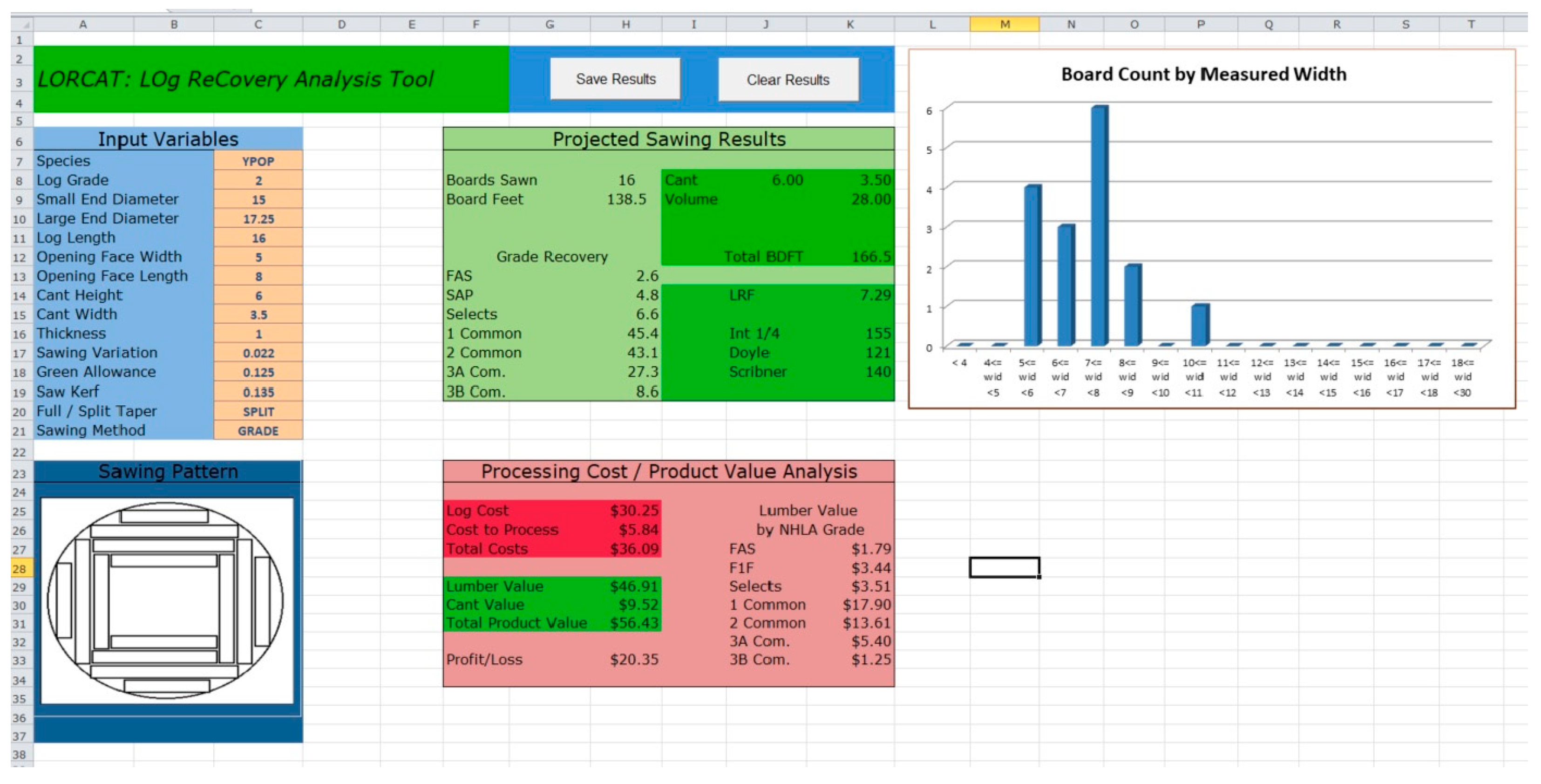Figure 1 shows the main user interface where all the input variables, projected sawing results, and processing cost/product value analyses are displayed.

The input variables (Figure 1) allow users to simulate most of the possible scenarios encountered in their mill, as well as to simulate the sawing of logs ranging from a 200 to 889 mm small-end diameter (SED) and lengths of 2.4 to 4.9 m with a variety of sawing options. The projected sawing results demonstrate sawing a log into boards, including cant size, board-foot volumes by NHLA class [9], and board-foot volumes by International ¼, Doyle, and Scribner log scales [10]. Processing cost/product value analyses offer information on the costs incurred and the value recovered from the log sawn.

While geometric calculations report the yield from sawing a specific log, predicting the volume of dried lumber in each NHLA quality class requires information about the grade [11] of the log being sawn and the probability of the resulting distribution of NHLA quality classes in the lumber [12]. LORCAT uses the hardwood log-grade recovery tables that were created from measuring and recording the sawing of thousands of hardwood logs at 40 mills in 18 states [13]. These tables contain recovery information for 18 species, categorized by SED and USDA FS factory log grades [11]. However, Thomas and Brown [14] raised several issues with the log recovery tables by Hanks et al. [12], highlighting their limited application. According to Thomas and Brown [14], the number of samples recorded for some species, log grades, SEDs, and log length combinations can be small (as few as a single log in some cases), preventing accurate averages. Secondly, the results recorded in the Hanks et al. 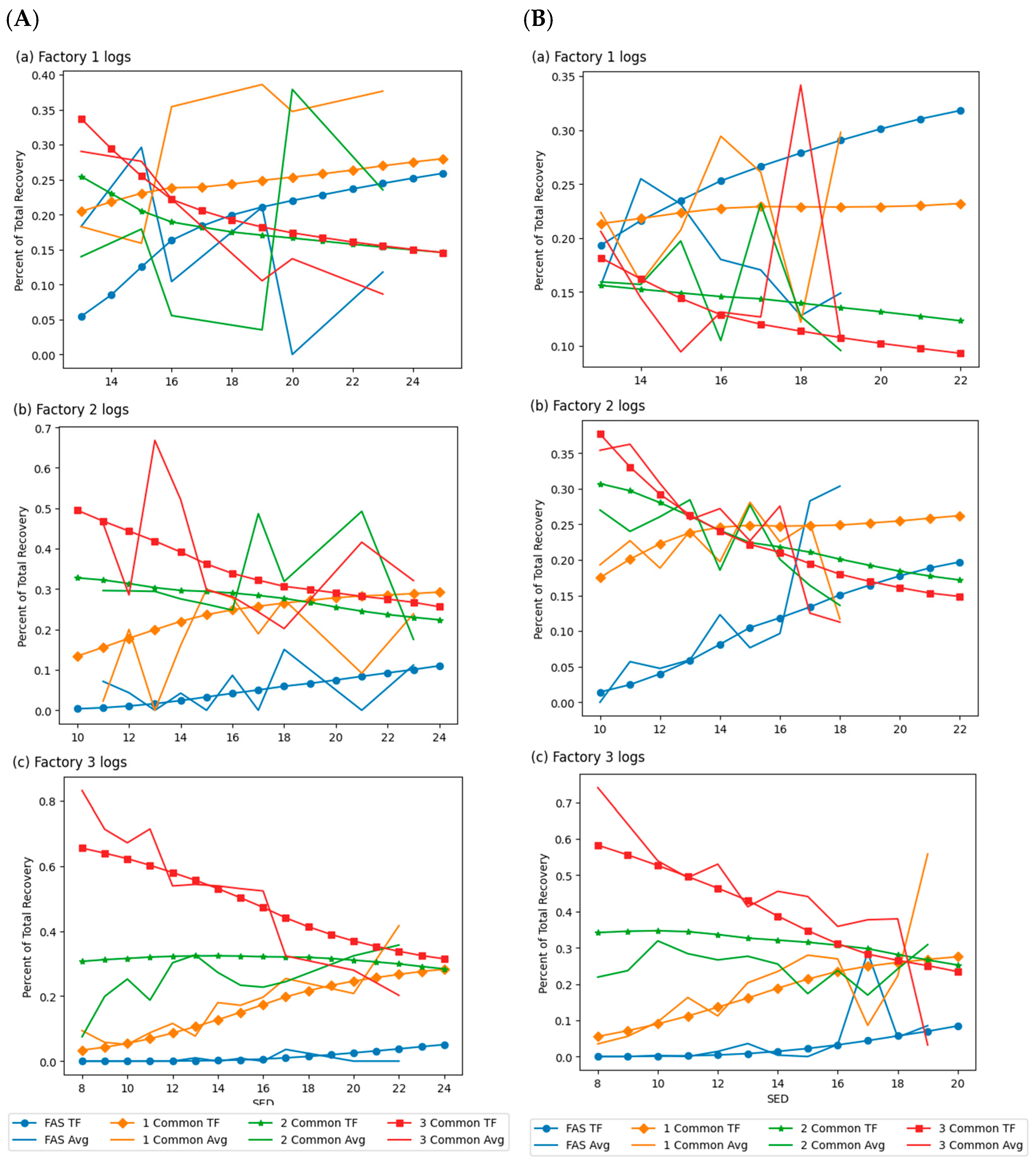tables [12] are sometimes erratic, with notable differences between similar SEDs, as shown in Figure 2 for beech (A) and birch (B), respectively.

Thomas and Brown [13] undertook efforts to eliminate the erratic nature of the Hanks et al. tables [11] so that the NHLA recovery rates [9] by USDA factory log grade [10], species, and SED were more consistent. However, they reported that using regression models to reliably predict grade recovery was not successful because of the non-parametric nature of the data and the requirement that the sum of grade recovery percentages must be 100 percent. Therefore, artificial neural networks were employed to create a predictive model from the log-grade recovery tables [12] for NHLA lumber-grade recovery [9] from USDA FS factory log-graded logs [11].

Neural networks emulate biological neural systems by using mathematical formulas [15] and a series of interconnected elements called neurons. Neurons independently process numeric information and pass it on to the next neuron with an associated weight, emphasizing or de-emphasizing the signal [16]. Deep learning neural network models are typically comprised of hundreds or thousands of such neurons. Furthermore, neural networks excel at modeling complex, nonlinear, parametric, and non-parametric problems. To model the log-grade recovery problem based on Hanks et al.’s [12] data, TensorFlow 2.21 [17], an open-source library for deep learning neural networks, was used.

2. Methods

To model the log-grade recovery for beech and birch, the authors followed the methods explained in Thomas et al. [18]. As neural networks benefit from having a large training dataset, the Wood et al. [13] dataset was used. This dataset offered the largest number of logs across all species after removing logs that were not graded to USFS Factory log grades [11].

Table 1. Number of logs available in Wood et al. for training and validating the neural network.

Number of Logs
USFS Log Grade
Total	Factory 3	Factory 2	Factory 1	Species
424	231	154	39	Birch
101	64	30	7	Beech
10,857	4718	4039	2100	Other Species 1
11,382	5013	4223	2146	Total

¹ Quercus: rubra, alba, velutina, coccinea, macrocarpa, lyrata, falcata, and montana; Acer: rubrum, saccharum, and saccharinum; Ulmus americana; Fraxinus sp.; Populus: tremuloides, grandidentata, and balsamifera; Liriodendron tulipifera; Betula: papyrifera, alleghaniensis, and neoalaskana; Carya sp.; Prunus serotina; Tilia americana; Fagus grandifolia; Magnolia acuminata.

shows the logs available for all species, as well as for birch and beech, for Factory 1, 2, and 3 graded logs, respectively.

The species, log grade, scaling diameter (small-end diameter inside the bark), and scaling deduction indicator, recorded by Hanks et al. [12], were used as input into the deep learning neural network created using the TensorFlow [17], Keras [19], and SciKit-Learn development libraries [20]. The deduction indicator was introduced by Hanks et al. [12] to take into account logs with sweep, crook, or a defect that was significant to a degree that it reduced recovery. Data for 25 hardwood species (Table 1) and three log grades (Factories 1, 2, and 3) were encoded into 30 binary neural network inputs. The model resulted in eight outputs (Firsts and Seconds (FAS), FAS One Face (F1F), Selects, 1 Common, 2 Common, 3 Common, and below NHLA specifications). Eighty percent of the data were used for training, and 20% were used for validation [18].

Using TensorFlow [17], we constructed a sequential deep learning neural network consisting of eight layers (

Table 2. NHLA grade recovery neural network description.

Activation Method	Dropout Rate	Number of Nodes	Level
Leaky relu	0.5	1024	1
Leaky relu	0.4	512	2
Leaky relu	0.4	256	3
Leaky relu	0.4	128	4
Leaky relu	0.3	96	5
Leaky relu	0.2	64	6
Leaky relu	0	32	7
Softmax	0	8	8

). The probability of a neuron being randomly temporarily deactivated or “dropped out” during training within a specified layer is called the dropout rate. Building a neural network with a dropout rate in one or more layers reduces the potential for over-fitting, making the network more robust by reducing dependency on any single neuron [21]. This also introduces nonlinearity into the system and permits modeling of more complex, nonlinear problems [16]. The leaky-ReLU activation method [21] was used with the first seven layers. Softmax activation, used on the eighth and final layer, converts a vector of values into a probability distribution where the sum of the outputs equals 1 [21]. This is the exact type of output needed for the grade recovery model, as the percentages of total recovery for each NHLA lumber-grade and the below-grade component must sum to 1. The neural network was trained for 29 epochs by using mean absolute error (MAE) as the training evaluation metric. An epoch is a complete pass of the training dataset through the neural network. Multiple epochs help the model to better capture patterns within the data and improve accuracy. The complete specification of the TensorFlow neural network that was used to model the USFS hardwood log-grade recovery data is discussed in Thomas et al. [18].

3. Results and Discussion

A common metric used to judge neural network performance is the Kullback–Leibler divergence (KL-divergence) factor, a non-symmetric measure of the difference between two probability distributions, p(x) and q(x) [21]. Specifically, the KL-divergence of q(x) from p(x) is a measure of the information lost when q(x) is used to approximate p(x) with values ranging from 0 to 1. The lower the KL-divergence value is, the better q(x) is said to approximate p(x). For the neural network model developed here, the overall KL-divergence value was 0.272, indicating that the model is a good approximation of the original data trends.

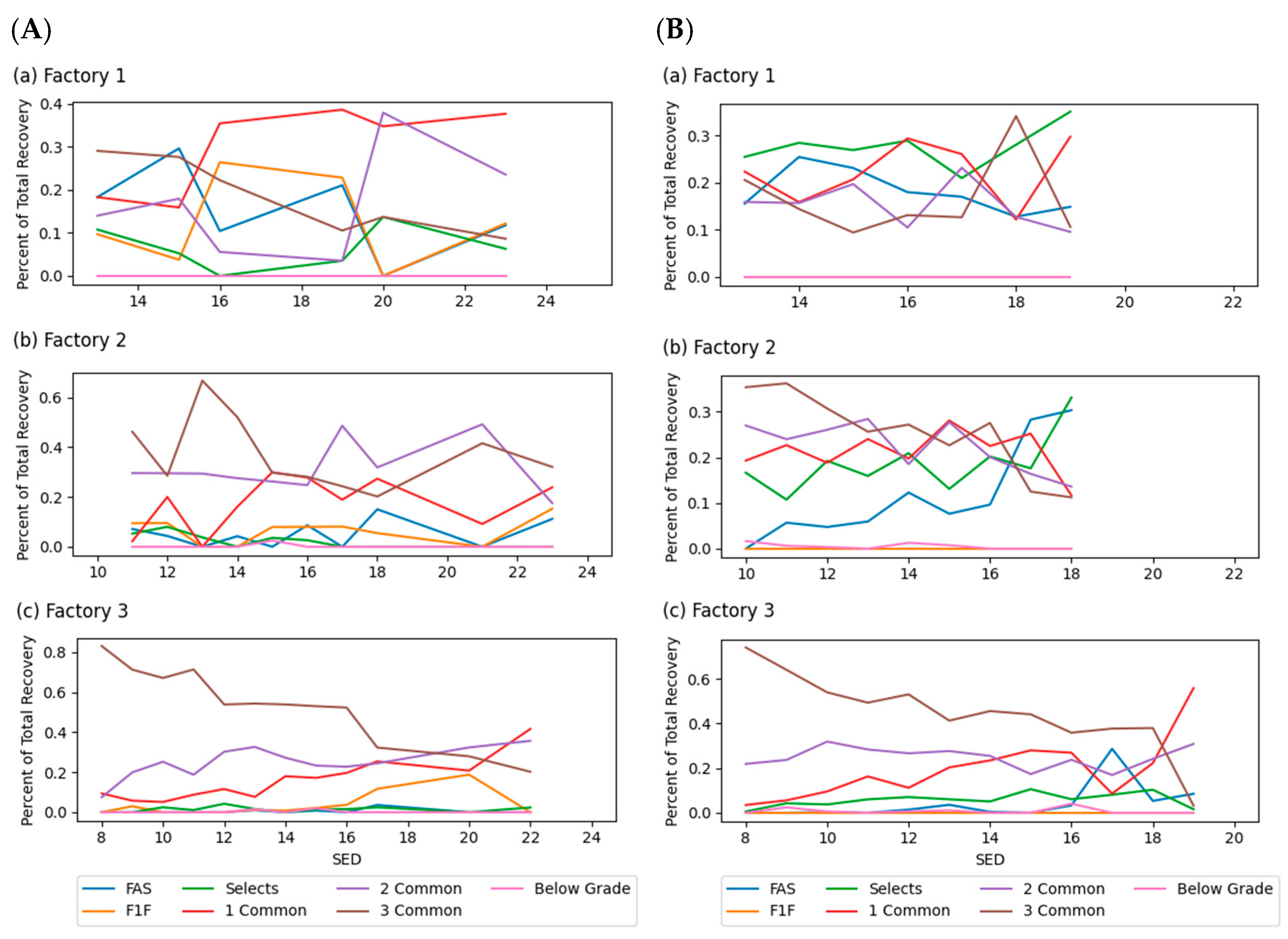
The erratic nature of the recovery data, illustrated in Figure 2 and Figure 3, shows that any model developed to approximate the original data series and smooth the differences between SEDs will necessarily deviate from the original data. Thus, while the goal is to have a model with smooth transitions in NHLA grade recovery between SEDs, due to the erratic nature of the original data, the errors can be high. To minimize this and obtain a model that is as accurate as possible, we used mean absolute error (MAE) as the training evaluation metric.

Table 3. Mean absolute error (MAE) by NHLA lumber grade and USFS log grade for birch and beech validation samples.

NHLA Lumber Grade							USFS
Below	Three	Two	One				Log
Grade	Common			Selects	F1F	FAS	Grade	Species
0.021	0.072	0.126	0.113	0.043	0.086	0.155	1	Beech
0.013	0.155	0.107	0.119	0.034	0.064	0.059	2
0.009	0.152	0.110	0.087	0.018	0.029	0.015	3
0.003	0.073	0.089	0.099	0.095	0.014	0.122	1	Paper Birch
0.010	0.126	0.122	0.104	0.109	0.010	0.082	2
0.020	0.211	0.143	0.117	0.074	0.011	0.033	3

shows the MAE values for the beech and birch samples by USFS log grade and NHLA lumber grade. One should note that the MAE values will be higher for the most frequently sawn NHLA grades, e.g., FAS, 1 Common, 2 Common, and 3 Common, as these will have a greater range of values. This is seen in Table 3, where the minor NHLA grade components of recovery, F1F, Selects, and below grade have a lower MAE than the major NHLA grade recoveries. Overall, the highest MAE observed with birch was 0.211 for Factory grade 3 logs and 3 Common recovery. For beech, the highest MAE, 0.155, was observed with both Factory 1 for FAS recovery, and Factory 2 for 3 Common recovery.

The MAE values shown in Table 3 are reflected in Figure 3, where the average recovery from Hanks et al. [12] is compared to the modeled recovery. The recovery plot comparison for beech and birch Factory 1 logs (Figure 3(Aa) and Figure 3(Ba), respectively) shows an erratic original recovery that is largely due to the small sample size (Table 1). One benefit of using a neural network model is the generalization of trends across the entire data set [21], e.g., all 11,382 logs. For example, the small sample size of beech and birch logs caused the percentage of FAS recovery to decrease as the SED increased (Figure 2(Aa,Ba)), which is counter to the overall recovery trends [12,18]. The generalization capabilities of the neural network corrected the trend and made it compatible with the general trend of hardwood recovery.

The interpretability of a machine learning model is the degree to which a human can understand and predict how the model reaches its decisions. We used the post hoc Shapley Additive exPlanations (SHAP) method for this analysis [22]. SHAP provides a unified measure of feature importance based on cooperative game theory to explain the contribution of each feature to the prediction. As such, the SHAP analysis results are a vector of values associated with each feature that report the average contribution of that particular feature to the overall prediction. The higher the value, the greater the contribution of that feature.

Table 4. The top ten model contributing features and associated mean SHAP values.

Feature	Mean |SHAP| Value
SED	0.0230
Factory 3	0.0131
Factory 1	0.0123
Basswood	0.0097
Red maple	0.0056
Sound log	0.0050
Yellow poplar	0.0048
Factory 2	0.0046
N. red oak	0.0039
Unsound log	0.0032

reports the top ten features and their SHAP values that made the greatest contributions to the model predictions. All the major predictor variables, SED, log grade, and sound or unsound log, made the greatest contributions to the overall prediction, with SED and the log grades Factory 3 and Factory 1 being the most important contributors. However, the species of basswood, red maple, yellow poplar, and northern red oak are also important contributors. Their importance to the prediction indicates that these species would have a greater impact on generalization with respect to species with fewer samples in the model [21]. This observation is key with respect to beech and birch, two species with somewhat fewer observations than others in the database [13]. The generalization capabilities of deep learning neural network models, like TensorFlow, greatly improve the performance of models in areas with a reduced sample size [23] compared to standard neural network methods.

The 3 Common lumber-grade recovery for beech Factory 2 and 3 logs have the highest and next highest MAEs for beech recovery (Table 3), evident in the grade recovery plot comparisons (Figure 3(Ab,Ac)). Beech 2 Common recovery for Factory 2 logs has the third highest MAE (Table 3) and is also illustrated by the erratic averaged recovery plot shown in Figure 3(Ab). Similarly, 3 Common recovery for Factory 3 birch logs has the highest MAE (Table 3), and this is illustrated in Figure 3(Bc).

In the beech and birch samples used, the largest SED logs have the lowest sample counts, regardless of log grade. Thus, the averaged recovery for the larger SEDs plotted in Figure 3 is based on a small sample size, often showing an erratic departure from the normal averaged trend line, either upward or downward, that is attributable to one or more samples that could be regarded as an outlier in traditional statistical methods. However, as in the original study by Hanks et al. [12], these samples were retained in the analysis. Unlike the Hanks et al. study [12], the TensorFlow-based [17] neural network approach automatically de-emphasizes these observations during model creation, allowing a model to be produced that more accurately reflects the overall grade recovery trends of the NHLA grades.

Table 5. Pearson R values by NHLA lumber grade and overall for all species and log grades in the validation dataset.

Pearson		NHLA
Correlation Coefficient		Lumber
p	R	Grade
<0.05	0.68	FAS
<0.05	0.597	F1F
<0.05	0.606	Selects
<0.05	0.498	1 Common
<0.05	0.67	2 Common
<0.05	0.665	3 Common
<0.05	0.366	Below grade
<0.05	0.574	Overall

shows the Pearson correlation coefficients (R) for each NHLA grade from the validation sample of all species (Table 1). The Pearson correlation coefficients were all significant (α = 0.05), with the lowest R value occurring with below-grade recovery (R = 0.366) and the highest with FAS recovery (R = 0.680, Table 5).

Using the LORCAT sawing simulator [2], a sample consisting of 25 Factory 1 and 40 Factory 2 grade beech logs was created. These log grades are somewhat like the logs graded using EN 1316-1 [24] and other regional grades used in Europe. However, the transferability of LORCAT’s results is indicative rather than direct due to LORCAT’s use of North American species, grading systems, and economic assumptions, including species properties and distributions, log and lumber grading systems, measurement systems, cost structures, and the economic framework.

The sample was designed to replicate a potential harvest with lower-grade logs culled. As the Factory 1 grade logs are more often butt logs, they exhibit more taper and have a larger SED than upper logs. We replicated this by creating a sample where the Factory 1 logs had a 50 mm larger average SED than the Factory 2 logs (550 mm versus 500 mm), and with the Factory 1 logs having an average mean taper that was 25 mm greater than the Factory 2 logs (100 mm versus 75 mm). Lastly, all logs were 4 m long. Overall, the sample contained 29.9 m³ and 36.3 m³ of logs for the Factory 1 and Factory 2 grades, respectively.

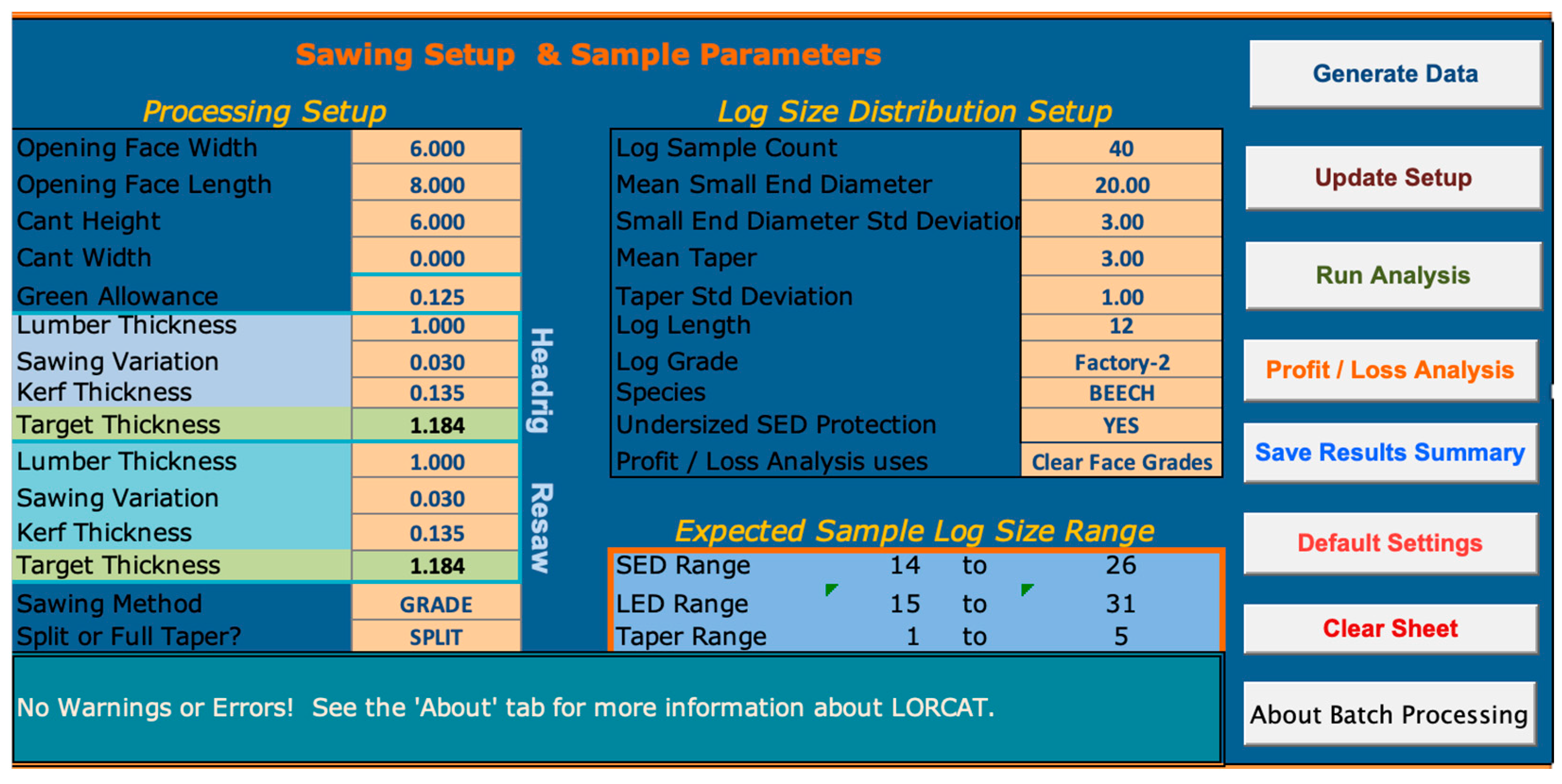
The sawing simulation was designed to replicate the North American process of grade sawing to a cant 150 mm thick, where the cant was subsequently gang sawn into lumber. For sawing, we specified a board thickness of 25 mm and a kerf of 3.44 mm, with a total sawing variation of 0.76 mm. The same kerf and total sawing variation parameters were used on the headrig and resaw. A minimal opening face width of 150 mm and length of 2.4 m were used for sawing, corresponding to the minimum board size required for FAS lumber (NHLA). Figure 4 shows the details of the settings for this simulation run.

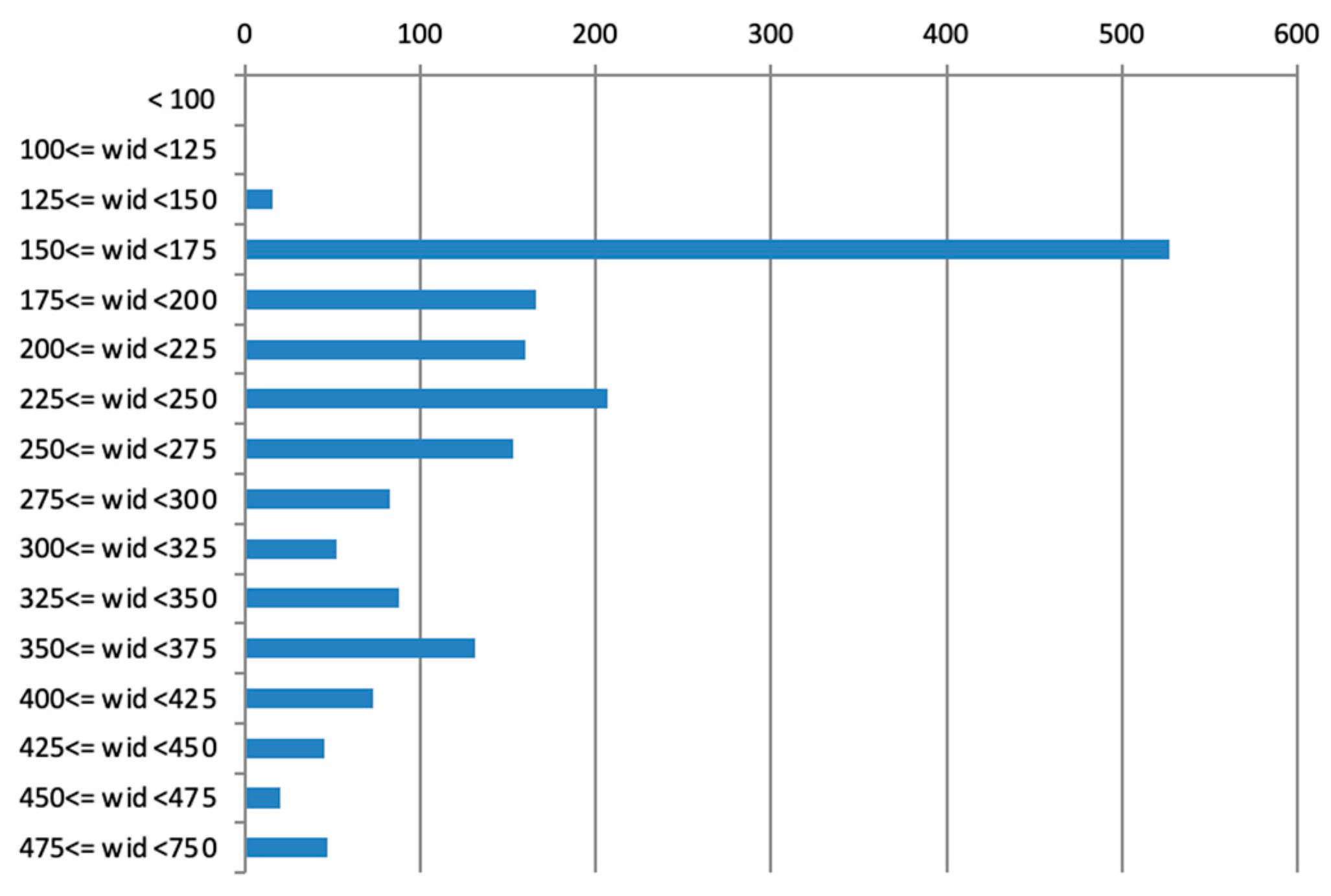
Overall, a total of 39.81 m³ of lumber (60.1% yield), 18.09 m³ and 21.72 m³ from Factories 1 and 2, respectively, was sawn from 66.25 m³ of logs. Figure 5 shows the board width distribution summary for all the boards generated in this sample simulation. As the cant was set to 150 mm, more than 500 boards produced were of this size. However, as seen in Figure 5, boards of up to 475 mm to 750 mm were also produced, albeit in small numbers.

A current limitation of LORCAT is the sole use of the National Hardwood Lumber Association (NHLA [9]) grading rules used to classify the resulting lumber. NHLA standards can roughly be translated into the official European Standard, EN 975-1 [25], where FAS and F1F are A1, Selects and 1 Common are A2, borderline 1 Common and 2 Common are A3, and A4 is 3 Common or below grade [26]. A greater volume of the higher grades, FAS, F1F, and Selects, was sawn using the Factory 1 logs despite it being the smaller log sample (

Table 6. Lumber produced by NHLA grade for each log grade and total.

Total (m3)	Factory 2 (m3)	Factory 1 (m3)	Lumber Grade
4.42	0.94	3.48	FAS
2.89	0.91	1.98	F1F
1.72	0.59	1.12	Selects
9.81	5.37	4.44	1 Common
9.47	6.25	3.22	2 Common
10.99	7.41	3.58	3 Common
0.52	0.26	0.27	Below grade

). This is a good illustration of the difference in quality between the two log grades, Factory 1 vs. Factory 2. In addition, greater volumes of lower-grade lumber, 1 Common, 2 Common, and 3 Common, were sawn using the Factory 2 logs versus the Factory 1 logs. The volume differences between log grades for the lowest lumber grades, 2 and 3 Common, are especially pronounced, with the Factory 2 volumes reaching approximately twice that of the Factory 1 logs. The volume of below-grade lumber was approximately the same between the Factory 1 and Factory 2 log samples.

A total of 80.3 m³ of residues (chips, sawdust, bark), weighing approximately 27.9 tons, were produced.

Table 7. Residues (chips, sawdust, and bark) in tons and volume produced in simulation.

		Weight	Volume
Total	Factory 2	Factory 1	Total	Factory 2	Factory 1
(kg)	(kg)	(kg)	(m3)	(m3)	(m3)	Residue
19,013.1	10,569.1	8444	53.5	29.7	23.7	Chips
7872.6	4294.6	3578	19.3	10.6	8.8	Sawdust
1021.8	596.3	425.5	7.5	4.4	3.1	Bark
27,907.6	15,460	12,447.6	80.3	44.6	35.7	Total

shows the residues in m³ and tons for the different log grades (Factory 1 and Factory 2) and the total for chips, sawdust, and chips. LORCAT first calculates the volumes of residuals as solid volumes that are subtracted from the total log volume, less the volume of lumber sawn. Expanded volumes are then calculated from the solid volumes based on known expansion factors for chips, sawdust, and bark [27]. Weights for residues are calculated at the moisture fiber saturation points of beech and birch using published weights for the species [27]. LORCAT allows users to modify both the expansion factors and residue weights if they do not feel that they are reflective of their operation. In addition, users can specify an average measurement for debarker overgrind to adjust the settings to their situation or if they want to demonstrate the recovery impact on lumber and residues.

The Log Recovery Analysis Tool (LORCAT) software [2] allows users to simulate their own operation and obtain estimates of the lumber and residues they can expect. Thanks to the new model, estimating the expected lumber-grade distribution (NHLA grades [9]) from the logs sawn provides users with the opportunity to estimate the profitability of the sawing they are about to undertake.

LORCAT [2] can now saw beech (Fagus grandifolia) and paper birch (Betula papyrifa) based on the work by Rast et al. [11] and Hanks et al. [12]. Currently, LORCAT (Version 4.2) saws red oaks (Quercus rubra, velutina, and coccinea, falcata), white oaks (Quercus alba, macrocarpa, lyrata, and montana), soft maple (Acer rubrum and saccharinum), hard maple (Acer saccharum), yellow poplar (Liriodendron tulipifera), beech (Fagus grandifolia), and paper birch (Betula papyrifa) based on Hanks et al.’s [12] study. However, the model presented in this manuscript has not been validated with actual sawing studies; it relies entirely on the work by Rast et al. [11], Hanks et al. [12], and Wood et al. [13]. Future work will have to demonstrate the accuracy and reliability of the model’s predictions. Also, additional work could add more data to the recovery model of NHLA grade lumber [9] based on the log grade and small-end diameter to increase the statistical validity of the results.

4. Conclusions

Using the Log Recovery Analysis Tool (LORCAT) software, industry participants and researchers can simulate the sawing of 13 common North American hardwood species (red oak, white oak, scarlet oak, chestnut oak, red maple, sugar maple, yellow poplar, paper birch, yellow birch, black cherry, basswood, and American beech), with beech (Fagus grandifolia) and paper birch (Betula papyrifa) having been added to the mix, as described in this manuscript. A neural network was used to model these species based on work conducted by Rast et al. [11], Hanks et al. [12], and Wood et al. [13], using their recordings of grade recovery by NHLA grades [9] for Factories 1, 2, and 3 logs, graded according to Rast et al. [11].

Using species, log grade [11], scaling diameter, and a scaling deduction indicator (for deficiencies of a log) [12], the neural network used data for 25 hardwood species and three log grades, with a total of 11,382 logs, to model the yields of FAS, F1F, Selects, 1 Common, 2 Common, 3 Common, and below NHLA specifications [9] lumber from sawing the logs. Eighty percent of the data were used for training and 20 percent for validation. The model achieved an overall Pearson correlation coefficient of 0.57, with the lumber that was graded below grade having the lowest coefficient at 0.37. First and Second (FAS) grade had a Pearson correlation coefficient of 0.68, followed by 2 Common, 3 Common (both 0.67), and Selects (0.61), followed by FAS-1-Face (F1F) with 0.60, and 1 Common with 0.50. All correlation coefficients were statistically significant (p < 0.05).

Using this model, we sawed 25 Factory 1 and 40 Factory 2 logs, with the Factory 1 logs having a larger small-end diameter (SED) than the Factory 2 logs (average 50 mm larger) and Factory 1 having more taper (average 25 mm). All logs sawn were 4 m long, for a total log volume of 29.9 m³ and 36.3 m³ for Factory 1 and Factory 2, respectively. The logs were sawn to 25 mm dried thickness (30 mm sawn), with a 150 mm cant subsequently sawn into lumber and a kerf of 3.4 mm and a total sawing variation of 0.8 mm.

A total of 39.8 m³ of lumber was sawn for a total of 1768 boards, with 527 between 150 mm and 175 mm wide (due to the cant size). Factory 1 logs created 3.5 m³ of FAS lumber (NHLA-graded), while Factory 2 contributed only 0.9 m³ for a total of 4.4 m³. Despite sawing fewer Factory 1 logs than Factory 2 logs (29.9 m³ vs. 36.3 m³), Factory 1 logs produced more higher graded lumber (FAS, F1F, Selects) than Factory 2. A total of 80.3 m³ (27,908 kg) of residues were produced, with 53.5 m³ (19,013 kg) of chips, 19.3 m³ (7873 kg) of sawdust, and 7.5 m³ (1022 kg) of bark produced, respectively.

Unfortunately, due to money constraints, the model has not yet been validated. Future research should focus on validating the model created for beech and birch sawing. Furthermore, all these species’ yields are based on a dry lumber model (neural network); data exist for a lumber yield model for green lumber. LORCAT [2] is a free tool that helps industry practitioners and researchers investigate scenarios for sawing hardwood lumber for increased profitability. LORCAT can be used to investigate the resulting products from a given input of logs to assess the pricing of these products and the profitability of users’ operations.