


Abstract
Karst Mountain Areas (KMAs) are characterized by fragile geology, shallow soils, and high ecological sensitivity, rendering their Ecosystem Services (ESs) highly vulnerable to Land Use and Land Cover (LULC) change. However, the spatiotemporal evolution of ESs and the trade-offs and synergies among them remain poorly understood, particularly concerning the interplay between human activities and natural constraints in these complex landscapes. Taking the Wumeng Mountain Area (WMA) in southwestern China as a representative case, this study integrates multi-temporal LULC data (2000, 2010, and 2020) with the InVEST model to quantify the dynamics of four key ESs: Carbon Storage (CS), Habitat Quality (HQ), Soil Conservation (SC), and Water Yield (WY). An integrated analytical framework combining land use dynamic degree, intensity analysis, transition matrices, and grid-scale Spearman correlation analysis was developed to reveal ESs interactions. Results indicate that, despite substantial land use changes, most ES pairs exhibited synergistic relationships, and these synergies intensified from 2000 to 2020. The strengthened synergies, particularly among CS, SC, and HQ, are conducive to simultaneously achieving multiple ecological security goals, such as regional carbon sequestration, biodiversity conservation, and soil stability. However, the trade-offs observed between water yield and regulating services (CS, HQ) in 2000 highlight potential conflicts between ensuring water supply and enhancing other ecological benefits in fragile karst landscapes, offering a scientific caution for balancing water resource development with ecological protection. This study demonstrates that understanding ES interactions is not merely an ecological description but constitutes a critical scientific basis for optimizing land use and improving regional human well-being and sustainability.
1. Introduction
Ecosystem Services (ESs) refer to the benefits that humans derive directly or indirectly from ecosystem structures, processes, and functions, and they constitute a fundamental basis for human well-being and sustainable development [1,2]. Harrington et al. [3] working within the RUBICODE project, further developed this conceptual framework by unifying the concepts of the Service-Providing Unit (SPU) and Ecosystem Service Provider (ESP) into an SPU-ESP continuum, thereby providing operational definitions for quantifying how the characteristics of organism and habitats contribute to service delivery. In recent decades, accelerating Land Use and Land Cover (LULC) change, driven by urbanization, agricultural intensification, and infrastructure expansion, has profoundly altered ecosystem processes and the provision of ESs worldwide [4,5]. Understanding how ESs respond to LULC change and how different services interact with one another has therefore become a central issue in ecological and geographical research.
Karst Mountain Areas (KMAs) represent some of the most ecologically fragile landscapes on Earth. Owing to their distinctive geological and geomorphological features—including soluble carbonate bedrock, shallow and discontinuous soils, strong surface-subsurface hydrological connectivity, and high spatial heterogeneity-karst ecosystems exhibit limited ecological resilience and heightened sensitivity to external disturbances [6,7]. Once degraded, ecosystem recovery in KMAs is often difficult to reverse, posing serious challenges to ecological security and sustainable regional development [8,9]. However, following the launch of China’s reform and opening-up policy, and concomitant with the rapid pace of urbanization and industrial growth, urban construction land has undergone continuous expansion. Furthermore, unsustainable land use practices have further damaged the natural ecological environment in KMAs, intensifying the conflict between human activities and environmental capacity. Specifically, the decline in soil and water conservation services may lead to the loss of fertile topsoil, accelerate the desertification of farmland, impair agricultural productivity, and threaten regional food security and farmers’ livelihoods. The degradation of habitat quality can also deplete biological resources that depend on specific ecosystems, compromising the sustainable supply of valuable medicinal plants and local specialty products, thereby undermining the livelihood sources of certain communities. In addition, the high spatiotemporal variability of water yield increases the risk of both droughts and floods, which can pose a serious threat to agricultural irrigation in mountainous areas and to the drinking water security of rural populations and livestock that rely on stable water supplies. These pressures have resulted in varying degrees of degradation in both the quantity and quality of ESs in KMAs, causing ecosystem management and restoration in these regions to face substantial challenges [10]. According to the Millennium Ecosystem Assessment (MEA) conducted by the United Nations in 2005, approximately 60% of global ESs were facing degradation, posing a significant threat to regional and global ecological security [11]. This finding was further substantiated and updated by the Intergovernmental Science-Policy Platform on Biodiversity and Ecosystem Services (IPBES), whose 2019 Global Assessment Report concluded that the majority of ESs worldwide have continued to decline [12]. Therefore, analyzing the long-term changes in ESs within KMAs has become a key focus and a prominent research frontier in contemporary science.
Previous studies have developed a wide array of approaches to quantify ESs, which can be broadly categorized into value-based assessments and process-based or biophysical assessments [13]. Compared with equivalent factor methods, process-based models offer greater explanatory power by explicitly representing ecological mechanisms [14,15]. Among the available modeling tools, the InVEST (Integrated Valuation of Ecosystem Services and Trade-offs) framework has been extensively applied to assess regulating and supporting services such as Carbon Storage (CS), Habitat Quality (HQ), Soil Conservation (SC), and Water Yield (WY) across diverse spatial scales [16,17]. Nevertheless, most existing studies have focused on plains, river basins, or urban agglomerations, whereas comprehensive assessments in KMAs remain relatively scarce.
Beyond quantifying individual ESs, increasing attention has been directed toward the interactions among different ESs [18,19]. Owing to the spatial heterogeneity of natural conditions and the differentiated impacts of human activities, ESs often exhibit complex relationships characterized either by synergies—where multiple services increase or decrease simultaneously—or by trade-offs—where the enhancement of one service leads to the degradation of another [20,21]. Exploring these trade-off and synergy relationships is essential for identifying ecological management priorities and mitigating conflicts between socioeconomic development and environmental protection. Previous research has employed methods such as spatial overlay analysis [22], correlation analysis [23], scenario simulation [24,25], and other methods to investigate ESs interactions [26]. However, in KMAs, where ecological processes are strongly constrained by natural conditions, the spatial and temporal patterns of synergies and trade-offs among ESs, as well as their driving mechanisms, remain insufficiently understood.
Land use change constitutes a key pathway through which human activities influence ESs. Urban expansion, ecological restoration projects (e.g., returning farmland to forest or grassland), and water conservancy infrastructure development can directly reshape land use patterns and indirectly alter ecosystem functions. In KMAs, these impacts may be further amplified by hydro-climatic variability and fragile soil-vegetation systems. Existing studies often emphasize either human-driven LULC change or natural environmental factors in isolation [27], whereas relatively few have examined their combined effects on ESs and ES interactions within a unified analytical framework.
The Wumeng Mountain Area (WMA), located within this climatic context, represents a typical KMA characterized by complex terrain, high ecological sensitivity, and pronounced human-land conflicts [28]. In recent decades, the WMA has undergone rapid urbanization and large-scale ecological restoration, accompanied by substantial land use transitions. These characteristics render the WMA an ideal case for investigating the spatiotemporal dynamics of ESs and their associated trade-off and synergy relationships.
Nevertheless, the spatiotemporal patterns of synergies and trade-offs among ESs and their driving mechanisms remain poorly understood in typical KMAs such as the WMA, particularly with respect to the inherent stability of ES interactions under the superimposed influences of natural conditions and human activities. This constitutes a critical research gap. To address this gap, this study focuses on four ESs that are pivotal to karst ecological security and human well-being: CS, HQ, SC, and WY. These services correspond to the core dimensions of socio-ecological resilience, including regional climate mitigation, biodiversity maintenance, soil retention and agricultural productivity, and water resource supply. Accordingly, this study integrates multi-temporal LULC data from 2000, 2010, and 2020 with the InVEST model to systematically analyze ESs dynamics in the WMA. Specifically, this study addresses the following key questions: (1) How have LULC patterns in the WMA changed over the past two decades? (2) How have key ESs—CS, HQ, SC, and WY—responded to these land use changes? (3) What are the spatiotemporal characteristics of trade-offs and synergies among these ESs? By answering these questions, this study seeks not only to achieve an ecological understanding of ES interactions but also to elucidate the specific decision-making support that such interactions can provide for optimizing territorial spatial planning, deploying ecological restoration projects, and managing water resources in KMAs.
2. Materials and Methods
2.1. Study Area
The WMA lies in the transitional belt between the Yunnan-Guizhou Plateau and the Sichuan Basin in southwestern China, serving as a vital ecological security barrier for the upper reaches of the Yangtze and Pearl Rivers [29]. Encompassing 38 county-level administrative units across the junction of Yunnan, Sichuan, and Guizhou provinces, the region extends from 25.3° N to 29.3° N latitude and from 101.9° E to 107.3° E longitude, covering a total area of approximately 106,300 km2 (Figure 1). Tectonically, the WMA is situated at the boundary between the Tethys-Himalayan and Pacific coastal systems, stretching over 600 km in a northeast-southwest orientation. It represents a typical plateau-mountain karst landscape. Karst features underlie approximately 52.75% of the total area. The landscape exhibits a complex and varied assemblage of karst formations with significant bedrock exposure. Dominant soil types include red soils and limestone soils, which are typically characterized by low fertility.
Figure 1.
Study area map. (a) Provincial boundaries and location of the study area; (b) DEM distribution of the WMA in 2020; (c) Land use distribution of the WMA in 2020.
Climatically, the WMA experiences a mid-subtropical plateau monsoon climate combined with warm-temperate humid monsoon influences. The mean annual temperature ranges from 11 °C to 18 °C, and total annual precipitation generally exceeding 900 mm. However, pronounced spatial heterogeneity exists in both precipitation and evapotranspiration. Mean annual precipitation decreases from southeast to northwest, whereas potential evapotranspiration is higher in the northwestern sectors than in the southeast. This spatial variability in hydrothermal conditions strongly governs vegetation distribution and ESs patterns across the region. Correspondingly, the vegetation exhibits notable diversity with clear vertical zonation. The forest cover rate is approximately 40%; however, the area is severely affected by rocky desertification, rendering its ecological environment highly sensitive. According to the Seventh National Population Census, the region supports a population of 19.38 million. Key challenges include limited per capita arable land, low-quality farmland, and acute land use conflicts.
2.2. Data Sources
All datasets employed in this study encompass six categories, with detailed information provided in Table 1.
Table 1.
Datasets used, their sources, and brief descriptions.
Table 1 summarizes the six categories of data used in this study. Detailed descriptions are provided as follows. LULC data for 2000, 2010, and 2020 were obtained from the GlobeLand30 repository (https://www.un-spider.org/links-and-resources/data-sources/land-cover-map-globeland-30-ngcc, last accessed on 1 May 2025). This dataset provides ten land cover classes—cultivated land, forest, grassland, shrubland, wetland, water bodies, tundra, artificial surfaces, bare land, and glaciers/permanent snow—at a 30 m spatial resolution, with an overall reported accuracy exceeding 85%. Annual precipitation data for the same three years were acquired from the national annual average precipitation dataset hosted by the Earth Resources Data Cloud Platform (www.gis5g.com, accessed on 16 May 2025), at a resolution of 1 km. Monthly potential evapotranspiration (PET) data were retrieved from the China monthly PET dataset distributed by the National Tibetan Plateau Scientific Data Center (https://data.tpdc.ac.cn, accessed on 24 May 2025), which was derived using the Hargreaves method and is provided at a 1 km resolution. Soil property information was extracted from the Harmonized World Soil Database (HWSD) via the Resource and Environmental Science Data Platform of the Chinese Academy of Sciences (https://www.resdc.cn, accessed on 25 May 2025), also at 1 km resolution. A Digital Elevation Model (DEM) was sourced from the ASTER Global Digital Elevation Model dataset available on the Geographic Spatial Data Cloud platform (https://www.gscloud.cn, accessed on 25 May 2025), with an original resolution of 30 m. Administrative vector boundaries of the study area were downloaded from the TianDiTu service (https://sso.tianditu.gov.cn, accessed on 25 May 2025). To establish a consistent analytical foundation, all raster datasets were resampled to a uniform 30 m spatial resolution using ArcGIS Pro 3.1 software (Esri, Redlands, CA, USA). Monthly PET values were aggregated to generate annual totals for each corresponding year. Based on these preprocessed datasets, this study analyzed the spatiotemporal evolution of LULC and ESs in the WMA—a typical KMA—from 2000 to 2020, as well as the complex synergy and trade-offs relationships among ESs.
2.3. Methods
The overall analytical framework of this study is schematically illustrated in Figure 2, which outlines four key components: (a) methods for analyzing the spatiotemporal evolution of LULC; (b) quantification approaches for assessing the spatiotemporal dynamics of four ESs; (c) methods for analyzing synergy–trade-off relationships among ESs; and (d) the analysis of driving factors, encompassing both natural and anthropogenic dimensions. Detailed formulations for the corresponding models and indices are presented in the following sections.
Figure 2.
Technique roadmap.
2.3.1. Land Use Dynamics
Land use dynamics refers to the magnitude and direction of change in LULC types over a defined period. Change rates vary across different LULC types owing to the combined influence of natural processes and anthropogenic activities. To quantify these changes, this study employs two complementary metrics: the single land use dynamic degree (for individual LULC types) and the comprehensive land use dynamic degree (for an integrated assessment at the regional level). The calculation formulas are presented below [30]:
where D denotes the dynamic degree of single type of land use; Ua and Ub represent the area of the land use type at the initial and final time points, respectively; T is the time interval corresponding to the observed change; LCd is the comprehensive land use dynamic degree for the entire region; and refers to the absolute value of the area of land use type i that was converted to other, non-i land use types during the period T.
The underlying assumption of these indicators is that land use changes are predominantly driven by human activities (e.g., urbanization, agricultural expansion, ecological restoration) rather than by natural successional processes, given the relatively short study period (20 years) and the high intensity of anthropogenic modification within the WMA. The single dynamic degree (D) assumes that the net change of a given land use type reflects the balance between gains (i.e., conversions into that type) and losses (i.e., conversions out of that type). A positive value of D indicates net expansion, whereas a negative value signals net contraction. The comprehensive dynamic degree (LCd) captures the overall turnover intensity of the entire land use system, irrespective of whether individual types are expanding or shrinking. Together, these indicators provide a quantitative basis for assessing the pace, direction, and magnitude of land use change. In terms of land use practices, a persistently high LCd (e.g., 7.11% over the period 2000–2020 in the WMA) suggests a landscape undergoing rapid and widespread reorganization, implying that human interventions—such as urban sprawl, reservoir construction, and the Grain-for-Green program—are actively reshaping the spatial configuration of land use. Conversely, a low LCd would indicate relative stability or path dependency. By linking these dynamics to the subsequent ESs analysis, it is possible to evaluate whether observed land use transitions have led to improved ecosystem service provision (i.e., synergies) or unintended trade-offs.
2.3.2. Land Use Intensity
Different land use types correspond to varying degrees of anthropogenic modification of the natural environment and thus serve as indicators of land development and utilization intensity. Land use intensity quantifies this degree of anthropogenic transformation [31]. A higher land use intensity value signifies a greater overall intensity of land use within a region, which concurrently reflects a higher level of human activity and a more pronounced anthropogenic impact on the natural environment. The different land use types are assigned the following intensity indices: construction land is assigned an index of 4, agricultural land (cultivated land) has an index of 3, ecological land (forest, grassland, shrubland, wetland, water bodies) has an index of 2, and unused land (bareland, permanent snow and ice) has an index of 1. The overall land use intensity index is calculated as follows:
where S denotes the land use intensity of a given region-the higher the value of S, the greater the overall land use intensity in the region, indicating a higher level of human activity and alteration of the natural environment. Ti is the land use intensity index corresponding to the i-th land use patch; Ai refers to the area of the i-th land use patch; A is the total area of all land use patches in the region; n is the total number of land use patches in the region.
2.3.3. Land Use Transition Matrix
The land use transition matrix is a quantitative tool for analyzing the direction and magnitude of conversions among different LULC types. It delineates the specific pathways of change between LULC categories and facilitates the analysis of structural characteristics underlying land use change [32]. The matrix is represented in the following mathematical form:
where M denotes the land use transition matrix; n is the total number of land use types considered in the analysis; i and j represent the land use types before and after the study period, respectively; Mij represents the area of land that transitions from land use type i to land use type j.
2.3.4. Spatiotemporal Evolution Characteristics Analysis Methods of ESs
Linking ES indicators to karst-specific challenges. To clarify the role of KMAs in this analysis, each selected ES indicator is explicitly linked to the distinctive environmental problems of KMAs identified in the Introduction. (1) Carbon Storage (CS) is particularly critical in KMAs because shallow, discontinuous soils and rocky desertification limit organic matter accumulation; thus, CS reflects the capacity of vegetation and soil to sequester carbon under karst constraints. (2) Habitat Quality (HQ) addresses the high ecological sensitivity of karst landscapes, where habitat fragmentation and biodiversity loss are exacerbated by thin soils and hydrological isolation. (3) Soil Conservation (SC) directly responds to the severe soil erosion and rocky desertification typical of KMAs; the thin soil layer renders soil retention a priority for preventing irreversible degradation. (4) Water Yield (WY) captures the unique surface-subsurface hydrological connectivity of karst systems, where rapid infiltration and underground drainage lead to complex water availability patterns. By assessing these four services, this study aims to capture the most vulnerable aspects of karst ecosystems. Moreover, the analysis of trade-offs and synergies among these services helps reveal whether land use changes and restoration efforts in KMAs lead to mutually beneficial outcomes (e.g., simultaneous increases in CS and SC) or unintended conflicts (e.g., WY increases at the expense of HQ). Thus, the karst context is not merely a geographic label but is embedded in both the selection of indicators and the interpretation of results.
The Integrated Valuation of Ecosystem Services and Tradeoffs (InVEST) model is a spatially explicit tool designed for mapping, modeling, and valuing ESs. Developed through a collaboration between Stanford University, The Nature Conservancy, and the World Wildlife Fund, the model enables the assessment of both the biophysical supply and the economic value of ESs. It has been extensively applied in diverse ecosystems worldwide. It is important to note, however, that the accuracy of InVEST outputs is contingent upon the quality of input data and the local calibration of model parameters. Given the ecological sensitivity and severe rocky desertification prevalent in the study area, and in alignment with methodologies established in prior research [33], this study employs the InVEST model to quantitatively assess four key ESs: CS, HQ, SC, and WY.
- (1)
- CS
Ecosystem CS comprises four primary carbon pools: aboveground biomass, belowground biomass, soil organic matter, and dead organic matter [34]. For this study, carbon density parameters corresponding to different LULC types were compiled from published literature focusing on the WMA and analogous regions. This compilation enabled the construction of a localized carbon density parameter set tailored to the study area. The InVEST model’s Carbon Storage and Sequestration module was subsequently applied to estimate total ecosystem CS across the WMA. The underlying calculation is based on the following formula:
where C denotes the total carbon storage of the ecosystem; CAbove is the aboveground biomass carbon pool; CBelow is the underground biomass carbon pool; CSoil is the soil organic carbon pool; CDead is the dead organic matter carbon pool.
Based on the land use type data and the carbon density data for different land use types, the CS in each carbon pool type within the study area can be calculated as follows:
where Ci is the total carbon storage of the i-th carbon pool in the ecosystem (e.g., aboveground biomass carbon, belowground biomass carbon, soil organic carbon, or dead organic matter carbon); Cij is the carbon density parameter for the i-th carbon pool in the j-th land use type (expressed in tons of carbon per hectare or per square kilometer); Aj is the total area of the j-th land use type (in hectares or square kilometers); n is the total number of land use types considered in the study.
This study constructed a localized carbon density parameter set (Table 2) by extensively reviewing published literature [35,36] and integrating field survey data collected by our project team within the WMA.
Table 2.
Assigned carbon density values by LULC type (t/hm2), where hm2 denotes hectare (1 hm2 = 10,000 m2).
- (2)
- HQ
The HQ module within the InVEST model estimates habitat quality by integrating two key components: the intensity of external threats and the inherent sensitivity of the landscape to those threats. Drawing on related studies [37,38], the study considers cropland, construction land, and unused land as threat factors for the HQ assessment. The sensitivity of each habitat type to these threat factors and the corresponding habitat suitability scores are detailed in Table 3. The maximum influence distance and assigned weight for each threat source are set as follows: for cultivated land, construction land and unused land, the maximum influence distances are 4 km, 10 km and 2 km, respectively; the weight values are 0.6, 1.0, and 0.5; and the decay types are all exponential. The core calculation is governed by the following equation:
where Dxj is the habitat degradation degree for the x-th grid cell and j-th habitat type; r indexes the threat source, and R is the total number of external threat sources; denotes the weight of the r-th threat source; Yr is the number of grid cells affected by the r-th threat source; is the intensity or threat level of the r-th threat source at a given grid cell; is the accessibility factor of the x-th grid cell to the threat source (reflecting the ease with which the threat source can impact the grid cell); is sensitivity of habitat j to the r-th threat source; is the impact of the r-th threat on the x-th grid cell, which may follow either a linear or an exponential decay model.
Table 3.
Sensitivity of habitat types to threat sources and corresponding habitat suitability scores.
- (3)
- SC
The Sediment Delivery Ratio module in the InVEST model, which is grounded in the Revised Universal Soil Loss Equation (RUSLE), quantifies potential and actual soil erosion to assess SC [39]. The core relationship is expressed by the following equation:
where RKLS denotes potential soil erosion, USLE represents actual soil erosion, and SEDR indicates the amount of intercepted sediment, with the calculation formula as follows:
where R represents the rainfall erosivity factor; K is the soil erodibility factor; LS is the slope length and steepness factor; C is the cover and management factor; P is the support practice factor; and SE is the sediment retention efficiency.
- (4)
- WY
The WY module in the InVEST model employs the Budyko hydrothermal coupling framework together with long-term average annual precipitation data within a water balance approach to quantify water yield. The fundamental principle involves solving the water balance for a given area, where water yield is determined as the residual of precipitation minus actual evapotranspiration [40]. The governing equation for the module is as follows:
where is the water yield (in mm/year); is the actual evapotranspiration (in mm/year); and is the annual average precipitation (in mm/year). The detailed calculation formulas are as follows:
where is the dimensionless aridity (dryness) index that characterizes the dry/wet balance of the climate; is a non-physical empirical parameter that accounts for soil and climate conditions, typically derived from field studies; is the rainfall characteristic coefficient, which adjusts for the effectiveness of rainfall in replenishing soil moisture; is the evapotranspiration coefficient that scales potential evapotranspiration according to local vegetation and climate conditions; is the potential evapotranspiration, typically calculated based on temperature, radiation, or other climate variables; and is the plant available water capacity, i.e., the amount of water in the soil that is available to plants, derived from soil texture and structure. , , and denote the soil composition, representing the contents of sand, silt, clay and organic matter in the soil, respectively.
2.3.5. ESs Synergy–Tradeoff Characteristics Analysis Method
Existing studies have demonstrated that correlation analysis is a widely used method for examining synergies and trade-offs among ESs [41]; however, its application presupposes that the data are normally distributed. In this study, all four ESs (CS, HQ, SC, and WY) exhibited significant deviations from normality across the three study years. Specifically, CS and HQ values displayed right-skewed distributions (positive skewness), with a large number of low-value grid cells and a long tail of high-value cells concentrated in forested areas. SC and WY exhibited multimodal and spatially clustered distributions owing to the strong influences of precipitation, topography, and land use patterns. Such non-normal distributions are common in ecosystem service assessments because of spatial autocorrelation, zero-inflated values (e.g., water yield in non-vegetated areas), and bounded ranges (e.g., habitat quality constrained between 0 and 1). Accordingly, this study employs Spearman’s rank correlation coefficient, using R 4.3.0 software (R Core Team, Vienna, Austria) to calculate the rank correlation coefficients and produce spatial maps at a 1 km grid resolution. Spearman’s rank correlation analysis is a commonly employed and effective method in this research field, as it is capable of identifying linear or monotonic synergistic/trade-off relationships among ESs. It should be noted, however, that this method primarily captures pairwise statistical associations and has limited capacity to reveal nonlinear interactions or causal relationships among multiple services. Nevertheless, given that this study aims to preliminarily elucidate the fundamental patterns of ESs relationships in the WMA, this method remains adequate to address the stated research objectives. The calculation formulas are as follows:
where denotes the Spearman rank correlation coefficient between two ESs; xi and yi are the rank values of each pair of samples for the two ESs, with a total of n sample pairs; and di is the rank difference for the corresponding sample pair.
2.3.6. Hot Spot Analysis (Getis-Ord Gi*)
To identify the spatial clustering patterns of ESs (i.e., cold spots and hot spots), this study employed the Getis-Ord Gi* statistic, a widely used measure of local spatial autocorrelation. Unlike the global Moran’s I, which assesses overall spatial clustering, the Gi* index detects localized clusters of high or low values and evaluates their statistical significance. This method is particularly suitable for revealing the spatial heterogeneity of ESs and for linking the spatial distribution of ESs to underlying drivers such as land use change and hydroclimatic variability [42,43].
The Getis-Ord Gi* statistic is calculated for each grid cell i as follows:
where xj is the attribute value (e.g., CS, HQ, SC, or WY) of grid cell j; wi,j is the spatial weight between cell i and cell j, defined using a fixed distance band (here set to 1 km, consistent with the grid resolution and preceding correlation analysis); n is the total number of grid cells; is the mean of all xj values across the study area; and S is the standard deviation of all xj values. The resulting statistic is a Z-score. Positive and statistically significant Z-scores indicate hot spots (i.e., spatial clusters of high ES values), whereas negative and statistically significant Z-scores indicate cold spots (i.e., spatial clusters of low ES values). A significance level of p < 0.05 was adopted to identify statistically robust cold and hot spots. In this study, the classification of cold spots and hot spots is grounded in rigorous statistical criteria. A grid cell exhibiting a significantly positive Z-score (Z > 1.96, p < 0.05) is designated as a hot spot, signifying a spatial cluster of high ES values. Conversely, a significantly negative Z-score (Z < −1.96, p < 0.05) is classified as a cold spot, representing a spatial cluster of low ES values. This method detects local spatial autocorrelation based on distance weights, rather than relying on simple percentile thresholds or standard deviation classifications, thereby ensuring the statistical rigor and reproducibility of the hot spot analysis.
In this study, the Getis-Ord Gi* index was calculated for each of the four ESs (CS, HQ, SC, WY) in the WMA for the years 2000, 2010, and 2020 using ArcGIS Pro 3.1 software (Esri, Redlands, CA, USA). The spatial weight matrix was constructed with a fixed distance band of 1 km to match the grid resolution and to ensure comparability with the Spearman correlation analysis described in Section 2.3.5. The results are presented and discussed in Section 4.2, where they are employed to evaluate the joint influences of natural factors and human activities on ESs.
3. Results
3.1. Spatiotemporal Evolution Characteristics of LULC
3.1.1. Analysis of Land Use Area and Dynamic Change
Throughout the study period, the proportional composition of the major LULC types in the WMA remained relatively stable, with forest, cropland, and grassland collectively constituting the dominant share. However, the overall dynamics of LULC change, as measured by the comprehensive dynamic degree, remained high across both decades (2000–2010 and 2010–2020). Against this backdrop of pronounced dynamism, several notable shifts occurred. The areas of cropland and wetland exhibited continuous declines: cropland decreased by 2125.03 km2 (corresponding to a dynamic degree of −5.32%), while wetland area was reduced by 8.04 km2 (−19.62%). Conversely, artificial surfaces, water bodies, and grassland experienced consistent expansion. The area of artificial surfaces increased by 1055.22 km2 (+417.31%), water bodies grew by 314.85 km2 (+94.79%), and grassland expanded by 650.58 km2 (+2.88%), as detailed in Table 4.
Table 4.
Changes in LULC area and corresponding dynamic degree in the WMA, 2000–2020.
Geographically, increases in artificial surfaces are concentrated in the urbanized areas of the central, eastern, and southern WMA, which concurrently serve as the primary zones of cropland loss. The expansion of water bodies is predominantly located within the eastern Wujiang River system. This reservoir-driven inundation has also contributed to the loss of some cropland and wetland areas (Figure 3a–c). Rapid urbanization and the construction of major water conservancy projects are identified as the principal drivers behind the expansion of artificial surfaces and water bodies, respectively, as well as the concomitant reduction in cropland and wetland. Meanwhile, ecological restoration initiatives, such as the “Returning Farmland to Grassland” program, have facilitated the observed expansion of grassland. Under the dual pressures of urban expansion and ecological engineering, spatial replacement between artificial surfaces and both productive (e.g., cropland) and ecological (e.g., forest, grassland) land uses has become particularly pronounced across the WMA.
Figure 3.
Spatial distribution of LULC and land use intensity in the WMA. (a) LULC in 2000; (b) LULC in 2010; (c) LULC in 2020; (d) Land use intensity in 2000; (e) Land use intensity in 2010; and (f) Land use intensity in 2020.
3.1.2. Analysis of Land Use Intensity
From 2000 to 2020, land use intensity in the WMA exhibited a spatially consistent pattern at the county scale, characterized by higher values in the southeast and lower values in the northwest (Figure 3d–f). Specifically, counties within the Guizhou and Yunnan portions of the WMA demonstrated significantly higher land use intensity than those in the Sichuan portion, indicating a substantially greater degree of land development and anthropogenic modification in the former. Within this overall pattern, the Bijie region of Guizhou and the Zhaotong area of Yunnan emerged as typical high-intensity zones, with the Weining–Zhaoyang area forming a core of particularly high intensity. Notably, the enclave of Dawan Town in Zhongshan District, situated within Weining County, consistently recorded the highest land use intensity value, reaching 270.59 in 2020.
3.1.3. Land Use Transition Analysis
Between 2000 and 2020, land use transitions affected over 14% of the total area of the WMA, with pronounced spatial substitution occurring among cropland, forest, artificial surfaces, and grassland (Table 5). Specifically, substantial areas of cropland were converted to forest (1263.71 km2), grassland (2238.74 km2), and artificial surfaces (883.06 km2). Conversely, forest areas transitioned to cropland (969.38 km2), grassland (3499.25 km2), and artificial surfaces (73.16 km2). Similarly, grassland was converted to cropland (1434.95 km2), forest (3402.27 km2), and artificial surfaces (130.15 km2). A notable observation is the conversion of ecologically valuable wetland resources to cropland (17.09 km2) and water bodies (9.46 km2).
Table 5.
LULC transition matrix (km2) for the WMA, 2000–2020.
These transitions reveal distinct anthropogenic drivers. Rapid urbanization constitutes the primary driver behind the substantial expansion of artificial surfaces, which occurred predominantly at the expense of cropland, grassland, and forest. Concurrently, ecological restoration projects, such as the “Returning Farmland to Forest and Grassland” program, have significantly contributed to the gains in forest and grassland area. However, the concurrent phenomena of grassland and wetland conversion to cropland, as well as forest conversion to cropland and grassland, underscore the persistent pressures from agricultural reclamation and potential land degradation, which warrant careful monitoring [44]. Furthermore, the construction of water conservancy infrastructure has directly contributed to the reduction in natural wetland area [45].
3.2. Spatiotemporal Evolution Characteristics of ESs
3.2.1. Spatial Distribution Characteristics
The spatiotemporal assessment and mapping of four key ESs in the WMA from 2000 to 2020, conducted using the InVEST model, reveal pronounced spatial heterogeneity in their distribution (Figure 4). Although the spatial heterogeneity of WY is particularly distinct, the overall spatial differentiation patterns of all four ESs remained relatively stable over the two-decade period. Specifically, CS, HQ, and SC exhibit a similar spatial pattern, characterized by scattered high-value areas encircling a central low-value zone. High-value areas for these three services are predominantly located in counties such as Chishui, Zhijin, Wuding, Puge, Butuo, Jinyang, Leibo, Mabei, Yongshan, Daguan, and Yiliang. In contrast, the central low-value area is consistently centered on Weining County. The spatial pattern of WY differs markedly from this configuration. Its high-value areas are concentrated in two clusters: one in the eastern counties, including Chishui, Xishui, Tongzi, Gulin, Dafang, Nayong, Qianxi, and Zhijin; and another in the northwestern counties, comprising Yuexi, Meigu, Xide, Zhaojue, Puge, and Butuo. Conversely, low WY values generally characterize the northern, central, and southern regions. This spatial configuration results in an overall “high-low-high” distribution pattern from east to west, a feature that was most pronounced in 2020.
Figure 4.
Spatial distribution patterns of the four assessed ESs and their variation in the WMA, 2000–2020. (a) Carbon Storage (CS); (b) Habitat Quality (HQ); (c) Soil Conservation (SC); and (d) Water Yield (WY).
3.2.2. Spatial Evolution Characteristics
Between 2000 and 2020, the total quantities of CS and HQ in the WMA exhibited minimal net change, whereas SC and WY displayed considerable temporal variability (Figure 4). Total CS was 15.8941 × 10⁸ t in 2000, 15.8911 × 10⁸ t in 2010, and 15.8081 × 10⁸ t in 2020. Total HQ was 0.6912 in 2000, 0.6931 in 2010, and 0.6885 in 2020. SC was 120.1333 × 10⁸ t in 2000, 100.3928 × 10⁸ t in 2010, and 125.1464 × 10⁸ t in 2020. WY was 485.7683 × 10⁸ t in 2000, 341.7994 × 10⁸ t in 2010, and 492.9578 × 10⁸ t in 2020. Temporally, CS and HQ remained largely stable from 2000 to 2010 (CS: −0.02%; HQ: +0.27%) but exhibited slight declines during the 2010–2020 period (CS: −0.52%; HQ: −0.66%). In contrast, SC and WY were markedly unstable: both declined substantially from 2000 to 2010 (WY decreased by 29.64%), followed by pronounced increases from 2010 to 2020 (SC rose by 24.66% and WY by 44.22%). Spatially, the changes in SC and WY over the entire 2000–2020 period were highly heterogeneous, in stark contrast to the relatively uniform spatial changes observed for CS and HQ. SC and WY displayed widespread positive changes (i.e., increases) across the eastern, northern, and northwestern regions of the WMA, while the central and southwestern regions predominantly experienced negative changes (decreases). Conversely, CS and HQ exhibited no consistent, large-scale spatial trend of change. Isolated areas of positive and negative change were observed for these two services, localized primarily in the northeastern and western regions, respectively.
3.3. ESs Synergy–Tradeoff Characteristics
3.3.1. Correlation Characteristics of Synergy–Tradeoff Relationships Among ESs
This study employs Spearman’s rank correlation coefficient, applied at a 1 km grid resolution, to identify pairwise relationships among the four ESs in the WMA from 2000 to 2020. All 18 calculated correlations were statistically significant (p < 0.001) (Figure 5a–d). The results reveal that, in 2000, the relationships between CS-WY and HQ-WY were characterized by negative trade-offs, whereas the remaining 16 pairwise relationships exhibited positive synergies. It is important to interpret these statistical relationships in the context of regional sustainability goals. In the WMA, which is ecologically fragile and subject to rocky desertification, enhanced synergies among regulating services (e.g., CS–HQ, CS–SC, HQ–SC) are generally considered beneficial because they imply that measures such as forest conservation or ecological restoration can simultaneously increase carbon storage, habitat quality, and soil conservation. By contrast, the trade-off (negative correlation) observed between WY and regulating services (CS and HQ) in 2000 suggests that areas with high water yield tended to have lower carbon storage and habitat quality. In a karst landscape where water resources are critical but soils are shallow, this trade-off may reflect natural hydrological processes (e.g., high WY on steep, less-vegetated slopes) rather than a management shortcoming. However, the subsequent weakening or disappearance of this trade-off by 2020 (as shown in Figure 5d) could be interpreted as a positive trend toward more balanced provision of both water and regulating services. Thus, we do not assert that all synergies are necessarily “beneficial” or all trade-offs inherently “detrimental”; rather, we assess their direction and temporal evolution in relation to the specific ecological challenges of the study area. The Spearman correlation coefficients and their corresponding significance levels for each ES pair across all years are detailed in Table 6.
Figure 5.
Pairwise correlations, temporal dynamics and spatially explicit synergy–tradeoff relationships among ESs in the WMA, 2000–2020. (a) Pairwise correlations in 2000; (b) Pairwise correlations in 2010; (c) Pairwise correlations in 2020; (d) Temporal dynamics from 2000 to 2020; (e) CS-HQ synergy–tradeoff relationship; (f) CS-SC synergy–tradeoff relationship; (g) CS-WY synergy–tradeoff relationship; (h) HQ-SC synergy–tradeoff relationship; (i) HQ-WY synergy–tradeoff relationship; and (j) SC-WY synergy–tradeoff relationship.
Table 6.
Spearman’s rank correlation coefficients for ES pairs from 2000 to 2020.
For clarity, in the table, “ρ” denotes the correlation coefficient, “p” denotes the significance value, and “n” denotes the sample size.
Notably, the CS-HQ pair consistently exhibited a strong synergistic relationship, with correlation coefficients exceeding 0.60 at all three time points. With regard to temporal dynamics, five of the six pairwise relationships displayed an increasing trend in correlation strength over the study period. The sole exception was the CS-HQ synergy, which experienced a marginal decline. Collectively, these findings indicate that ESs in the WMA were predominantly synergistic from 2000 to 2020, and that the overall trajectory of their interrelationships trended toward enhanced synergy.
It is important to clarify that the observed trend toward enhanced synergy does not automatically imply a net positive interaction between humans and nature. Rather, it indicates that, from a purely statistical perspective, the spatial concordance among most ES pairs increased over time—that is, areas that gained in one service also tended to gain in others, and areas that lost in one also tended to lose in others. This conclusion is derived from the temporal dynamics of Spearman correlation coefficients presented in Figure 5d: five out of six ES pairs exhibited increasing correlation strength from 2000 to 2020. Whether this trend reflects beneficial human interventions (e.g., ecological restoration), favorable climatic conditions, or a combination of both cannot be determined from correlation analysis alone. As discussed in Section 4.2, the joint influences of human activities (urbanization, reforestation, and reservoir construction) and natural factors (precipitation and evapotranspiration) combined to shape ES dynamics. Therefore, the term “enhanced synergy” is used here as a descriptive statistical observation, not as a normative statement regarding the desirability of human–nature relationships.
3.3.2. Spatial Expression of Synergy–Tradeoff Relationships Among ESs
To elucidate the spatial heterogeneity of ES interactions, this study calculated and mapped the local Spearman rank correlation coefficients between pairs of ESs at a 1 km grid scale using R 4.3.0 software (R Core Team, Vienna, Austria) (Figure 5e–j). The resultant spatial patterns (Figure 5e–j) reveal that, although small, isolated clusters (covering <5% of the study area) exhibit strong negative correlations between CS and HQ in the southern WMA, and narrow bands of weak negative correlations between CS-WY and HQ-WY appear along the northern fringe, the dominant relationship across more than 90% of the study area is a positive spatial synergy among ESs. Notably, the synergistic relationships between CS-HQ and between SC-WY are spatially extensive and particularly strong. Overall, the spatial distribution of synergistic relationships exhibits a high degree of homogeneity across the WMA landscape.
4. Discussion
4.1. Pronounced Impacts of Human Activities on LULC
This analysis of spatiotemporal LULC change in the WMA from 2000 to 2020 reveals that, although forest, cropland, and grassland persistently constituted the dominant land cover types, substantial spatial substitution occurred among cropland, forest, artificial surfaces, and grassland. This dynamic resulted in a persistently high rate of LULC change across the region. Comparative analysis of Landsat imagery from 2000 and 2020 identifies several pronounced, human-driven transformations (Figure 6a,b): (1) Infrastructure development-the construction of major hydropower and water supply projects, such as the Jayan Hydropower Hub and the Northwest Guizhou Water Supply Project, has substantially altered landscapes [33] (Region 1); (2) Ecological restoration-initiatives such as the “Returning Farmland to Lake” project at Weining Caohai have successfully restored wetland ecosystems [46] (Region 2); and (3) Urban expansion-significant urban growth is evident, particularly in Zhaotong and Tongzi counties. The urban core of Zhaotong expanded from 11.00 km2 to 43.00 km2, and that of Tongzi grew from 5.00 km2 to 21.00 km2 between 2000 and 2020, reflecting accelerated urbanization [47] (Region 3 and Region 4).
Figure 6.
Landsat imagery changes and spatiotemporal evolution of cold and hot spots for ESs in the WMA, 2000–2020. (a) Landsat imagery in 2000; (b) Landsat imagery in 2020; (c) Cold and hot spots of CS; (d) Cold and hot spots of HQ; (e) Cold and hot spots of SC; and (f) Cold and hot spots of WY.
These activities exert both direct and indirect impacts on LULC. Urban expansion primarily consumes cropland and other vegetated areas. Conversely, ecological restoration policies facilitate the conversion of cropland to forest or grassland. Meanwhile, reservoir impoundment associated with hydropower projects leads to the inundation of cropland and wetlands. Collectively, these anthropogenic drivers have catalyzed complex transfers among cropland, forest, grassland, wetland, water bodies, and artificial surfaces. Consequently, from 2000 to 2020, the WMA experienced a net decrease in cropland area of 2125.03 km2, an increase in water body area of 314.85 km2, and a pronounced 417.31% surge in artificial surface area. In total, land use transitions affected over 14% of the region’s area. The magnitude of these human-induced changes is particularly critical in the ecologically fragile and sensitive karst terrain of the WMA, a finding consistent with previous studies [48,49]. In summary, rapid urbanization, ecological protection policies, and large-scale water conservancy projects have served as the principal drivers of extensive spatial substitution among land use types and a fundamental reorganization of the land cover pattern in this karst mountain region.
4.2. Joint Influences of Natural Factors and Human Activities on ESs
The spatiotemporal evolution of ESs in KMAs is shaped by the combined effects of human activities and natural environmental conditions. In the WMA, rapid urbanization, ecological restoration projects, and water conservancy infrastructure development have substantially altered land use patterns over the past two decades. These human-driven LULC changes directly affected the spatial distribution and magnitude of ESs, particularly HQ and CS, through vegetation loss, land conversion, and landscape fragmentation. This confirms that human activities have exerted a considerable influence on ESs in KMAs, which aligns with the findings reported by Huang [50].
Concurrently, natural factors such as precipitation and evapotranspiration exhibited pronounced temporal fluctuations during the study period and played a critical role in regulating SC and WY, a finding consistent with the results of Huang [51]. The significant decline and subsequent recovery of SC and WY correspond closely with observed hydro-climatic variability, indicating that climate-related factors exert strong controls on hydrological and erosion-related ecosystem processes in karst environments. These findings suggest that changes in ecosystem services cannot be attributed solely to either human activities or natural factors, but rather emerge from their coupled interactions.
Notably, although substantial changes were observed in land use patterns and in the absolute values of individual ESs, the overall structure of trade-off and synergy relationships among ESs remained relatively stable from 2000 to 2020. Most ES pairs exhibited persistent synergistic relationships, and the spatial configuration of these relationships displayed a high degree of consistency over time. This relative stability implies that the interactions among ESs are constrained by underlying natural conditions-such as terrain, soil properties, and hydrological processes-which define the fundamental ecological framework within which ESs co-evolve.
Figure 6c–f display the spatial distribution of hot spots for the four ESs derived using the Getis-Ord Gi* index. It is important to note that the Getis-Ord Gi* index (which identifies spatial clustering of individual ESs) and Spearman correlation analysis (which measures pairwise associations between ESs) address fundamentally different questions. Accordingly, we do not assert a direct relationship between cold/hot spots and correlation coefficients; rather, we employ Gi* to map where ESs are spatially concentrated and Spearman correlation to measure how ESs co-vary. Testing whether correlations differ between cold spots and hot spots would require stratified analysis, which we defer to future research. Based on Figure 6c–f, it can be observed that LUCC change had a limited impact on the spatial distribution of cold spots for CS and SC. However, HQ was significantly affected by the spatial substitution among cropland, forest, and artificial surfaces, leading to a substantial shift in its hot-spot areas around 2010. The fluctuations in precipitation and evapotranspiration during this period also induced a reconfiguration of the spatial distribution of WY cold spots and hot spots: the pattern transitioned from one in which cold spots were concentrated in the eastern and northwestern regions with a cold-spot area in the central region, to one in which the northern and central regions formed a concentrated band of hot spots, while the central and southern regions displayed concentrated cold spots. This pronounced shift in spatial distribution further supports the interpretation that both natural and anthropogenic factors jointly influence the ESs in KMAs [52,53].
The results of this study demonstrate that CS and HQ maintained a strong synergistic relationship (ρ ≥ 0.640) throughout the study period. Mechanistically, this observed strong synergy is readily explained, as high CS corresponds to forests and shrublands with high biomass, which typically provide high-quality habitats owing to their complex vertical structure and abundant food resources (high HQ) [54]. The findings stand in sharp contrast to the significant trade-off between CS and biodiversity reported by He et al. [55] in the southern karst region. This discrepancy may be attributable to the following factors: the forest and shrubland landscapes in the WMA are characterized by both high carbon density and high habitat suitability, thereby forming a positive spatial coupling; whereas the area studied by He et al. encompasses extensive tracts of monoculture plantations, where enhanced carbon sequestration occurs at the expense of biodiversity. This indicates that the nature of ES interactions depends largely on the composition and structure of vegetation communities, rather than on the karst background per se. The positive correlation between CS and SC is attributable to the protective effect of vegetation cover: in areas with high CS, dense aboveground biomass and extensive root systems can effectively intercept rainfall, reduce runoff velocity, anchor soil, and enhance soil conservation. Of particular note is the negative trade-off relationship observed between WY and both CS and HQ in 2000, which reflects the unique hydrological limitations of karst regions. In karst areas lacking sufficient vegetation protection-under the influence of shallow soils and highly permeable fracture systems-steep slopes with abundant precipitation but sparse vegetation may simultaneously generate high water yield and low carbon storage. Sufficient precipitation can exacerbate soil erosion and induce temporary conflicts among services. This explanation is consistent with the conclusion drawn by Qiu and Turner [54] in agricultural watersheds, namely, that “productive and regulatory services are often provided spatially by different landscape units”.
Human activities primarily influence ESs by modifying land use patterns and altering the intensity of ES provision within this natural framework, rather than by fundamentally reshaping the interaction structure among services. In other words, natural environmental conditions establish the baseline and boundary conditions for ES trade-offs and synergies in KMAs, while human interventions tend to amplify, weaken, or locally modify ES levels. Similar patterns have been documented in other mountainous and ecologically fragile regions, where natural constraints limit the extent to which human-driven land use changes can reorganize ESs interactions [52,53].
It should be acknowledged that the present study relies on correlation-based analysis to explore ES relationships, which offers an effective but inherently limited perspective on complex ecological interactions. More advanced quantitative approaches, such as structural equation modeling or geographically weighted regression, are warranted in future studies to disentangle the relative contributions and interactive effects of natural and anthropogenic drivers. Nevertheless, the results underscore the importance of accounting for both natural constraints and human disturbances when designing land use policies and ecological restoration strategies in KMAs.
Moreover, at the regional scale, the overall structure of ES interactions remained relatively stable, which may appear unremarkable at first glance. However, this stability itself constitutes a meaningful finding: it suggests that in KMAs, the fundamental framework of ES interactions is governed by long-term natural constraints (e.g., geology, topography, hydrology) rather than by short-term land use changes. Meanwhile, local-scale increases in synergy intensity (e.g., CS-SC, SC-WY) indicate that human interventions such as ecological restoration have exerted positive, albeit spatially limited, effects. Thus, the absence of dramatic, large-scale reorganization does not imply stagnation but rather highlights the resilience of natural constraints.
Overall, although significant changes occurred in LULC and ESs in the WMA between 2000 and 2020, the Spearman rank correlation analysis demonstrated that the synergy and trade-off relationships among ESs remained consistent, generally evolving toward enhanced synergy. This suggests that the synergy and trade-off relationships among ESs in KMAs are primarily determined by the natural environment, a finding consistent with the results reported by Qiao [56].
4.3. Policy Implications, Limitations and Further Study
This study explored the spatiotemporal evolution of ESs in the WMA from 2000 to 2020 in relation to LULC change and analyzed the synergy and trade-off relationships among different ESs as well as their temporal trends. The findings elucidate the spatiotemporal dynamics of ESs and the characteristics of ES synergies and trade-offs in a typical KMA from both temporal and spatial perspectives.
Based on the above findings, this study proposes the following recommendations for ecosystem management and territorial spatial planning in the WMA and analogous karst regions: (1) Implement differentiated ecological zoning and management strategies. Drawing on the spatial patterns of ES cold spots and hot spots and their interactions, areas identified as synergy hot spots for CS and HQ (e.g., parts of Chenggong and Zhijin counties in Figure 6) should be designated as core ecological conservation zones with strict development limitations, and the Grain-for-Green program should be continued therein to consolidate their carbon sink and biodiversity functions. Meanwhile, hot spots for WY-SC synergies (e.g., eastern Chishui and Xishui) should be prioritized for water conservation, with management measures focusing on controlling non-point source pollution and preserving natural hydrological processes. (2) Optimize urban and agricultural spatial configurations. Areas characterized by high land use intensity yet low comprehensive ES supply (e.g., the vicinity of Weining in the central region; Figure 3) should be identified and prioritized for remediation. Urban development boundaries must be strictly enforced to prevent further encroachment on surrounding high-quality ecological and agricultural spaces, and soil conservation practices on sloped farmland should be promoted. (3) Integrate ES trade-off assessments into environmental impact reviews for major project planning. For future large-scale infrastructure developments, potential ES trade-offs (e.g., the re-emergence of conflicts between WY and CS) should be simulated during the planning phase to optimize site selection and to design ecological restoration plans that maximize synergies.
However, several limitations should be acknowledged. First, this study focused on a constrained set of ecosystem services and employed correlation-based methods to explore their interactions. Future research should incorporate a broader range of services, including cultural ecosystem services, and adopt more advanced quantitative approaches to disentangle the relative contributions and interactive effects of natural and anthropogenic drivers. Second, the InVEST Water Yield model applied herein relies on the Budyko framework, which constitutes a simplified, lumped hydrological representation. Although adequate for large-scale spatial analysis and trend comparisons, this approach does not explicitly account for the rapid infiltration characteristic of highly developed subsurface fissure and conduit systems, nor for the complex surface–groundwater interactions typical of karst environments. Consequently, the water yield estimates obtained should be interpreted as indicators of regional water resource supply potential and long-term directional trends, rather than as precise absolute water volumes. Future investigations would benefit from coupling the present analysis with more sophisticated, distributed hydrological models capable of capturing the dual hydrological structure of karst systems. Third, the assessment of carbon storage adopted a lookup table approach based on land use and land cover types and their associated carbon densities. While this method is well established in regional-scale assessments, it inherently assumes homogeneous carbon density within each land cover class and cannot resolve internal spatial heterogeneity. This limitation stems primarily from the absence of high-resolution, continuous biomass observation data—such as reliable models for converting net primary productivity or the normalized difference vegetation index to biomass—that span the entire study period. Should such datasets become accessible, future work could achieve more accurate and dynamic carbon storage mapping. Fourth, the InVEST Habitat Quality module evaluates habitat condition primarily as a function of surface landscape patterns and their sensitivity to identified threats, thereby serving as an effective proxy. Nevertheless, it does not simulate the distinctive subsurface–surface hydrological connectivity and associated material–energy exchanges of karst terrains, which may lead to an underestimation of impacts on biodiversity reliant on subterranean ecosystems, including cave-dwelling organisms. Integrating hydrological models with coordinated above- and below-ground observational data would enable a more comprehensive assessment of karst biodiversity in subsequent studies. Fifth, the model outputs have not been calibrated or validated against ground-based observations, a constraint that affects the absolute accuracy of the estimates to some degree. Future efforts should prioritize the collection of long-term, site-specific monitoring data to calibrate and validate model parameters locally and to conduct formal uncertainty analyses, thereby strengthening the reliability of the assessment outcomes. Notwithstanding these limitations, this study provides valuable empirical evidence for understanding the dynamics and interactions of ESs in fragile KMAs and offers scientific support for sustainable land use planning and ecological management.
5. Conclusions
This study investigated the spatiotemporal dynamics of LULC and ESs in a typical KMA by integrating multi-temporal remote sensing data with the InVEST model. The principal conclusions are as follows: First, we demonstrated that in a typical KMA, the core interaction structure among Ess—characterized by a dominant synergy pattern—exhibited remarkable stability despite drastic land use changes driven by rapid urbanization and ecological restoration over two decades, such as a 417.31% expansion of artificial surfaces. This finding suggests that ES interactions are fundamentally constrained by natural frameworks, including geology and topography. Second, we identified water yield as the service most sensitive to the combined effects of urbanization and climate variability. The trade-off observed in 2000 between water yield and both carbon storage and habitat quality offers a cautionary lesson for decision-makers, highlighting the need for heightened vigilance regarding potential damage to other critical ecological functions during water resource development in karst regions. Third, we confirmed that carbon storage and habitat quality exhibit the most robust and strongest synergistic relationship, implying that the protection and restoration of forest vegetation can deliver the greatest ecological co-benefits, including the simultaneous enhancement of carbon sinks and biodiversity. Collectively, these insights provide a scientific basis for optimizing ecosystem management through spatial planning—for instance, by defining ecological redlines grounded in synergy hot spots—while working within these natural constraints.
Analysis of ES interactions revealed that synergistic relationships dominated among most ES pairs, and that the overall structure of trade-offs and synergies remained relatively stable from 2000 to 2020 despite substantial land use changes. This suggests that the interaction patterns among ESs are constrained by underlying natural conditions, such as terrain, soil properties, and hydrological processes, which collectively define the fundamental ecological framework of KMAs. Within this natural framework, anthropogenic activities primarily influence ESs by altering land use patterns and modulating the intensity of ES provision, rather than by fundamentally restructuring ES interactions. Consequently, effective ecosystem management in KMAs should emphasize land use optimization and ecological restoration strategies that respect natural constraints while mitigating the negative impacts of urbanization.
Author Contributions
Conceptualization, L.Y., H.C. and L.Z.; methodology, L.Y., J.J., H.C., Y.W., Y.Z. and B.Z.; software, L.Y. and J.J.; validation, J.J.; formal analysis, L.Y., H.C., D.S., L.Z., F.W. and B.Z.; investigation, Y.W. and Y.Z.; resources, L.Y.; data curation, L.Y., D.S., Y.W. and F.W.; writing—original draft preparation, L.Y.; writing—review and editing, J.J. and J.S.; visualization, L.Y.; supervision, J.J.; project administration, L.Y.; funding acquisition, L.Y. All authors have read and agreed to the published version of the manuscript.
Funding
This research was funded by the Science and Technology Support Project of Guizhou Bureau of Geology and Mineral Resources (No. Qian Di Kuang Ke He [2024] 19, 20, and No. Qian Di Zhi Ke He [2025] 23, 24), Guizhou Provincial Science and Technology Program (No. QianKeHe Support [2023] General 169), and National Natural Science Foundation of China (No. 42501397).
Institutional Review Board Statement
Not applicable.
Informed Consent Statement
Not applicable.
Data Availability Statement
Dataset available on request from the authors: The raw data supporting the conclusions of this article will be made available by the authors on request.
Acknowledgments
We thank all data providers and platforms for providing the administrative division data and geospatial products. During the preparation of this manuscript, the authors used Deepseek AI tool (version: DeepSeek-V3, DeepSeek, Hangzhou, China) for the purposes of [improve the English writing and check grammar errors]. The authors have reviewed and edited the output and take full responsibility for the content of this publication.
Conflicts of Interest
The authors declare no conflicts of interest.
Abbreviations
| CS | Carbon Storage |
| DEM | Digital Elevation Model |
| ESs | Ecosystem Services |
| HQ | Habitat Quality |
| HWSD | Harmonized World Soil Database |
| InVEST | Integrated Valuation of Ecosystem Services and Trade-offs |
| KMAs | Karst Mountain Areas |
| LULC | Land Use and Land Cover |
| MEA | Millennium Ecosystem Assessment |
| SC | Soil Conservation |
| WMA | Wumeng Mountain Area |
| WY | Water Yield |
References
- Sherrouse, B.; Clement, J.; Semmens, D. A GIS application for assessing, mapping, and quantifying the social values of ecosystem services. Appl. Geogr. 2011, 31, 748–760. [Google Scholar] [CrossRef] [Scilit]
- Costanza, R.; De Groot, R.; Braat, L.; Kubiszewski, I.; Fioramonti, L.; Sutton, P.; Farber, S.; Grasso, M. Twenty years of ecosystem services: How far have we come and how far do we still need to go? Ecosyst. Serv. 2017, 28, 1–16. [Google Scholar] [CrossRef] [Scilit]
- Harrington, R.; Anton, C.; Dawson, T.P.; de Bello, F.; Feld, C.K.; Haslett, J.R.; Kluvánkova-Oravská, T.; Kontogianni, A.; Lavorel, S.; Luck, G.W.; et al. Ecosystem services and biodiversity conservation: Concepts and a glossary. Biodivers. Conserv. 2010, 19, 2773–2790. [Google Scholar] [CrossRef] [Scilit]
- Xiong, L.; Li, R. Assessing and decoupling ecosystem services evolution in karst areas: A multi-model approach to support land management decision-making. J. Environ. Manag. 2024, 350, 119632. [Google Scholar] [CrossRef] [Scilit] [PubMed]
- Liu, Y.; Zhang, J.; Wang, H.; Asutosh, A.T.; Zhang, H. Spatio-temporal changes and scenario prediction of ecosystem service value in Wuxi based on multi-methods. J. Asian Archit. Build. Eng. 2025, 1–19. [Google Scholar] [CrossRef] [Scilit]
- Chen, Y.; Cheng, C.; Xiong, K.; Rong, L.; Zhang, S. Quantifying the biodiversity and ecosystem service outcomes of karst ecological restoration: A meta-analysis of South China Karst. Catena 2024, 245, 108278. [Google Scholar] [CrossRef] [Scilit]
- Hu, Z.; Wang, S.; Bai, X.; Luo, G.; Li, Q.; Wu, L.; Yang, Y.; Tian, S.; Li, C.; Deng, Y. Changes in ecosystem service values in karst areas of China. Agric. Ecosyst. Environ. 2020, 301, 107026. [Google Scholar] [CrossRef] [Scilit]
- Fu, B.; Deng, L.; Sun, W.; He, H.; Li, H.; Wang, Y.; Wang, Y. Quantifying vegetation species functional traits along hydrologic gradients in karst Wetland based on 3D mapping with UAV hyperspectral point cloud. Remote Sens. Environ. 2024, 307, 1141160. [Google Scholar] [CrossRef] [Scilit]
- Wang, K.; Zhang, C.; Chen, H.; Yue, Y.; Zhang, W.; Zhang, M.; Qi, X.; Fu, Z. Karst landscapes of China: Patterns, ecosystem processes and services. Landsc. Ecol. 2019, 34, 2743–2763. [Google Scholar] [CrossRef] [Scilit]
- Li, S.-L.; Liu, C.-Q.; Chen, J.-A.; Wang, S.-J. Karst ecosystem and environment: Characteristics, evolution processes, and sustainable development. Agric. Ecosyst. Environ. 2021, 306, 107173. [Google Scholar] [CrossRef] [Scilit]
- Millennium Ecosystem Assessment. Ecosystems and Human Well-Being: Synthesis; Island Press: Washington, DC, USA, 2005. [Google Scholar]
- IPBES. Global Assessment Report on Biodiversity and Ecosystem Services of the Intergovernmental Science-Policy Platform on Biodiversity and Ecosystem Services; IPBES Secretariat: Bonn, Germany, 2019.
- Shifaw, E.; Sha, J.; Li, X.; Bao, Z.; Ji, J.; Ji, Z.; Kassaye, A.Y.; Lai, S.; Yang, Y. Ecosystem services dynamics and their influencing factors: Synergies/tradeoffs interactions and implications, the case of upper Blue Nile basin, Ethiopia. Sci. Total Environ. 2024, 938, 173524. [Google Scholar] [CrossRef] [Scilit] [PubMed]
- Zhang, X.-L.; Niu, C.-H.; Ma, S.; Wang, L.-J.; Hu, H.-B.; Jiang, J. Exploring ecological compensation standards in the urbanization process: An ecosystem service value-based perspective. Ecol. Indic. 2024, 166, 112510. [Google Scholar] [CrossRef] [Scilit]
- Blattert, C.; Lemm, R.; Thees, O.; Hansen, J.; Lexer, M.J.; Hanewinkel, M. Segregated versus integrated biodiversity conservation: Value-based ecosystem service assessment under varying forest management strategies in a Swiss case study. Ecol. Indic. 2018, 95, 751–764. [Google Scholar] [CrossRef] [Scilit]
- Dashtbozorgi, F.; Hedayatiaghmashhadi, A.; Dashtbozorgi, A.; Ruiz–Agudelo, C.A.; Fürst, C.; Cirella, G.T.; Naderi, M. Ecosystem services valuation using InVEST modeling: Case from southern Iranian mangrove forests. Reg. Stud. Mar. Sci. 2023, 60, 102813. [Google Scholar] [CrossRef] [Scilit]
- Yin, L.; Ji, J.; Chen, H.; Zhou, Y.; Zhang, L.; Zhang, L.; Wu, X.; Zhang, B.; Yang, L. Spatiotemporal Evolution and Multi-Scenario Simulation of Ecosystem Service Values in a Typical Karst Region. Ecosyst. Health Sustain. 2026, 12, 0535. [Google Scholar] [CrossRef] [Scilit]
- Bartolini, F.; Vergamini, D. Trade-Offs and Synergies between Ecosystem Services Provided by Different Rural Landscape. Agronomy 2023, 13, 977. [Google Scholar] [CrossRef] [Scilit]
- Li, D.; Yang, Y.; Xia, F.; Sun, W.; Li, X.; Xie, Y. Exploring the influences of different processes of habitat fragmentation on ecosystem services. Landsc. Urban Plan. 2022, 227, 104544. [Google Scholar] [CrossRef] [Scilit]
- Yang, Y.; Yuan, X.; An, J.; Su, Q.; Chen, B. Drivers of ecosystem services and their trade-offs and synergies in different land use policy zones of Shaanxi Province, China. J. Clean. Prod. 2024, 452, 142077. [Google Scholar] [CrossRef] [Scilit]
- Jafarzadeh, A.A.; Mahdavi, A.; Shamsi, S.R.F.; Yousefpour, R. Assessing synergies and trade-offs between ecosystem services in forest landscape management. Land Use Policy 2021, 111, 105741. [Google Scholar] [CrossRef] [Scilit]
- Liu, Q.; Qiao, J.; Li, M.; Huang, M. Spatiotemporal heterogeneity of ecosystem service interactions and their drivers at different spatial scales in the Yellow River Basin. Sci. Total Environ. 2024, 908, 168486. [Google Scholar] [CrossRef] [Scilit]
- Klimanova, O.; Bukvareva, E.; Yu, K.E.; Illarionova, O. Assessing ecosystem services in Russia: Case studies from four municipal districts. Land Use Policy 2023, 131, 106738. [Google Scholar] [CrossRef] [Scilit]
- Haga, C.; Inoue, T.; Hotta, W.; Shibata, R.; Hashimoto, S.; Kurokawa, H.; Machimura, T.; Matsui, T.; Morimoto, J.; Shibata, H. Simulation of natural capital and ecosystem services in a watershed in Northern Japan focusing on the future underuse of nature: By linking forest landscape model and social scenarios. Sustain. Sci. 2019, 14, 89–106. [Google Scholar] [CrossRef] [Scilit]
- Hashimoto, S.; DasGupta, R.; Kabaya, K.; Matsui, T.; Haga, C.; Saito, O.; Takeuchi, K. Scenario analysis of land-use and ecosystem services of social-ecological landscapes: Implications of alternative development pathways under declining population in the Noto Peninsula, Japan. Sustain. Sci. 2019, 14, 53–75. [Google Scholar] [CrossRef] [Scilit]
- Deng, C.; Zhu, D.; Nie, X.; Liu, C.; Li, Z.; Liu, J.; Zhang, G.; Xiao, L.; Zhang, Y. Progress of research regarding the trade-offs of ecosystem services. Chin. J. Eco-Agric. 2020, 28, 1509–1522. [Google Scholar]
- Zhou, B.; Chen, G.; Zhao, J.; Yin, Y.; Yu, Z. Spatiotemporal Evolution and Trade-offs and Synergies of Ecosystem Services in the Karst Region of Southeast Yunnan. Water Resour. Hydropower Eng. 2024, 55, 123–142. [Google Scholar]
- Zhao, M.; Ran, S.; Wang, D. Spatial differentiation and influencing factors of labor migration from the perspective of nearby urbanization in Southwest China: A case study of Shuicheng district, Liupanshui city, Guizhou province. Geogr. Res. 2024, 43, 2025–2046. [Google Scholar]
- Zhao, G. An enlightenment from the history of sustainable management of biological resources in Wumeng Mountain Area and the way of protection and development. Adv. Earth Sci. 2003, 6, 954–959. [Google Scholar]
- Qiu, H.; Hu, B.; Zhang, Z. Impacts of land use change on ecosystem service value based on SDGs report—Taking Guangxi as an example. Ecol. Indic. 2021, 133, 108366. [Google Scholar] [CrossRef] [Scilit]
- Erb, K. How a socio-ecological metabolism approach can help to advance our understanding of changes in land-use intensity. Ecol. Econ. 2012, 76, 8–14. [Google Scholar] [CrossRef] [Scilit]
- Ji, Z.; Ren, H.; Zha, C.; Adem, E.S. Monitoring Spatio-Temporal Variations of Ponds in Typical Rural Area in the Huai River Basin of China. Remote Sens. 2024, 16, 39. [Google Scholar] [CrossRef] [Scilit]
- Liao, J.; Mao, D.; Deng, M. Evaluation of Typical Ecosystem Services and Trade-Offs/Synergies in Dongting Lake Basin. Resour. Environ. Yangtze Basin 2024, 33, 310–321. [Google Scholar]
- Hou, R.; Xia, C.; Chen, J.; Zheng, Q.; Li, H.; Huang, J.; Huang, X.; Deng, J.; Han, X.; An, T.; et al. Carbon storage and carbon sink of Forest land and other biomass in the Yangtze River Economic Belt. Acta Ecol. Sin. 2022, 42, 9483–9498. [Google Scholar] [CrossRef] [Scilit]
- Chen, H.; Dou, M. Study on Carbon Storage and Spatial Pattern Based on INVEST Model in Xiaojiang River Basin of Yunnan Province. J. Anhui Agric. Sci. 2017, 45, 51–54. [Google Scholar]
- Li, Y.; Luo, H. Spatio-temporal changes of ecosystem carbon storage in Puding county of central Guizhou province based on InVEST model. Sci. Soil Water Conserv. 2023, 21, 28–35. [Google Scholar]
- Guo, J.; Liu, X.; Li, H.; Xing, L.; Yang, C.; Luo, X.; Wang, R.; Wang, C.; Zhao, H. Evolution of spatial and temporal patterns of carbon stocks and habitat quality on the Yunnan-Guizhou Plateau during 2000—2030. Geol. Bull. China 2024, 43, 1485–1497. [Google Scholar]
- Zeng, X.; Song, Y. Analysis of the spatiotemporal evolution of habitat quality in Kunming City based on the InVEST model. Agric. Technol. 2023, 43, 47–51. [Google Scholar]
- Yan, X.; Liu, C.; Han, Z.; Li, X.; Zhong, J. Spatiotemporal assessment of ecosystem services supply-demand relationships to identify ecological management zoning in coastal city Dalian, China. Environ. Sci. Pollut. Res. 2023, 30, 63464–63478. [Google Scholar] [CrossRef] [Scilit]
- Bidolakh, D.; Lakyda, P.; Myroniuk, V.; Hayda, Y.; Pidkhovna, S. Assessment and representation of Urban Trees Ecosystem Services: A case study in Pryzamkovyi park. Folia For. Pol. Ser. A For. 2023, 65, 104–116. [Google Scholar] [CrossRef] [Scilit]
- Niu, L.; Shao, Q.; Chen, M.; Zhang, Y.; Zhang, T. Changes in ecosystem services and their tradeoffs and synergies in the Yangtze River Basin from 2000 to 2020. Resour. Sci. 2024, 46, 853–866. [Google Scholar]
- Getis, A.; Ord, J.K. The analysis of spatial association by use of distance statistics. Geogr. Anal. 1992, 24, 189–206. [Google Scholar] [CrossRef] [Scilit]
- Ord, J.K.; Getis, A. Local spatial autocorrelation statistics: Distributional issues and an application. Geogr. Anal. 1995, 27, 286–306. [Google Scholar] [CrossRef] [Scilit]
- Wang, D.; Lan, A.J.; Fan, Z.M.; Zou, Y.; Li, W.; Wang, R. Scenario Modeling of Response of Land Use Change to Ecosystem Service Values in A Typical Karst Region. Res. Soil Water Conserv. 2024, 31, 308–315+325. [Google Scholar]
- Hou, Y.Y.; Wang, X.A.; Yao, J.; Fu, Z. Based on the NSGA-II Jiayan Reservoir Multi-objective Ecological Operation Research. J. China Three Gorges Univ. 2022, 44, 41–46. [Google Scholar]
- Qin, Q.; Liang, Z.; Liu, A.; Zhao, Z. The ecological safety evaluation of plateau Wetland based on DPSIRM framework mode. J. Glaciol. Geocryol. 2020, 42, 1363–1375. [Google Scholar]
- Jiang, T.; Lu, F.; Zhu, B. Analysis on the Evolution and Driving Factors of the Spatial and Temporal Pattern of Urbanization in the Five Provinces of Southwest China. Math. Pract. Theory 2020, 50, 1–10. [Google Scholar]
- Li, X.; Wang, L.; Zhang, Y. Study on the dynamic index of human activities in arid areas: With reference to the Tarin River Basin in 1978–2000. J. Lanzhou Univ. 2004, 4, 106–111. [Google Scholar]
- Ling, Y.; Yu, J.; Yang, J.; Yu, Y.; Wang, Z.; Su, Y.; Wang, X.; Zhou, D.; Zou, Y.; Guan, B.; et al. Spatial-temporal variations of land use/cover and its responses to human activity intensity in the Modern Yellow River Delta during 1991–2021. Chin. J. Ecol. 2023, 42, 2384–2393. [Google Scholar]
- Huang, X.; Gou, R.; Su, W. Scenario simulation of ecosystem service tradeoff-synergy and bundles in Guizhou Province. China Environ. Sci. 2024, 45, 966–980. [Google Scholar]
- Huang, Y.; Cao, Y.; Wu, J.; Zhou, Z. Interaction effects and key threshold: Analyzing the drivers of ecosystem service in the Yangtze River Delta region. Acta Ecol. Sin. 2024, 44, 9956–9973. [Google Scholar]
- Liu, J.; Xiang, J.; Zhang, D.; Lan, M.; Guan, Y. Evaluation of ecosystem services and tradeoff and synergy in the alpine and canyon region of Southwest China based on multi-source geographic data. J. Soil Water Conserv. 2024, 38, 214–223. [Google Scholar]
- Sun, Y.; Lin, X.; Li, S.; Wang, J.; Luo, C. Spatiotemporal dynamics and driving factor assessment of ecosystem service trade-offs in Guizhou Province. Acta Sci. Circumstantiae 2024, 44, 401–413. [Google Scholar]
- Qiu, J.; Turner, M.G. Spatial interactions among ecosystem services in an urbanizing agricultural watershed. Proc. Natl. Acad. Sci. USA 2013, 110, 12149–12154. [Google Scholar] [CrossRef] [Scilit]
- He, C.; Xiong, K.; Rong, L. Trade-offs and synergies of ecosystem services and their drivers in the forests of the South China Karst. npj Herit. Sci. 2025, 13, 298. [Google Scholar] [CrossRef] [Scilit]
- Qiao, J.; Deng, L.; Liu, H.; Wang, Z. Spatiotemporal heterogeneity in ecosystem service trade-offs and their drivers in the Huang-Huai-Hai Plain, China. Landsc. Ecol. 2024, 39, 42. [Google Scholar] [CrossRef] [Scilit]
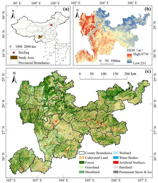
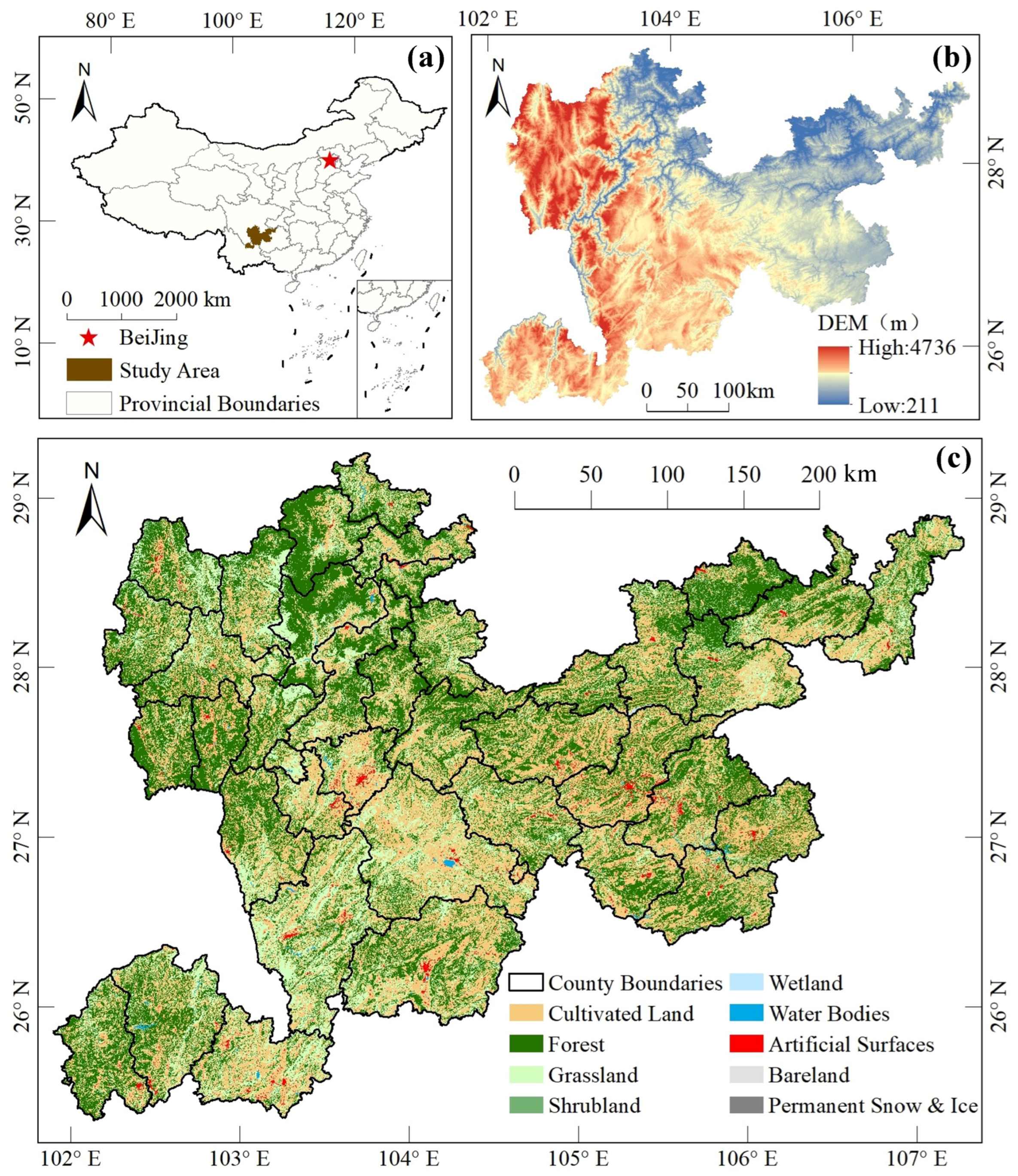
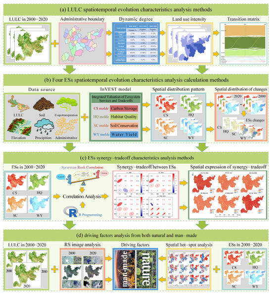
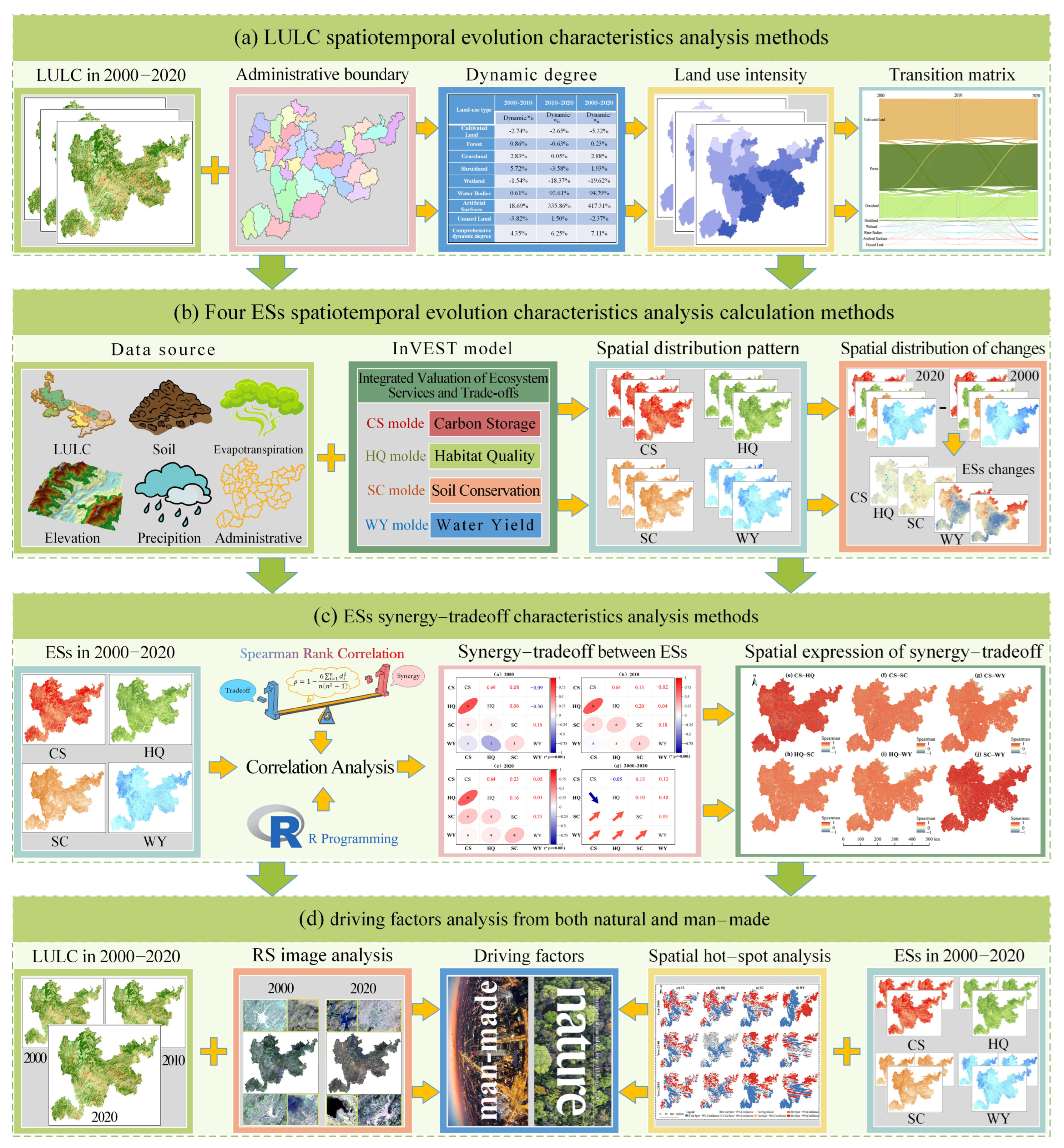
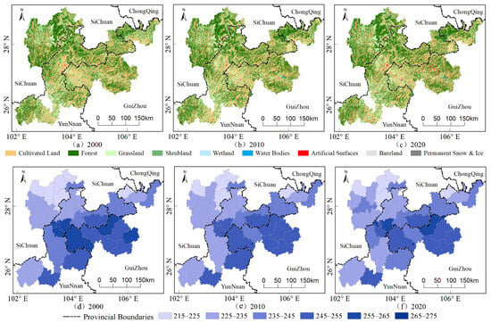
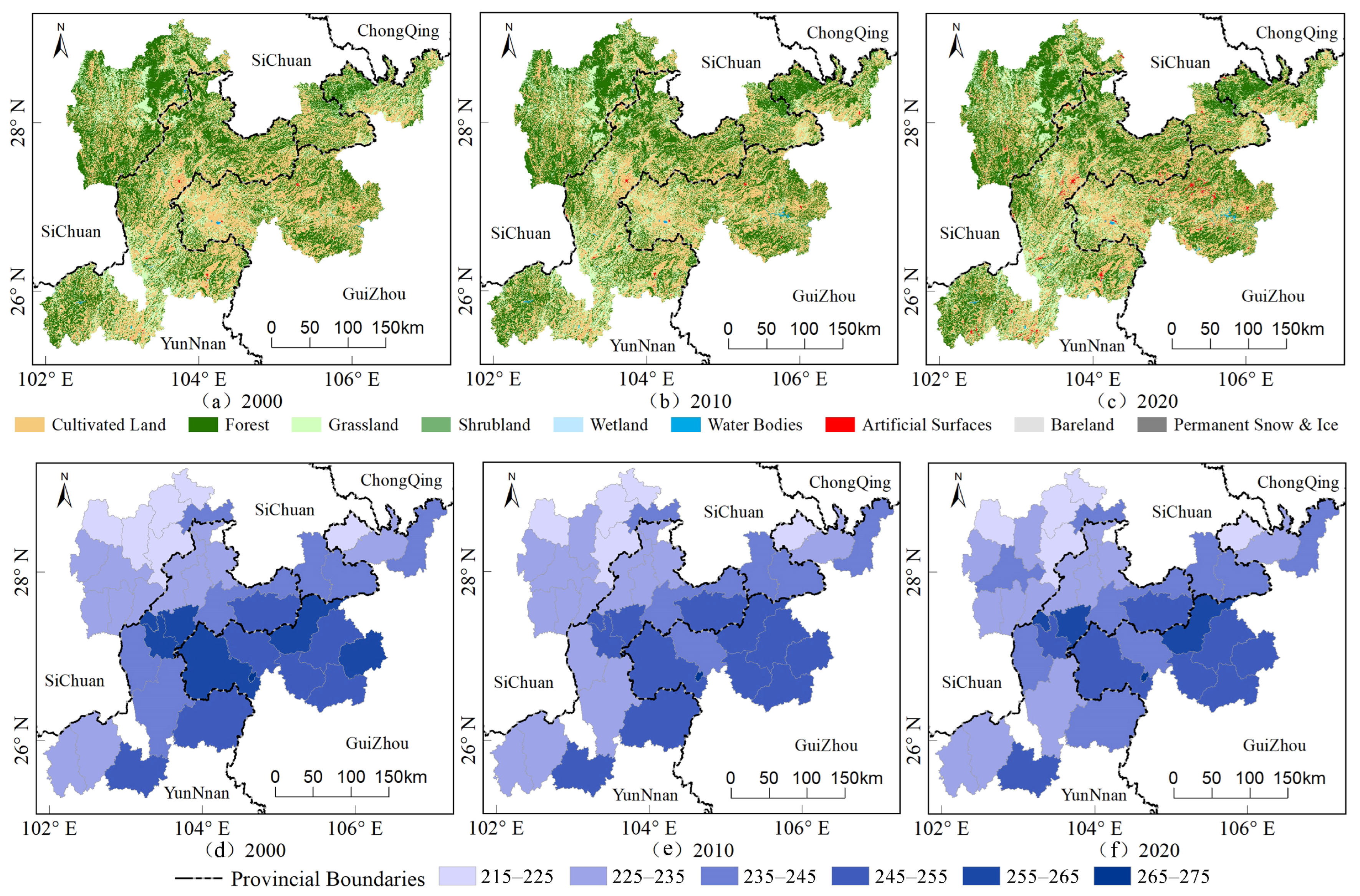
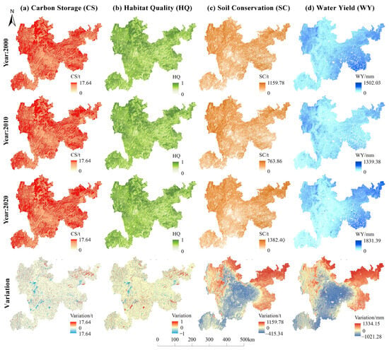
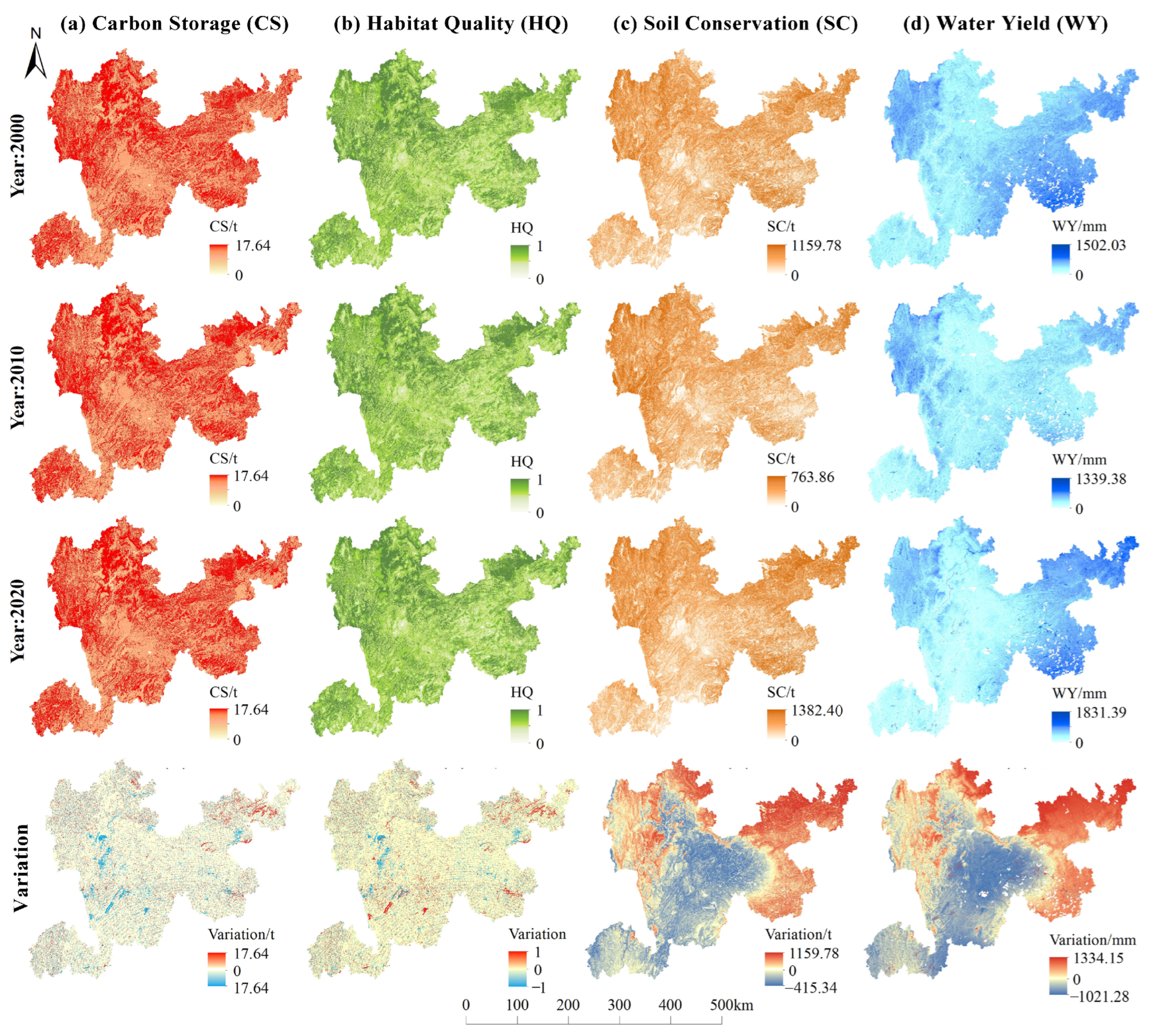
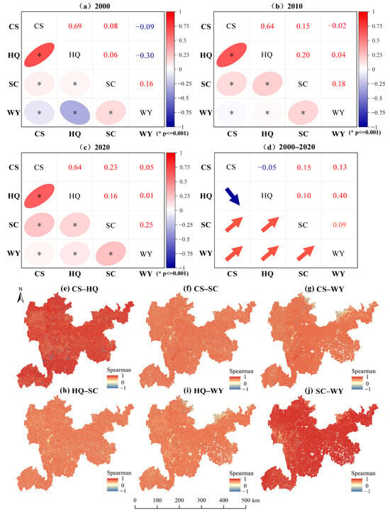
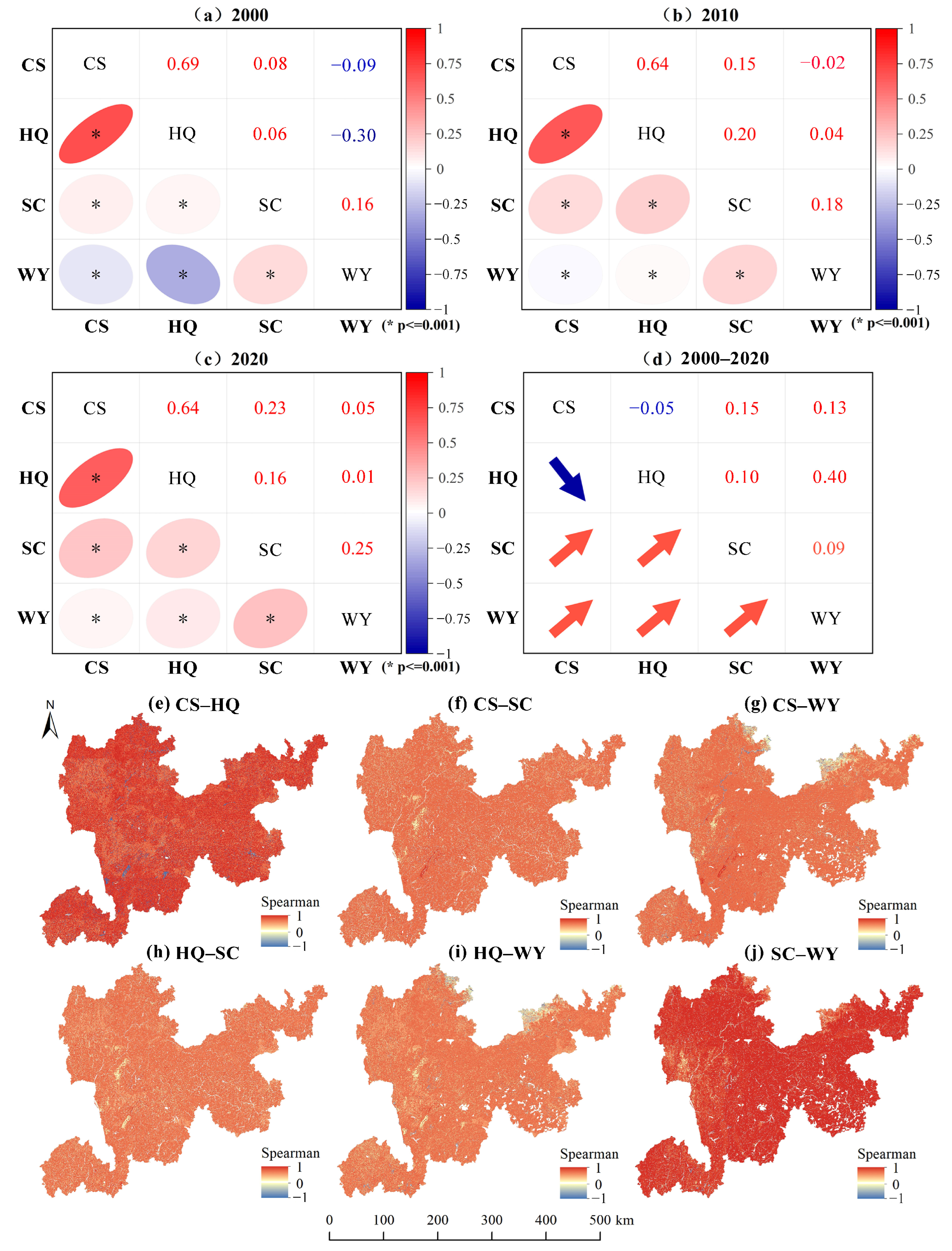
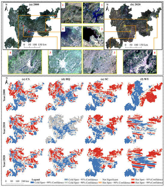
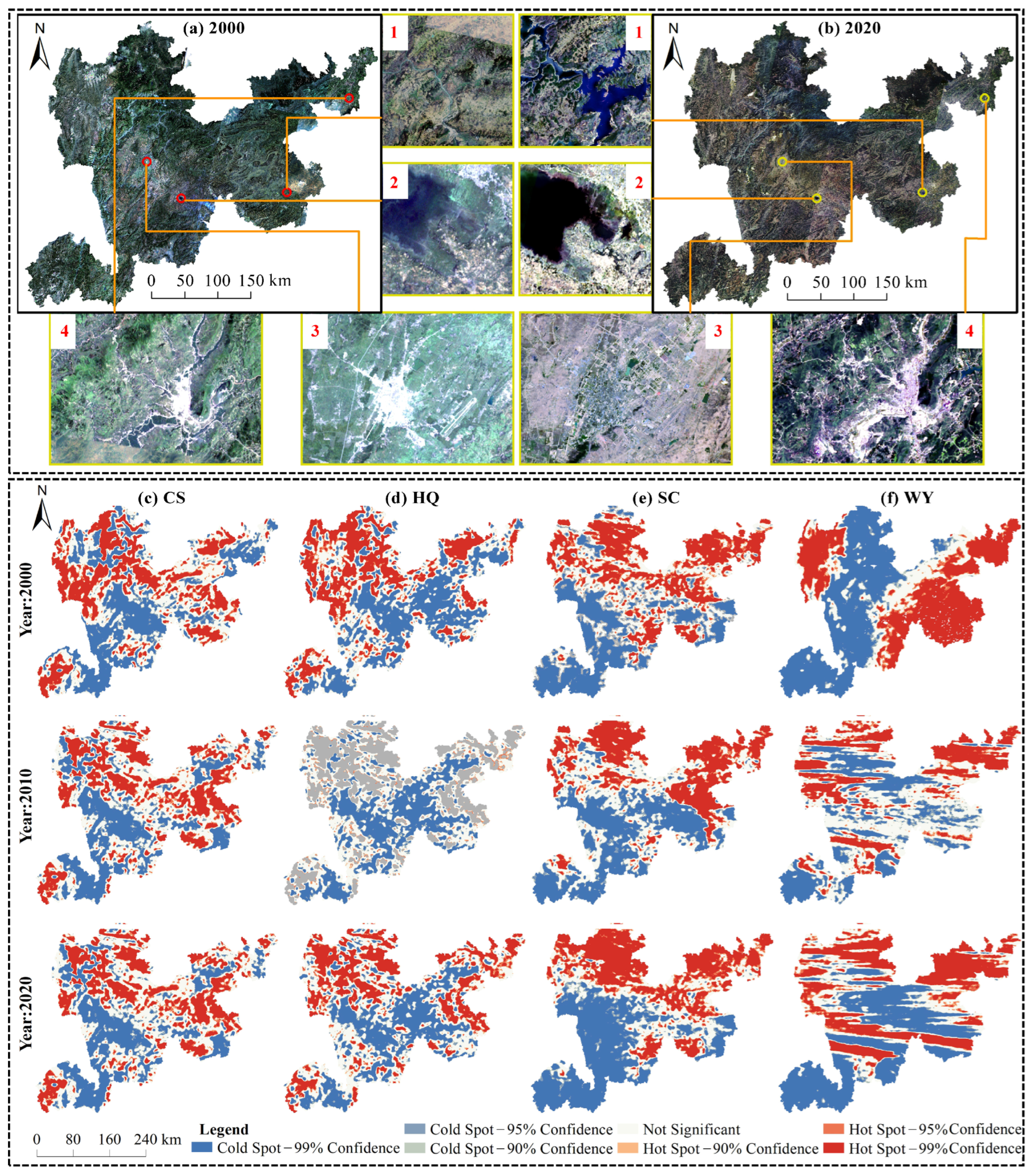

Disclaimer/Publisher’s Note: The statements, opinions and data contained in all publications are solely those of the individual author(s) and contributor(s) and not of MDPI and/or the editor(s). MDPI and/or the editor(s) disclaim responsibility for any injury to people or property resulting from any ideas, methods, instructions or products referred to in the content. |
© 2026 by the authors. Licensee MDPI, Basel, Switzerland. This article is an open access article distributed under the terms and conditions of the Creative Commons Attribution (CC BY) license.