Article

Administrative Fragmentation Distorts Ecological Networks: Mechanisms, Scale Effects, and Optimization Paths


1
College of Ecology and Environment, Chengdu University of Technology, Chengdu 610059, China
2
Yunnan South Geotechnical Engineering Co., Ltd., Dali 671000, China
*
Author to whom correspondence should be addressed.
Forests 2026, 17(5), 611; https://doi.org/10.3390/f17050611
Submission received: 23 March 2026 / Revised: 26 April 2026 / Accepted: 14 May 2026 / Published: 18 May 2026
(This article belongs to the Section Forest Ecology and Management)

Abstract

Administrative fragmentation, whereby political boundaries are used as analytical extents, can disrupt ecological flows and weaken ecological network planning by creating a mismatch between governance units and ecological processes. However, the pathways through which such fragmentation alters network structure and function remain insufficiently quantified. This study quantifies these effects and identifies the landscape conditions that shape the effectiveness of cross-boundary integration. Using a multi-scale buffer experiment (1–32 km) across 30 representative counties in China, we constructed ecological networks based on Morphological Spatial Pattern Analysis and on the minimum cumulative resistance model. Results show that relaxing administrative boundaries reduced structural distortions and lowered total ecological flow cost, indicating that fragmentation increases connectivity costs. Mechanistically, reducing redundant internal links and forced detours improved network efficiency mainly by shortening corridors and lowering flow costs, whereas mean corridor resistance changed little. This suggests that functional degradation is driven primarily by topological disruption rather than by declines in corridor quality. The benefits of cross-boundary integration were greater in counties with regular shapes, high grassland cover, humid climates, and rugged terrain, but weaker under strong human pressure and warmer temperatures. Improvements leveled off beyond 32 km, suggesting a 32 km buffer (study-specific) for integration and supporting context-specific strategies for ecological network planning.

1. Introduction

Landscape fragmentation constitutes a principal driver of global biodiversity loss and ecosystem degradation [1,2,3,4]. Amidst intensifying land-use change and rapid urbanization, natural habitats are increasingly dissected by roads, croplands, and built-up areas (i.e., impervious surfaces) into isolated patches, thereby severely disrupting ecological processes such as species movement and material flows [2]. In this context, the construction of ecological networks is increasingly recognized as a critical spatial strategy for maintaining regional ecological security, enhancing landscape connectivity, and fostering human–nature coexistence [5,6]. By identifying core ecological sources and restoring or protecting potential connecting corridors, ecological networks not only bolster ecosystem resilience to climate change and anthropogenic disturbances [7,8,9] but also provide a scientific blueprint for regional ecological infrastructure planning [10,11]. Consequently, the ecological network concept has been deeply integrated into major conservation policy frameworks, including the Convention on Biological Diversity’s Global Biodiversity Framework [12] and the Ecological Conservation Redline in China [13]. However, the practical implementation of ecological networks faces significant methodological challenges [14,15,16,17]. A key yet often overlooked constraint concerns the spatial delineation of the analysis unit—specifically, overreliance on administrative boundaries—which increasingly undermines their ecological effectiveness [10,15,16,17,18,19].
Contemporary ecological network construction generally adheres to a standardized workflow encompassing ecological source identification, resistance surface modeling, and corridor extraction, with Morphological Spatial Pattern Analysis (MSPA) and the Minimum Cumulative Resistance (MCR) model serving as the predominant technical combination [20,21]. Although the spatial extent of analysis demonstrably and substantially influences the modeling of ecological processes, a persistent misconception in practice equates administrative boundaries with ecologically meaningful spatial units, despite their frequent mismatch with the continuity of actual ecological processes [22]. Such an approach fundamentally disregards the inherent continuity and cross-boundary nature of ecosystem processes [18,22,23,24]. We define “administrative fragmentation” as a methodological limitation whereby the rigid adoption of a single administrative unit as the analytical boundary artificially severs cross-jurisdictional ecological flows and landscape connectivity, thereby systematically underestimating regional connectivity [23,25] (Figure 1). Administrative fragmentation represents a specific manifestation of scale mismatch, wherein management actions fail to align with the ecosystems they affect [18,19,25,26].
Administrative fragmentation represents a manifestation of institutional scale mismatch in global ecological governance rather than merely a technical constraint [16,19,23,27]. This phenomenon reflects the fundamental incongruence between the spatial scales of ecological processes (e.g., species dispersal, hydrological cycles, and material exchange) and administrative jurisdictions, engendering the pervasive dilemma wherein ecological systems operate without boundaries whereas management actions remain bounded [18,28]. Such an administrative-centric analytical paradigm not only generates severe misalignment with the actual spatial scales of ecological processes [23,24] but also jeopardizes conservation investment efficiency through the systematic neglect of critical ecological subsidies from adjacent regions, including cross-boundary source habitats and connecting corridors [10,11,29]. Although previous studies have acknowledged the potential interference of administrative boundaries with ecological network integrity (e.g., [10,30]), a systematic understanding of the pathways, quantitative characteristics, scale effects, and context-dependent mitigation strategies of these distortions remains lacking. In particular, neither the mechanisms linking structural distortions (e.g., missing corridors, detours, redundancy) to functional degradation (e.g., increased ecological flow costs) (Figure 1) nor the role of county-specific background characteristics (e.g., topography, climate, land use) in shaping cross-boundary integration effectiveness have been clarified [31,32]. Furthermore, the policy costs associated with such fragmentation—including misallocated conservation expenditures and unmet biodiversity targets—have received insufficient emphasis [33]. Consequently, scientifically incorporating cross-boundary information to mitigate administrative fragmentation effects while maintaining management operability and identifying optimization pathways tailored to heterogeneous regional contexts constitute urgent priorities for enhancing the ecological efficacy and practical applicability of ecological network planning [11,28,34].
Administrative fragmentation systematically compromises the structural integrity and functional connectivity of ecological networks through cascading mechanisms that fundamentally conflict with the continuous nature of ecological processes [6,18]. Firstly, source omission represents the most direct consequence of administrative delineation (Figure 1). When ecological source patches span administrative boundaries, portions falling outside the jurisdiction are forcibly excluded, resulting in the underestimation or complete omission of source areas. This misclassification may erroneously designate large, continuous habitats that should function as key nodes as isolated small patches, thereby compromising the network’s core supporting capacity [35,36]. Secondly, administrative constraints force corridor detours (Figure 1). Prohibited from establishing cross-boundary connections, minimum cost path algorithms are restricted to seeking alternative routes within administrative regions, frequently generating corridors that detour along boundaries. Such paths typically traverse high-resistance anthropogenic disturbance areas (e.g., built-up areas, croplands), violating species’ natural migration preferences, and are unlikely to be utilized by dispersing organisms in reality, thereby functioning as spurious linkages [37]. These not only fail to facilitate effective migration but also risk misleading conservation investments [29]. Thirdly, topological distortion of network patterns ensues (Figure 1). On the one hand, strategic corridors connecting key habitats inside and outside the jurisdiction are systematically eliminated, severing the core pathways of cross-boundary ecological flows [22]; on the other hand, when a single continuous ecological patch is divided by administrative lines, numerous short-range, high-resistance “pseudo-connections” are generated between internal sub-units, resulting in redundant internal links [28]. This dual distortion of “external loss and internal redundancy” renders networks built upon administrative boundaries superficially connected while substantially impairing their actual capacity to promote population dispersal, material cycling, and ecosystem service provision [2,38], ultimately resulting in a severe disconnect between structural and functional connectivity.
Addressing the inherent tension between continuous ecological processes and the fragmentation imposed by administrative boundaries necessitates a multi-scale optimization framework grounded in ecological functioning. Such an approach aims to identify “effective integration scales” that enhance landscape connectivity without compromising administrative feasibility [18,39]. Existing studies predominantly rely on structural connectivity indices [21] (e.g., IIC and PC); however, these metrics fail to quantify the operational and management costs of ecological networks, often resulting in a disconnect between planning schemes and conservation practices [38]. Consequently, evaluation indicators must move beyond purely structural descriptions to capture the core function of ecological networks: facilitating efficient, low-cost ecological flows [40]. To this end, we adopt Total Ecological Flow Cost (TEFC) as the core functional indicator. Defined as the sum of minimum cumulative resistance values across all ecological corridors within a region, TEFC quantifies the total “ecological engineering” cost required to maintain landscape connectivity [41]. This metric aligns with cost–benefit principles in conservation planning [29] and directly reflects resource-use efficiency in management decisions [42], thereby bridging the gap between structural connectivity metrics and practical conservation implementation.
Based on this framework, we conduct an empirical study across 30 ecologically representative counties in China, using a multi-scale buffering experiment (1–32 km) to systematically investigate the distortion effects of administrative boundaries and potential optimization pathways. We address four core research questions: (1) Does administrative fragmentation systematically distort network structure (i.e., missing cross-boundary corridors [MCC], detour forcing, and redundant internal links [RIL]) and function (i.e., Total Corridor Length [TCL], mean corridor resistance [MCR], and total ecological flow cost [TEFC])? (2) What is the mechanistic link between structural distortion and functional degradation? (3) How do county-level characteristics (geometry, topography, climate, land use, and human disturbance) modulate network sensitivity to cross-boundary integration (buffer expansion)? (4) How do buffer distance and various background characteristics directly moderate raw structural metrics (e.g., corridor loss, detouring, internal redundancy) and functional metrics (e.g., total length, mean resistance, TEFC) across different contexts?

2. Materials and Methods

2.1. Study Area and Sampling Design

The effectiveness of ecological network construction is highly context-dependent [43]. To systematically investigate how administrative fragmentation distorts ecological networks and how such distortions vary with scale, we employed a stratified sampling strategy to select 30 ecologically and geographically representative counties from China’s 2730 county-level administrative units. We compiled an 11-dimensional attribute matrix encompassing geometric complexity, topographic heterogeneity, climatic conditions, anthropogenic disturbance, and land-use composition. These variables included shape index, elevation difference, mean elevation, annual mean temperature, annual precipitation, Human Footprint Index, impervious surface proportion, forest land proportion, cropland proportion, shrubland proportion, and grassland proportion, derived from circa-2020 datasets (Section S1). Following Z-score standardization, K-means clustering was applied to partition counties into 30 characteristic clusters, with k = 30 determined by the elbow method and silhouette width maximization [44,45]. One county was randomly selected from each cluster, yielding a sample spanning eastern plains, southwestern mountains, northwestern arid zones, and northeastern forest–grassland ecotones (Section S1).
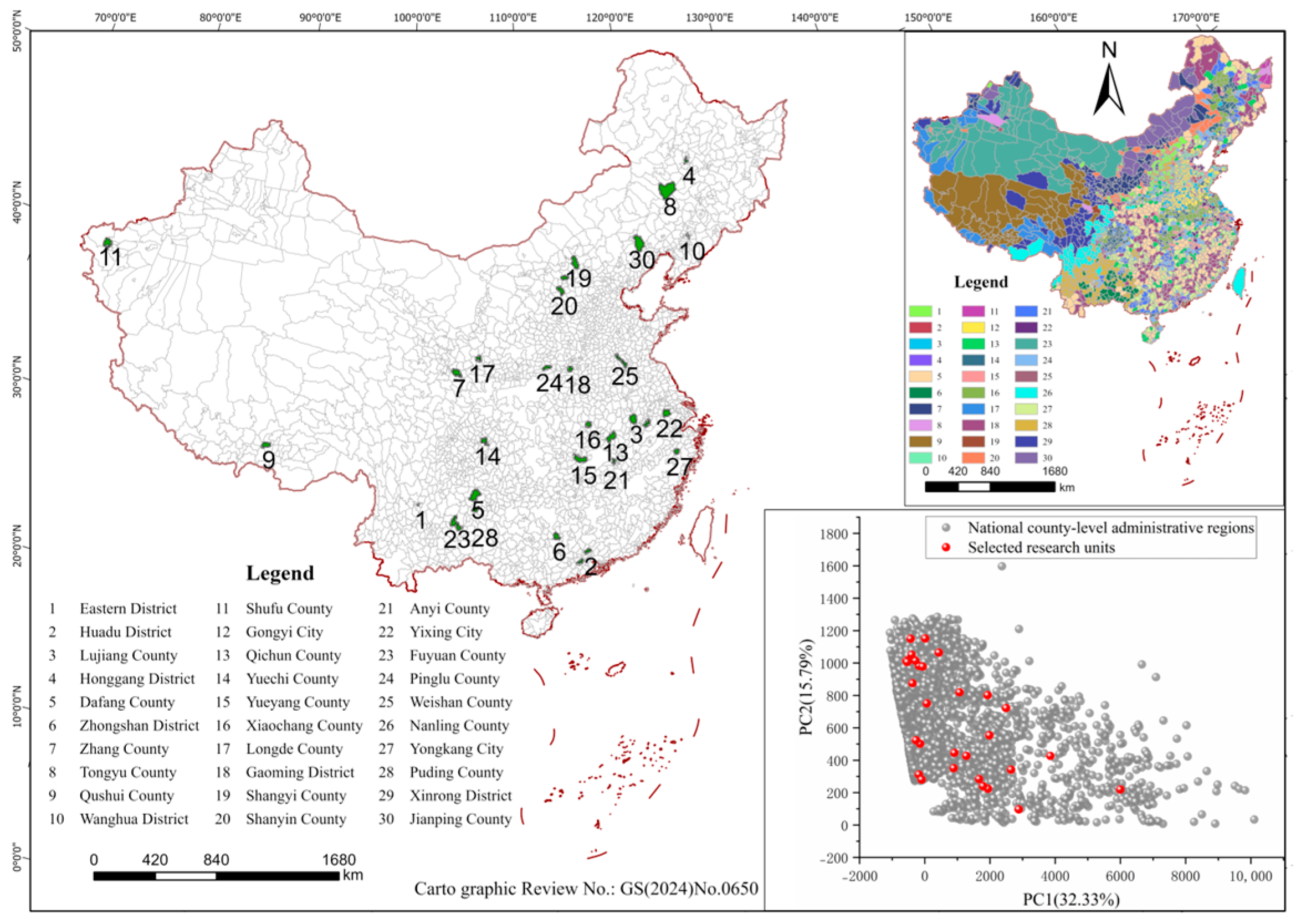
The spatial distribution of the 30 selected counties is shown in Figure 2. These counties are distributed across different ecological and geographic regions of China, including eastern plains, southwestern mountains, northwestern arid zones, northeastern forest–grassland ecotones, and high-elevation plateau areas. The inset cluster map shows the 30 characteristic groups derived from K-means clustering, while the PCA ordination indicates that the selected counties broadly cover the main gradients of county-level background characteristics. Detailed information on county names, area, shape index, elevation, climate, land-use composition, and human disturbance is provided in Table S1.4.

2.2. Multi-Scale Spatial Analysis Unit Construction

We implemented a multi-scale buffer experiment to quantify the distorting effects of administrative boundaries on ecological network structure and function, and to examine how county-level characteristics modulate responsiveness to boundary relaxation. For each county, we generated concentric external buffers at radii of 1, 2, 4, 8, 16, and 32 km around the official administrative boundary, yielding seven nested analysis units. This exponential sequence spans local to regional ecological influence scales while balancing computational efficiency [46].
The outermost buffer of 32 km was adopted based on technical analysis to cover the expected scale of ecological influence and to balance computational feasibility. This value is specific to our study design and is not intended as a general recommendation. This threshold captures the effective dispersal distances of medium-sized terrestrial vertebrates [47,48], aligns with county-level administrative diameters in China (50–80 km), and facilitates coordination with municipal planning frameworks [49]. Furthermore, this threshold represents a connectivity saturation point beyond which marginal gains decline precipitously [50,51], with pilot analyses confirming <5% equivalent connectivity improvement beyond 32 km.
All network modeling procedures—including ecological source identification and corridor extraction—were conducted independently within each buffer extent, whereas evaluation metrics were calculated strictly within original administrative boundaries to ensure cross-scale comparability [52].
The methodological workflow of this study is summarized in Figure 3, encompassing county selection, multi-scale buffer construction, ecological network modeling (source identification, resistance surface construction, and corridor extraction), metric calculation (structural: MCC, DFC, RIL; functional: TCL, MCR, TEFC), and statistical analyses (slope analysis, SEM, MLR, LMM).

2.3. Ecological Network Construction

We constructed ecological networks for each county and its multi-scale buffer extents using a standard three-stage workflow comprising ecological source identification, resistance surface modeling, and corridor extraction [53]. All spatial analyses were conducted in ArcGIS 10.2 using a 30 m raster resolution. This resolution was selected for three reasons. First, it is consistent with the native or widely used standard resolution of the major land-use and environmental datasets employed in this study, thereby minimizing uncertainty introduced by repeated resampling. Second, 30 m provides sufficient spatial detail to capture county-scale landscape heterogeneity and corridor structure while remaining computationally feasible for repeated ecological network modeling across 30 counties and seven nested buffer scenarios. Third, using a uniform 30 m grid ensured full comparability among ecological source identification, resistance surface construction, corridor extraction, and subsequent metric calculation.

2.3.1. Ecological Source Identification

Ecological sources were identified using Morphological Spatial Pattern Analysis (MSPA) implemented in Guidos Toolbox v2.2 [21]. This morphological image processing method avoids percolation biases and window-bound limitations associated with traditional convolution approaches, thereby enhancing pixel-level precision. Forest, grassland, shrubland, and wetland were classified as ecological foreground, whereas cropland, impervious surface, water, and bare land were treated as background [49,52]. Only MSPA core patches ≥ 1 km2—consistent with China’s ecological redline standards and viable population thresholds [49,54]—were retained and converted to centroid points to serve as network nodes.

2.3.2. Resistance Surface Construction

The ecological resistance surface was developed by integrating land use, slope, elevation, and the Human Footprint Index via Spatial Principal Component Analysis to derive objective weights (land use: 0.82; Human Footprint: 0.79; slope: 0.65; elevation: 0.58; PC1 explained 68.2% variance, PC2 explained 17.5%) followed by weighted summation. The apparent difference between the weights reported in the Supplementary Materials and the main text reflects different stages of the analysis: the Supplementary Materials show the raw SPCA factor loadings, whereas the main text reports the final standardized weights used to generate the integrated resistance surface for MCR calculations. This categorical matrix approach balances assessment accuracy with practical applicability, providing reliable proxies for patch importance ranking while primarily influencing corridor delineation rather than prioritization outcomes [55] (Section S2).

2.3.3. Ecological Corridor Identification

Potential corridors were extracted using Linkage Mapper v2.0.4 implementing the Minimum Cumulative Resistance model, which quantifies movement difficulty by integrating distance and landscape resistance through cost-weighted path analysis [24,56]. The links corresponding to the lowest 95% of cost distances were retained for analysis, while the top 5% of highest-cost links were excluded. Model parameters, including the normalized cost corridor (NCC) threshold used to delineate potential corridors, are detailed in Section S3. Identification of ecological corridors using the MCR model. This selection ensures that the majority of ecologically relevant pathways are considered while removing extreme-cost connections that are unlikely to be utilized [32]. Ecological corridors were identified using the Minimum Cumulative Resistance (MCR) model implemented through the Linkage Mapper toolbox (v2.0.4) in ArcGIS 10.2. Core ecological sources were defined as centroids of MSPA core patches ≥ 1 km2, and the SPCA-derived integrated resistance surface served as input [21,22].
The Pinchpoint Mapper module was applied to identify potential bottlenecks along the least-cost corridors [6]. Additionally, CircuitScape 5.0 was employed to simulate multiple dispersal pathways and cumulative current flow across the resistance surface [24]. The CircuitScape outputs were overlaid with MCR corridors to highlight redundancy and critical pinch points, ensuring that multiple dispersal pathways were considered.
All structural and functional metrics—Total Corridor Length (TCL), Mean Corridor Resistance, and Total Ecological Flow Cost (TEFC)—were calculated based solely on MCR-defined corridors within each buffer extent [38,41]. CircuitScape results were used to validate corridor redundancy and pinch points but were not directly included in metric calculations (Section S3).

2.4. Evaluation Metric System

We developed a dual-tiered metric system integrating structural metrics (MCC, DFC, RIL) derived from binary habitat maps and functional metrics (TCL, MCR, TEFC) based on resistance-weighted ecological flows to diagnose administrative fragmentation effects and assess multi-scale buffering improvements [43,57]. This approach captures both structural distortions and functional degradation while ensuring comprehensive assessment of habitat availability. All metrics were computed within original administrative boundaries and normalized per 10,000 km2 via area-proportional scaling and landscape shape index (LSI)-based correction to control for area effects and ensure cross-county comparability (Section S4).

2.4.1. Structural Distortion Diagnostics

Structural distortion was quantified using three complementary metrics normalized per 10,000 km2. Missing Cross-boundary Corridors (MCCs) count connections present in buffered scenarios but absent in unbuffered ones, indicating strategic linkages severed by administrative boundaries. Detour Forcing Count (DFC) quantifies corridors forced to circumvent boundaries along higher-resistance edge routes when direct cross-boundary paths are excluded. Redundant Internal Links (RILs) capture spurious connections between sub-patches of single continuous habitats artificially fragmented by administrative delineation [40] (Figure 1).

2.4.2. Functional Optimization Metrics

Functional connectivity was assessed using three resistance-based metrics normalized per 10,000 km2 where applicable. Total Corridor Length (TCL) quantifies the geometric extent of the network. Mean Corridor Resistance (MCR) measures average movement efficiency across all corridors, with lower values indicating reduced impedance. Total Ecological Flow Cost (TEFC) integrates network extent and quality by summing cumulative resistance values, representing the total energetic investment required to maintain connectivity and aligning with cost–benefit optimality in conservation planning [29,41,56]. This functional suite complements structural metrics by linking spatial patterns to ecological processes, avoiding purely descriptive analysis [38] and enabling quantitative identification of optimization thresholds for planning applications.

2.5. Statistical Analysis

We employed a multi-stage analytical framework to examine the impacts of administrative fragmentation on ecological networks, elucidate the structural–functional pathways of distortion, and assess how county-level context modulates the efficacy of cross-boundary integration. All continuous variables, with the exception of buffer distance, were Z-score standardized. Buffer distance was log-transformed to linearize its non-linear relationship with connectivity and to align with scale-dependent ecological process models [24,54].

2.5.1. Slope Analysis of Evaluation Metrics with Respect to Buffer Distance

We quantified county-scale sensitivity to cross-boundary integration by regressing each of the six structural and functional metrics (MCC, DFC, RIL, TCL, MCR, TEFC) against log-transformed buffer distance. The resulting slope coefficients served as standardized indicators of responsiveness to spatial scale expansion [54]. Negative values for MCCslope, DFCslope, RILslope, TCLslope, MCRslope, and TEFCslope indicate stronger positive buffering effects (i.e., greater reductions in distortions and costs). This approach enabled cross-county comparability of network-performance sensitivity and facilitated the identification of counties where administrative fragmentation most severely constrains ecological connectivity.

2.5.2. Structural Equation Modeling (SEM)

We employed SEM to disentangle the causal pathways linking administrative fragmentation to functional degradation. We hypothesized that structural distortions (MCCslope, DFCslope, RILslope) mediate network scale (TCLslope) and quality (MCRslope), thereby driving total ecological flow cost (TEFCslope) [38,40]. The model was fitted via maximum likelihood estimation, with standardized path coefficients quantifying direct and indirect effects. Model fit was assessed using χ2/df, RMSEA, GFI, and SRMR following standard criteria [58].

2.5.3. Multiple Linear Regression Models

We used separate multiple linear regression models to examine how county-level biophysical and anthropogenic characteristics influenced the responsiveness of ecological networks to cross-boundary integration, with the slope of each metric (MCCslope, DFCslope, RILslope, TCLslope, MCRslope, and TEFCslope) as the response variable. Candidate predictors included SHID, ELED, ELEM, TEMP, APRE, HMFT, ISP, FLPR, CLPR, SLPR, and GLPR, together with selected theoretically meaningful two-way interaction terms. All continuous predictors were Z-score standardized. Multicollinearity was evaluated using variance inflation factors (VIF), and variables with VIF ≥ 5 were not included in the same candidate model. Final models were selected using AICc-based stepwise comparison [59], and adjusted R2 was used to assess explanatory power. Table 1 reports the standardized coefficients of the best-fitting model for each slope metric.

2.5.4. Linear Mixed-Effects Models (LMMs)

We used linear mixed-effects models to assess how raw ecological network metrics (MCC, DFC, RIL, TCL, MCR, and TEFC) varied with buffer distance and county-level context across all county–buffer combinations. Fixed effects included log-transformed buffer distance (BUFFER), the same contextual variables used in the regression analysis, and selected theoretically meaningful two-way interaction terms, especially those involving BUFFER. County identity was included as a random intercept to account for repeated observations across the seven buffer scenarios within each county. Continuous predictors were standardized, whereas BUFFER was log-transformed. Because residual spatial autocorrelation was significant (Moran’s I = 0.32, p < 0.01), a spatial lag term was included as an additional fixed effect [60]. Models were fitted using restricted maximum likelihood (REML) with VIF screening (<5) and AICc-based model selection [24]. Table 2 presents the standardized coefficients of the final mixed-effects models.

2.6. GenAI Tool Usage Declaration

During the preparation of this manuscript, GenAI tools, including Doubao v13.2.0, Tencent Yuanbao v2.68.0, and Qianwen v6.9.5.2879, were used for specific tasks under the full supervision, review, and final approval of the authors. Their specific uses are as follows:
  • In the statistical analysis process, R 4.3.0 software was employed, and GenAI was leveraged to optimize the code;
  • GenAI was used to refine the language of the manuscript.
During the preparation of this manuscript, the authors used Doubao, Tencent Yuanbao, and Qianwen (web versions accessed in April 2026) for code optimization assistance and language polishing. The authors reviewed and edited all AI-assisted outputs and take full responsibility for the content of this publication.

3. Results

3.1. Administrative Fragmentation Systematically Distorts Network Structure and Function

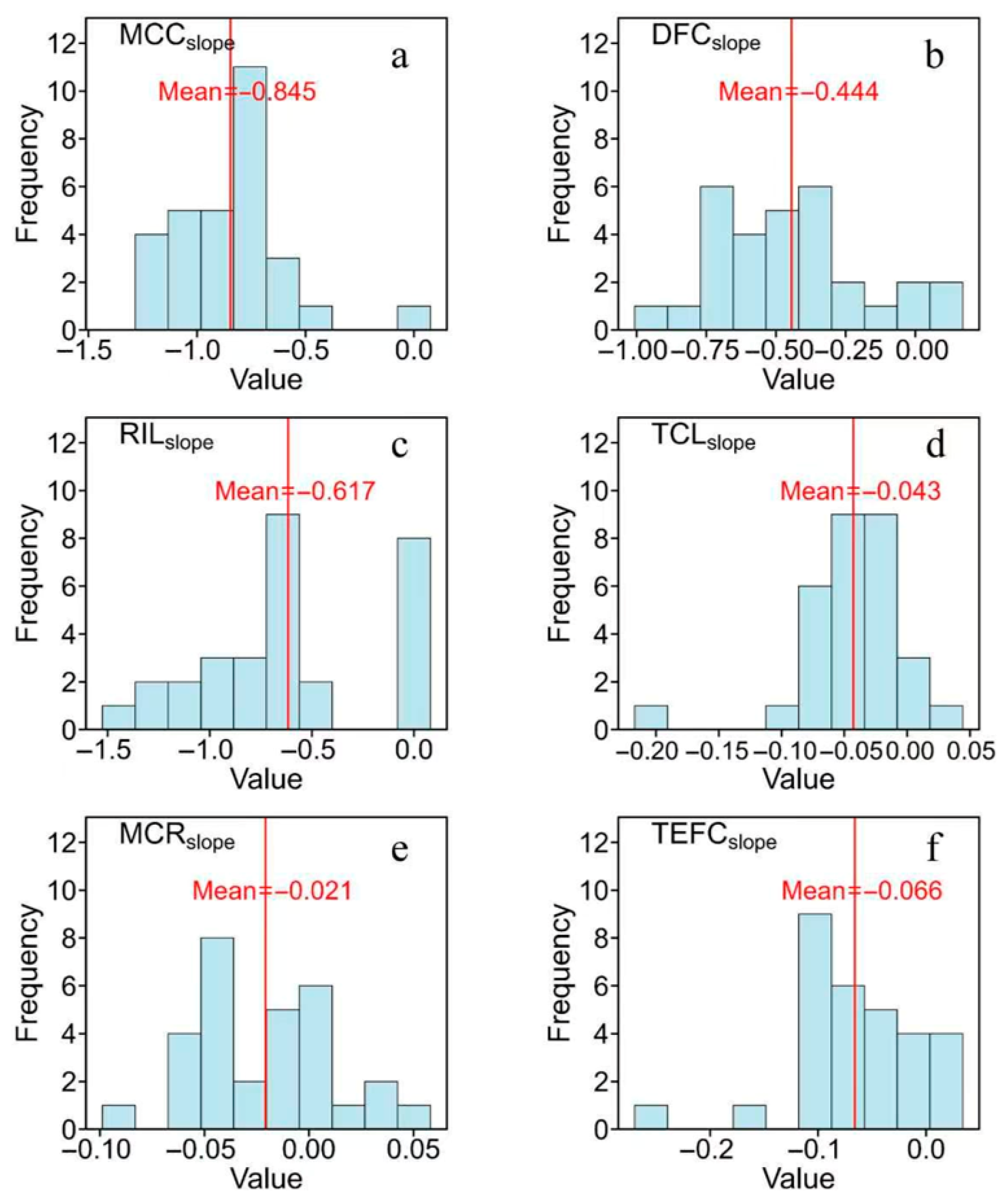
Across the 30 sample counties, administrative fragmentation was associated with systematic, scale-dependent disruptions in ecological network structure and selected aspects of network function (Figure 4). Frequency distributions of metric-specific response slopes (i.e., rates of change with respect to log-transformed buffer distance) revealed that five of the six indicators exhibited significantly negative slopes (all p < 0.001).
Structural distortion metrics demonstrated the strongest sensitivity to boundary relaxation. Missing Cross-boundary Corridors (MCCs) exhibited the steepest decline with buffer expansion (mean slope = −0.845, 95% CI: −1.021 to −0.668), followed sequentially by Redundant Internal Links (RILs; mean slope = −0.617, 95% CI: −0.783 to −0.451) and Detour Forcing Count (DFC; mean slope = −0.444, 95% CI: −0.592 to −0.296) (Figure 4a–c).
Functional metrics corroborated these structural degradation patterns. Total Corridor Length (TCL) declined significantly with increasing buffer width (mean slope = −0.043, 95% CI: −0.068 to −0.018; Figure 4d), whereas Total Ecological Flow Cost (TEFC) exhibited the second-steepest response (mean slope = −0.066, 95% CI: −0.091 to −0.041; Figure 4f). Mean Corridor Resistance (MCR), derived using the Minimum Cumulative Resistance model, showed no significant improvement with buffer expansion (mean slope = −0.021, 95% CI: −0.053 to 0.011, p = 0.229; Figure 4e). Here, MCR is the indicator of average corridor resistance, and the MCR model is the method used to calculate it.

3.2. Structural Distortions Drive Functional Degradation Through Cascading Pathways

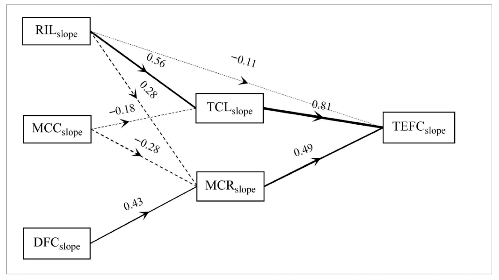
Structural equation modeling (SEM) confirmed the hypothesized mediation pathways linking structural distortion mitigation to functional cost reduction (Figure 5). The model exhibited excellent fit (χ2/df = 1.82, CFI = 0.94, RMSEA = 0.052, SRMR = 0.048). Reductions in redundant internal links (RILslope) significantly predicted declines in total corridor length (TCLslope; standardized β = 0.56, p < 0.001). Both RILslope (β = 0.28, p < 0.05) and reductions in detour forcing (DFCslope; β = 0.43, p < 0.001) significantly predicted improvements in mean corridor resistance (MCRslope). By contrast, missing cross-boundary corridors (MCCslope) showed no significant direct effects on either TCLslope (β = −0.18, p > 0.05) or MCRslope (β = −0.28, p > 0.05) (dashed lines in Figure 5). Network scale reduction (TCLslope) and efficiency improvement (MCRslope) both significantly predicted decreases in total ecological flow cost (TEFCslope), with standardized path coefficients of 0.81 (p < 0.001) and 0.49 (p < 0.001), respectively. The direct path from RILslope to TEFCslope was non-significant (β = −0.11, p > 0.05).

3.3. Context-Dependent Sensitivity of Network Responses to Cross-Boundary Integration

Multiple linear regression models revealed that county-level biophysical and anthropogenic characteristics substantially modulated network responsiveness to buffer expansion (Table 1). As all slope-dependent variables were negative (indicating improvement with buffer expansion), positive regression coefficients denote characteristics that attenuated sensitivity (i.e., slower improvement), whereas negative coefficients denote characteristics that amplified sensitivity (i.e., faster improvement).
Sensitivity of structural distortion to buffer expansion varied significantly across contextual gradients. Counties with higher Shape Index (SHID) exhibited attenuated sensitivity in Missing Cross-boundary Corridors (MCCs; β = 0.148, p < 0.001). Similarly, higher Annual Mean Temperature (TEMP) attenuated MCC sensitivity (β = 0.224, p < 0.001). Conversely, higher Annual Precipitation (APRE) amplified MCC sensitivity (β = −0.177, p < 0.01).
Internal redundancy reduction (RILslope) was significantly predicted by multiple land-use and topographic variables. Higher Forest Land Proportion (FLPR; β = −0.340, p < 0.001), Impervious Surface Proportion (ISP; β = −0.471, p < 0.01), and Elevation Difference (ELED; β = −0.257, p < 0.05) all amplified RIL sensitivity. Human Footprint Index (HMFT) attenuated RIL sensitivity (β = 0.321, p < 0.01). No significant predictors emerged for Detour Forcing Count slope (DFCslope; adjusted R2 = 0.273).
Functional cost sensitivity (TEFCslope) was primarily driven by interaction effects. The SHID × GLPR interaction significantly amplified TEFC sensitivity (β = −0.041, p < 0.01). Elevation Difference amplified Total Corridor Length reduction (TCLslope; β = −0.022, p < 0.05). No single county characteristic or interaction term significantly predicted Mean Corridor Resistance slope (MCRslope; all p > 0.05).

3.4. Buffer Distance and Landscape Characteristics Jointly Shape Network Dynamics

Linear mixed-effects models (LMMs) showed that buffer expansion significantly reduced all six ecological network metrics (all p < 0.001; Table 2), indicating that relaxing administrative boundaries consistently alleviated structural distortion and functional cost. Because the dependent variables were raw metric values, negative coefficients for BUFFER indicate that larger buffer distances were associated with lower levels of network disruption or movement cost. The fixed effects explained a substantial proportion of the variance across models, with marginal R2 values ranging from 0.38 for DFC to 0.73 for TCL.
For the structural indicators, buffer distance had strong negative effects on MCC, DFC, and RIL, confirming that boundary relaxation reduced missing cross-boundary corridors, detour forcing, and redundant internal links. However, these improvements were not spatially uniform. The positive BUFFER × SHID effects for MCC and DFC indicate that, in counties with more complex landscape shapes, the beneficial effect of buffer expansion was weaker, suggesting that irregular landscape configuration constrains the extent to which boundary relaxation can restore structural connectivity. By contrast, the negative BUFFER × FLPR effect on RIL suggests that higher forest cover strengthened the reduction in redundant internal links with buffer expansion, whereas the positive BUFFER × TEMP effect indicates that this improvement was attenuated in warmer counties.
Among the functional metrics, TCL declined significantly with increasing buffer distance, and its negative associations with elevation and temperature suggest that corridor extent was generally lower in higher and warmer counties. MCR also decreased with buffer expansion, but its response was comparatively modest. Elevation and temperature both had positive main effects on MCR, indicating generally higher corridor resistance in high-elevation and warmer counties, whereas the negative BUFFER × ELEM interaction suggests that buffer expansion reduced MCR more strongly in high-elevation settings, although this reduction remained constrained by persistent topographic resistance.
TEFC showed a significant negative response to buffer distance, indicating that ecological flow became less costly as administrative boundaries were relaxed. Because TEFC represents the cumulative cost of ecological movement across the network, lower TEFC values can be interpreted as improved ecological connectivity and more efficient movement pathways. Several landscape characteristics further modified this pattern. In particular, GLPR had the strongest negative main effect on TEFC (β = −1.782, p < 0.001), highlighting grassland proportion as the most influential predictor of reduced ecological flow cost. The negative SHID × GLPR and TEMP × GLPR interactions suggest that grassland-dominated landscapes further reduced TEFC under more complex landscape structure and warmer climatic conditions. Likewise, the negative TEMP × HMFT interaction indicates that the relationship between human footprint and ecological flow cost was also conditioned by temperature. Taken together, these results suggest that the connectivity benefits of boundary relaxation are strongest where grassland availability is high and where landscape context reinforces reductions in cumulative movement cost.

4. Discussion

Multi-scale buffer experiments conducted across 30 ecologically representative Chinese counties provide the first regional-scale empirical quantification of how administrative fragmentation—an institutional-scale mismatch—systematically distorts ecological network structure and function. By disentangling causal pathways from structural distortion to functional degradation and identifying context-dependent mitigation strategies, this study advances theoretical understanding of scale mismatches in social–ecological systems [18,19], while offering actionable guidance for cross-boundary conservation planning within fragmented governance landscapes.

4.1. Mechanisms of Administrative Fragmentation: From Structural Distortion to Functional Degradation

Our results indicate that administrative boundaries can distort ecological networks through three recurrent structural effects: loss of cross-boundary linkages, detour forcing, and artificial internal redundancy. With increasing buffer distance, Missing Cross-boundary Corridors (MCCs), Detour Forcing Count (DFC), and Redundant Internal Links (RILs) all declined significantly, indicating that many “missing” or inefficient configurations in county-based networks were partly produced by the analytical truncation of ecological processes at administrative borders. This pattern supports the broader argument that ecological processes and management units often operate at mismatched spatial scales [18,19,23].
These structural distortions also had functional consequences. Total Corridor Length (TCL) and Total Ecological Flow Cost (TEFC) declined with buffer expansion, showing that cross-boundary integration can reduce both the geometric extent and the cumulative resistance cost of the network. In practical terms, networks defined strictly within administrative borders required longer or less efficient routing to maintain internal connectivity. By contrast, boundary relaxation allowed more direct configurations and lower overall movement cost. This is consistent with previous work showing that cross-jurisdictional ecological connections can improve the efficiency and robustness of ecological security patterns [10,22,61].
The response of Mean Corridor Resistance (MCR) was more nuanced. In the county-level slope analysis, the average decline in MCR with buffer expansion was not significant, indicating that improvements in corridor quality were weaker and less consistent than improvements in network topology. At the same time, the mixed-effects models detected a modest overall decline in raw MCR across all county–buffer combinations. Taken together, these results suggest that relaxing administrative boundaries can improve corridor resistance in some contexts [62], but that the dominant effect of administrative fragmentation lies in how boundaries reorganize the network—by removing strategic links, forcing detours, and generating redundant internal paths—rather than in uniformly degrading the intrinsic quality of individual corridors [24,38].

4.2. Unpacking the Chain Mechanism: From Structural Repair to Functional Enhancement

The structural equation model helps explain how these structural changes translate into lower ecological flow cost. Specifically, reductions in redundant internal links were strongly associated with shorter total corridor length, while reductions in both redundant internal links and detour forcing were associated with lower mean corridor resistance. Total corridor length and mean corridor resistance then jointly contributed to lower TEFC. This pathway indicates that the functional benefit of boundary relaxation did not arise from a single mechanism; instead, it emerged through the combined effects of network shortening and modest resistance improvement.
One important result is that MCC did not show a significant direct effect on either TCL or MCR in the SEM. This should not be interpreted as meaning that missing cross-boundary corridors are unimportant. Rather, it suggests that, in our dataset, the measurable reduction in ecological flow cost was more immediately associated with correcting inefficient internal topology—especially redundancy and detour forcing—than with restoring missing cross-boundary links alone. Missing corridors may still matter indirectly, or their effects may depend more strongly on local landscape context than can be captured by direct paths in the SEM [34,42].
The stronger role of RIL in the pathway to lower TEFC is particularly informative. Administrative fragmentation can split continuous habitats into multiple internal sub-units and thereby create spurious short-range links that increase network complexity without improving movement efficiency. When these artificial internal redundancies are reduced, the network becomes structurally simpler and functionally cheaper to maintain. Likewise, reducing detour forcing helps replace boundary-constrained routes with more direct pathways. Together, these results suggest that the benefit of cross-boundary integration is not simply the addition of more corridors, but the reorganization of the network into a more coherent and less costly configuration.

4.3. Differentiated Optimization Strategies Based on Background Characteristics

The responsiveness of ecological networks to cross-boundary integration is profoundly regulated by county-level biophysical and anthropogenic characteristics, necessitating context-specific rather than standardized optimization strategies. Multiple regression and mixed-effects models revealed that geometric, climatic, and land-use factors govern the magnitude and mechanisms of buffer expansion benefits through both main and interaction effects.
Geometric and climatic context: Counties with regular boundaries exhibited attenuated sensitivity to Missing Cross-boundary Corridors (MCCs) because compact geometry inherently minimizes cross-boundary habitat continuity. This geometric constraint, combined with the finding that the majority of Chinese counties exhibit intermediate boundary complexity, suggests that most jurisdictions face moderate rather than severe geometric barriers to cross-boundary integration. The positive moderating effect of temperature on MCC slope indicates that, all else being equal, warmer regions exhibit weaker responses in cross-boundary corridor restoration to buffer expansion. This phenomenon can be attributed to higher metabolic costs and constrained dispersal behaviors of species under thermally stressful environments, which limits the actual enhancement of cross-boundary habitat connectivity [35,63]. Conversely, humid climates amplified MCC sensitivity, suggesting that precipitation-mediated productivity supports denser habitat networks where cross-boundary connectivity yields stronger functional gains.
Land-use composition and redundancy dynamics: The amplified sensitivity to Redundant Internal Links (RILs) within forested, urbanized, and rugged terrains reveals distinct mechanisms of internal network distortion. In forested landscapes, administrative boundaries frequently bisect continuous woodland patches, generating abundant redundant internal links that can be eliminated through cross-boundary recognition. This pattern corroborates findings that forested matrices facilitate responsive internal network rationalization when boundary constraints are relaxed [64]. Urbanized counties exhibit similar patterns because impervious surfaces force corridor detours, creating artificial internal connections among fragmented habitat remnants. Rugged terrain amplifies RIL sensitivity because topographic complexity concentrates habitats along elevational gradients, rendering administrative boundaries more likely to intersect continuous habitat patches. However, the attenuating effect of human footprint intensity suggests that intensive anthropogenic activity fundamentally alters network topology—where human disturbance is pervasive, habitat patches are already functionally isolated, and cross-boundary integration cannot restore connectivity that has been eliminated rather than merely obscured by administrative delineation.
Interaction-driven functional optimization: The dominance of interaction effects over main effects in predicting Total Ecological Flow Cost (TEFC) sensitivity indicates that optimal integration strategies require simultaneous consideration of multiple contextual dimensions. The interaction between Shape Index (SHID) and Grassland Proportion (GLPR) demonstrates that regular boundaries combined with extensive grasslands achieve disproportionate efficiency gains—likely because grassland matrices facilitate low-resistance movement, and regular geometries enable complete capture of cross-boundary flows within modest buffer distances. The combination of regular county boundaries and extensive grassland cover represents a particularly favorable context for mitigating administrative fragmentation. The interaction between Temperature (TEMP) and Grassland Proportion (GLPR) indicates that warm-climate grasslands remain functionally connected despite thermal stress, possibly because these landscapes support continuous herbaceous cover that facilitates species movement. Conversely, the interaction between Temperature (TEMP) and Human Footprint (HMFT) attenuates cost improvements, highlighting that intensive human activity in warm climates creates compounding barriers that buffer expansion alone cannot overcome, necessitating complementary in situ conservation interventions.
Elevation and temperature modulation: Linear mixed-effects models corroborated and extended these sensitivity patterns. While buffer expansion universally improves network performance, the magnitude of improvement varies systematically with landscape context. High-elevation counties achieve more rapid network rationalization because topographic heterogeneity concentrates habitat distributions, rendering corridor networks more responsive to boundary relaxation. However, elevation had a positive main effect on MCR, indicating higher average corridor resistance in high-elevation counties. The negative buffer × elevation interaction further suggests that increasing buffer distance reduced MCR more strongly in these counties. Nevertheless, this reduction was not sufficient to overcome the persistent resistance imposed by topography. This persistent resistance underscores the need to integrate multi-species connectivity requirements, as topographic complexity often disrupts habitat continuity for multiple taxa simultaneously [65]. Cool counties achieve more rapid reductions in Total Corridor Length (TCL), whereas warm counties exhibit attenuated improvements in Mean Corridor Resistance (MCR), reflecting metabolic and dispersal constraints that limit functional returns from corridor restoration in thermally stressful environments [66].
Context-independence of corridor quality: The absence of significant predictors for MCR sensitivity corroborates the earlier finding that mean corridor resistance is largely context-independent, responding minimally to either buffer expansion or county-level characteristics. This reinforces the conclusion that functional degradation from administrative fragmentation stems primarily from disrupted connection patterns—as captured by TCL and TEFC—rather than from declines in individual corridor quality. This dissociation between significant TEFC decline and non-significant MCR response highlights that administrative fragmentation degrades network function through topological disruption rather than individual corridor quality decline, aligning with the distinction between structural and functional connectivity [38].
Predictive resource allocation and governance integration: The observed differences in TEFC and structural responses suggest that the benefits of cross-boundary integration are not uniform across counties. Counties with amplifying interaction profiles—such as high grassland cover under relatively regular boundary conditions—may benefit more from broader integration, whereas counties with attenuating profiles (e.g., strong human footprint under warm conditions) may require boundary relaxation to be combined with local habitat restoration or resistance reduction measures. These patterns indicate that conservation planning should match the degree of cross-boundary integration to local landscape context. Because practical implementation also depends on governance capacity, historical cooperation, and shared environmental goals, future planning should integrate ecological and institutional considerations [67].

4.4. Towards an Ecological Process-Based Paradigm for Cross-Administrative Network Planning

These findings support planning approaches based on ecological processes rather than administrative units. Modeling networks beyond boundaries but evaluating within management units captures critical sources and pathways while remaining operationally feasible [22,23].
Context-specific strategies are essential: integration should match local ecological and anthropogenic conditions, combining technical optimization with institutional coordination [27,68]. In this study, the 32 km buffer was used as a study-specific technical analysis scale for cross-boundary integration; larger extents may be required for broader ecological processes [16,46].
Total Ecological Flow Cost (TEFC) quantifies the cumulative cost required to maintain ecological connectivity across the network [32,38,41]. While decreases in TEFC generally reflect more efficient connectivity due to reductions in redundant internal links and detour forcing, TEFC is influenced by overall network topology rather than the quality of individual corridors. Consequently, a low TEFC value does not necessarily indicate fully sufficient connectivity in highly fragmented landscapes; some counties may still exhibit structural discontinuities that limit actual species movement or material flow.
TEFC should be interpreted in combination with structural metrics (e.g., MCC, DFC, RIL) to fully assess network integrity. Analysts and planners should recognize that TEFC reductions primarily signal improvements in topological efficiency rather than absolute connectivity sufficiency. This clarification establishes the interpretive boundaries of TEFC and emphasizes the need for complementary structural indicators when evaluating ecological networks.
Adopting ecological processes as the central organizing principle enables adaptive, context-specific conservation planning, balancing functional benefits and administrative constraints and aligns with global connectivity conservation frameworks [34,69].

4.5. Limitations and Future Prospects

This study is subject to three main limitations. First, the resistance surface adopted herein assumes species-neutral movement patterns; future research should incorporate empirical dispersal data to test the generalizability of our findings across different taxonomic groups [70]. Second, optimal scales of integration likely vary with organism mobility; future studies could utilize species-specific dispersal kernels to determine adaptive thresholds [46]. Third, the treatment of administrative boundaries as static constraints overlooks potential institutional innovations in governance; integrating institutional feasibility metrics would strengthen practical applicability [27]. Addressing these gaps requires closer coupling of connectivity modeling, movement ecology, and institutional analysis.

5. Conclusions

Administrative fragmentation systematically distorts ecological networks by serving cross-boundary linkages, forcing detours, and generating artificial internal redundancy. Cross-boundary integration significantly mitigates these effects. Mechanistically, reductions in redundant internal links (RILs) and detour forcing count (DFC) shorten total corridor length (TCL) and reduce total ecological flow cost (TEFC), indicating more efficient ecological connectivity and lower cumulative movement cost. These findings suggest that administrative fragmentation primarily degrades network function through topological disruption rather than substantial changes in mean corridor resistance.
The benefits of boundary relaxation are context-dependent. We recommend an ecological process-based planning approach that (i) models ecological networks beyond administrative boundaries with evaluation within management units, (ii)prioritizes continuous habitats bisected by jurisdictional borders and grassland-rich areas with strong potential for reducing ecological flow cost, and (iii) complements buffer expansion with local habitat restoration in high-pressure settings. The observed results around the 32 km buffer should be interpreted as specific to this study’s technical analysis and not as a generalizable recommendation.
Future research should explore multi-species network responses, seasonal and long-term dynamics, and the role of governance and institutional factors in cross-boundary integration. Incorporating empirical species movement data and dynamic resistance surfaces could further refine ecological network functional assessments and adaptive conservation strategies.

Supplementary Materials

The following supporting information can be downloaded at: https://www.mdpi.com/article/10.3390/f17050611/s1, Section S1. Background data processing and sample selection; Section S2. Construction of the comprehensive ecological resistance surface; Section S3. Identification of ecological corridors using the MCR model; Section S4. Area and shape standardization; Section S5. Supplementary figures and tables, including the spatial distribution map of the 30 selected counties and their core characteristics. Detailed data sources, parameter settings, and supplementary methodological references are provided in Sections S1–S5 [71,72,73,74,75,76,77].

Author Contributions

Conceptualization, S.C. and X.Z.; methodology, S.C., X.Z. and Y.T.; software, X.Z.; validation, S.C. and X.Z.; formal analysis, S.C., X.Z. and Y.T.; investigation, X.Z., W.F., J.L. and A.B.; resources, S.C. and Y.T.; data curation, Y.T. and X.Z.; writing—original draft preparation, S.C. and X.Z.; writing—review and editing, S.C., X.Z., W.F. and A.B.; visualization, X.Z., W.F. and J.L.; supervision, S.C. All authors have read and agreed to the published version of the manuscript.

Funding

This research received no external funding.

Data Availability Statement

The data presented in this study are available in the article and its Supplementary Materials.

Acknowledgments

The authors would like to thank Chengdu University of Technology for providing the necessary research facilities and support. The authors acknowledge that Doubao, Tencent Yuanbao, and Qianwen were used only to assist with code optimization and language polishing during manuscript preparation. The authors confirm that all scientific interpretations, conclusions, and final manuscript content were independently reviewed, revised, and approved by the authors.

Conflicts of Interest

Author Yingxin Teng was employed by Yunnan South Geotechnical Engineering Co., Ltd. after graduation. The company provided investigation support for this research. The remaining authors declare that the research was conducted in the absence of any commercial or financial relationships that could be construed as a potential conflict of interest. The funders had no role in the design of the study; in the collection, analyses, or interpretation of data; in the writing of the manuscript; or in the decision to publish the results.

Abbreviations

TEFCTotal Ecological Flow Cost
MCCMissing Cross-boundary Corridors
DFCDetour Forcing Count
RILRedundant Internal Links
TCLTotal Corridor Length
MCRMean Corridor Resistance
SHIDShape Index
ELEDElevation Difference
ELEMMean Elevation
TEMPAnnual Mean Temperature
APREAnnual Precipitation
HMFTHuman Footprint
ISPImpervious Surface Proportion
FLPRForest Land Proportion
CLPRCropland Proportion
SLPRShrubland Proportion
GLPRGrassland Proportion
MLRMultiple Linear Regression
LMMLinear Mixed-effects Models
SEMStructural Equation Modeling
MSPAMorphological Spatial Pattern Analysis
MCR modelMinimum Cumulative Resistance model

References

  1. Fahrig, L. Effects of habitat fragmentation on biodiversity. Annu. Rev. Ecol. Evol. Syst. 2003, 34, 487–515. [Google Scholar] [CrossRef] [Scilit]
  2. Haddad, N.M.; Brudvig, L.A.; Clobert, J.; Davies, K.F.; Gonzalez, A.; Holt, R.D.; Lovejoy, T.E.; Sexton, J.O.; Austin, M.P.; Collins, C.D.; et al. Habitat fragmentation and its lasting impact on Earth’s ecosystems. Sci. Adv. 2015, 1, e1500052. [Google Scholar] [CrossRef] [Scilit]
  3. Brondizio, E.S.; Settele, J.; Díaz, S.; Ngo, H.T. Global Assessment Report on Biodiversity and Ecosystem Services of the Intergovernmental Science-Policy Platform on Biodiversity and Ecosystem Services; IPBES Secretariat: Bonn, Germany, 2019. [Google Scholar]
  4. Liu, J.; Coomes, D.A.; Gibson, L.; Hu, G.; Liu, J.; Luo, Y.; Wu, C.; Yu, M. Forest fragmentation in China and its effect on biodiversity. Biol. Rev. 2019, 94, 1636–1657. [Google Scholar] [CrossRef] [Scilit]
  5. Jongman, R.H.G.; Külvik, M.; Kristiansen, I. European ecological networks and greenways. Landsc. Urban Plan. 2004, 68, 305–319. [Google Scholar] [CrossRef] [Scilit]
  6. Saura, S.; Estreguil, C.; Mouton, C.; Rodríguez-Freire, M. Network analysis to assess landscape connectivity trends: Application to European forests (1990–2000). Ecol. Indic. 2011, 11, 407–416. [Google Scholar] [CrossRef] [Scilit]
  7. Heller, N.E.; Zavaleta, E.S. Biodiversity management in the face of climate change: A review of 22 years of recommendations. Biol. Conserv. 2009, 142, 14–32. [Google Scholar] [CrossRef] [Scilit]
  8. Oliver, T.H.; Heard, M.S.; Isaac, N.J.B.; Roy, D.B.; Procter, D.; Eigenbrod, F.; Freckleton, R.; Hector, A.; Orme, C.D.L.; Petchey, O.L.; et al. Biodiversity and resilience of ecosystem functions. Trends Ecol. Evol. 2015, 30, 673–684. [Google Scholar] [CrossRef] [Scilit]
  9. Yu, K. Security patterns and surface model in landscape ecological planning. Landsc. Urban Plan. 1996, 36, 1–17. [Google Scholar] [CrossRef] [Scilit]
  10. Liu, M.; Peng, J.; Dong, J.; Jiang, H.; Xu, D.; Meersmans, J. Trade-offs of landscape connectivity between regional and interregional ecological security patterns in a junction area of Beijing-Tianjin-Hebei region. Appl. Geogr. 2024, 167, 103272. [Google Scholar] [CrossRef] [Scilit]
  11. Wu, J. Landscape sustainability science: Ecosystem services and human well-being in changing landscapes. Landsc. Ecol. 2013, 28, 999–1023. [Google Scholar] [CrossRef] [Scilit]
  12. Secretariat of the Convention on Biological Diversity. Kunming-Montreal Global Biodiversity Framework; Secretariat of the Convention on Biological Diversity: Montreal, QC, Canada, 2022.
  13. The Central Committee of the Communist Party of China; The State Council. Outline of the "Healthy China 2030" Plan; The Central Committee of the Communist Party of China, The State Council: Beijing, China, 2016.
  14. Bakker, M.; Alam, S.J.; van Dijk, J.; Rounsevell, M.; Spek, T.; van den Brink, A. The feasibility of implementing an ecological network in The Netherlands under conditions of global change. Landsc. Ecol. 2015, 30, 791–804. [Google Scholar] [CrossRef] [Scilit]
  15. Dallimer, M.; Strange, N. Why socio-political borders and boundaries matter in conservation. Trends Ecol. Evol. 2015, 30, 132–139. [Google Scholar] [CrossRef] [Scilit]
  16. Liu, J.; Yong, D.L.; Choi, C.-Y.; Gibson, L. Transboundary frontiers: An emerging priority for biodiversity conservation. Trends Ecol. Evol. 2020, 35, 679–690. [Google Scholar] [CrossRef] [Scilit]
  17. Mason, N.; Ward, M.; Watson, J.E.M.; Venter, O.; Runting, R.K. Global opportunities and challenges for transboundary conservation. Nat. Ecol. Evol. 2020, 4, 694–701. [Google Scholar] [CrossRef] [Scilit]
  18. Cumming, G.S.; Schmiegelow, F.K.A.; Beier, P. Scale mismatches in social-ecological systems: Causes, consequences, and solutions. Ecosystems 2006, 9, 142–155. [Google Scholar] [CrossRef] [Scilit]
  19. Guerrero, A.M.; McAllister, R.R.J.; Corcoran, J.; Wilson, K.A. Scale mismatches, conservation planning, and the value of social-network analyses. Conserv. Biol. 2013, 27, 35–44. [Google Scholar] [CrossRef] [Scilit] [PubMed]
  20. Cumming, G.S.; Dobbs, K.A. Quantifying social-ecological scale mismatches suggests people should be managed at broader scales than ecosystems. One Earth 2020, 3, 251–259. [Google Scholar] [CrossRef] [Scilit]
  21. Vogt, P.; Riitters, K.H.; Estreguil, C.; Kozak, J.; Wade, T.G.; Wickham, J.D. Mapping spatial patterns with morphological image processing. Landsc. Ecol. 2006, 22, 171–177. [Google Scholar] [CrossRef] [Scilit]
  22. Aslan, C.E.; Brunson, M.W.; Sikes, B.A.; Epanchin-Niell, R.S.; Veloz, S.; Theobald, D.M.; Dickson, B.G. Coupled ecological and management connectivity across administrative boundaries in undeveloped landscapes. Ecosphere 2021, 12, e03329. [Google Scholar] [CrossRef] [Scilit]
  23. Cash, D.W.; Adger, W.N.; Berkes, F.; Garden, P.; Lebel, L.; Olsson, P.; Young, O.R. Scale and cross-scale dynamics: Governance and information in a multilevel world. Ecol. Soc. 2006, 11, 8. Available online: http://www.ecologyandsociety.org/vol11/iss2/art8/ (accessed on 23 March 2026). [CrossRef] [Scilit]
  24. McRae, B.H.; Dickson, B.G.; Keitt, T.H.; Shah, V.B. Using circuit theory to model connectivity in ecology, evolution, and conservation. Ecology 2008, 89, 2712–2724. [Google Scholar] [CrossRef] [Scilit]
  25. Ellis, J.; Macpherson, E.; Thrush, S.; Fisher, K.; Pilditch, C.; Jorgensen, E.; Low, J.; Stephenson, F.; Allison, A.; Geange, S.; et al. Scale and ecosystem-based management: Navigating mismatches between socio-ecological systems. Biol. Conserv. 2025, 302, 111000. [Google Scholar] [CrossRef] [Scilit]
  26. Guerrero, A.M.; McAllister, R.R.J.; Wilson, K.A. Achieving cross-scale collaboration for large scale conservation initiatives. Conserv. Lett. 2014, 8, 107–117. [Google Scholar] [CrossRef] [Scilit]
  27. Moss, T.; Newig, J. Multilevel water governance and problems of scale: Setting the stage for a broader debate. Environ. Manag. 2010, 46, 1–6. [Google Scholar] [CrossRef] [Scilit]
  28. Bakker, M.M.; Opdam, P.F.M.; Jongman, R.H.G.; Van den Brink, A. Model explorations of ecological network performance under conditions of global change. Landsc. Ecol. 2015, 30, 763–770. [Google Scholar] [CrossRef] [Scilit]
  29. Naidoo, R.; Balmford, A.; Costanza, R.; Fisher, B.; Green, R.E.; Lehner, B.; Malcolm, T.R.; Ricketts, T.H. Global mapping of ecosystem services and conservation priorities. Proc. Natl. Acad. Sci. USA 2008, 105, 9495–9500. [Google Scholar] [CrossRef] [Scilit]
  30. Yang, Y.; Feng, Z.; Wu, K.; Lin, Q. How to construct a coordinated ecological network at different levels: A case from Ningbo city, China. Ecol. Inform. 2022, 70, 101742. [Google Scholar] [CrossRef] [Scilit]
  31. Saura, S.; Bertzky, B.; Bastin, L.; Battistella, L.; Mandrici, A.; Dubois, G. Protected area connectivity: Shortfalls in global targets and country-level priorities. Biol. Conserv. 2018, 219, 53–67. [Google Scholar] [CrossRef] [Scilit]
  32. Saura, S.; Torné, J. Conefor Sensinode 2.2: A software package for quantifying the importance of habitat patches for landscape connectivity. Environ. Model. Softw. 2009, 24, 135–139. [Google Scholar] [CrossRef] [Scilit]
  33. Pröbstl, F.; Zinngrebe, Y.; Böcher, M.; Schmid, S.; Scholz, M.; Stammel, B.; Hüesker, F. Living with the incoherent: Practical insights on implementing European restoration policies for biodiversity policy integration. Ambio 2025, 54, 1635–1647. [Google Scholar] [CrossRef] [Scilit] [PubMed]
  34. Peng, J.; Xu, D.M.; Tang, H.; Jiang, H.; Dong, J.Q.; Wu, J.G. A landscape ecological approach to spatial conservation planning—Ecological security pattern. Trends Ecol. Evol. 2025, 40, 1010–1022. [Google Scholar] [CrossRef] [Scilit]
  35. Baguette, M.; Van Dyck, H. Landscape connectivity and animal behavior: Functional grain as a key determinant for dispersal. Landsc. Ecol. 2007, 22, 1117–1129. [Google Scholar] [CrossRef] [Scilit]
  36. Fahrig, L.; Triantis, K.R. Rethinking patch size and isolation effects: The habitat amount hypothesis. J. Biogeogr. 2013, 40, 1649–1663. [Google Scholar] [CrossRef] [Scilit]
  37. Beier, P.; Noss, R.F. Do habitat corridors provide connectivity? Conserv. Biol. 1998, 12, 1241–1252. [Google Scholar] [CrossRef] [Scilit]
  38. Pascual-Hortal, L.; Saura, S. Comparison and development of new graph-based landscape connectivity indices: Towards the priorization of habitat patches and corridors for conservation. Landsc. Ecol. 2006, 21, 959–967. [Google Scholar] [CrossRef] [Scilit]
  39. Ward, M.; Saura, S.; Williams, B.; Ramírez-Delgado, J.P.; Arafeh-Dalmau, N.; Allan, J.R.; Venter, O.; Dubois, G.; Watson, J.E.M. Just ten percent of the global terrestrial protected area network is structurally connected via intact land. Nat. Commun. 2020, 11, 4452. [Google Scholar] [CrossRef] [Scilit] [PubMed]
  40. Opdam, P.; Steingröver, E.; Van Rooij, S. Ecological networks: A spatial concept for multi-actor planning of sustainable landscapes. Landsc. Urban Plan. 2006, 75, 322–332. [Google Scholar] [CrossRef] [Scilit]
  41. Chan, K.M.A.; Shaw, M.R.; Cameron, D.R.; Underwood, E.C.; Daily, G.C. Conservation planning for ecosystem services. PLoS Biol. 2006, 4, e379. [Google Scholar] [CrossRef] [Scilit]
  42. Saura, S.; Rubio, L. A common currency for the different ways in which patches and links can contribute to habitat availability and connectivity in the landscape. Ecography 2010, 33, 523–537. [Google Scholar] [CrossRef] [Scilit]
  43. Saura, S.; Pascual-Hortal, L. A new habitat availability index to integrate connectivity in landscape conservation planning: Comparison with existing indices and application to a case study. Landsc. Urban Plan. 2007, 83, 91–103. [Google Scholar] [CrossRef] [Scilit]
  44. Fahad, A.; Alshatri, N.; Tari, Z.; Alamri, A.; Khalil, I.; Zomaya, A.Y.; Foufou, S.; Bouras, A. A survey of clustering algorithms for big data: Taxonomy and empirical analysis. IEEE Trans. Emerg. Top. Comput. 2014, 2, 267–279. [Google Scholar] [CrossRef] [Scilit]
  45. Hartigan, J.A.; Wong, M.A. Algorithm AS 136: A k-means clustering algorithm. Appl. Stat. 1979, 28, 100–108. [Google Scholar] [CrossRef] [Scilit]
  46. Saura, S.; Bastin, L.; Battistella, L.; Mandrici, A.; Dubois, G. Protected areas in the world's ecoregions: How well connected are they? Ecol. Indic. 2017, 76, 144–158. [Google Scholar] [CrossRef] [Scilit] [PubMed]
  47. Morton, E.R.; McGrady, M.J.; Newton, I.; Rollie, C.J.; Smith, G.D.; Mearns, R.; Oli, M.K. Dispersal: A matter of scale. Ecology 2018, 99, 938–946. [Google Scholar] [CrossRef] [Scilit] [PubMed]
  48. Zhao, B.; Wang, K.; Wang, F.; Liu, H. The characteristics and changing trend of administrative boundary above county level in China. Geogr. Res. 2021, 40, 2494–2507. [Google Scholar] [CrossRef]
  49. Ministry of Ecology and Environment of the People’s Republic of China; National Development and Reform Commission. Some Opinions on Drawing and Strictly Observing the Ecological Conservation Red Lines; Ministry of Ecology and Environment of the People’s Republic of China: Beijing, China, 2017. Available online: http://www.mee.gov.cn/ (accessed on 23 March 2026).
  50. Fahrig, L. Effect of habitat fragmentation on the extinction threshold: A synthesis. Ecol. Appl. 2002, 12, 346–353. [Google Scholar] [CrossRef] [Scilit]
  51. Galiana, N.; Lurgi, M.; Bastazini, V.A.G.; Bosch, J.; Luciano, C.; Cazelles, K.; Claramunt-López, B.; Emer, C.; Fortin, M.-J.; Grass, I.; et al. Ecological network complexity scales with area. Nat. Ecol. Evol. 2022, 6, 307–314. [Google Scholar] [CrossRef] [Scilit]
  52. Yu, H.; Wang, Y.; Eme, C.; Fan, X.; Rong, Y.; Zhang, Q.; Liang, Z. Construction of ecological network based on multi-scale conversion and nesting. Water 2021, 13, 1278. [Google Scholar] [CrossRef] [Scilit]
  53. Jongman, R.H.G.; Bouwma, I.M.; Griffioen, A.; Jones-Walters, L.; Van Doorn, A.M. The Pan European Ecological Network: PEEN. Landsc. Ecol. 2011, 26, 311–326. [Google Scholar] [CrossRef] [Scilit]
  54. Fahrig, L. Ecological responses to habitat fragmentation per se. Annu. Rev. Ecol. Evol. Syst. 2017, 48, 1–23. [Google Scholar] [CrossRef] [Scilit]
  55. Ziółkowska, E.; Ostapowicz, K.; Radeloff, V.C.; Kuemmerle, T. Effects of different matrix representations and connectivity measures on habitat network assessments. Landsc. Ecol. 2014, 29, 1551–1570. [Google Scholar] [CrossRef] [Scilit]
  56. Knaapen, J.P.; Scheffer, M.; Harms, B. Estimating habitat isolation in landscape planning. Landsc. Urban Plan. 1992, 23, 1–16. [Google Scholar] [CrossRef] [Scilit]
  57. Keeley, A.T.H.; Beier, P.; Jenness, J.S. Connectivity metrics for conservation planning and monitoring. Biol. Conserv. 2021, 255, 109008. [Google Scholar] [CrossRef] [Scilit]
  58. Byrne, B.M. Structural Equation Modeling with AMOS, 2nd ed.; Routledge: New York, NY, USA, 2016. [Google Scholar]
  59. Burnham, K.P.; Anderson, D.R. Model Selection and Multimodel Inference: A Practical Information-Theoretic Approach, 2nd ed.; Springer: New York, NY, USA, 2002. [Google Scholar]
  60. Pinheiro, J.; Bates, D. Mixed-Effects Models in S and S-PLUS; Springer: New York, NY, USA, 2000. [Google Scholar]
  61. Dong, J.; Peng, J.; Xu, Z.; Liu, Y.; Wang, X.; Li, B. Integrating regional and interregional approaches to identify ecological security patterns. Landsc. Ecol. 2021, 36, 2151–2164. [Google Scholar] [CrossRef] [Scilit]
  62. Epstein, G.; Pittman, J.; Alexander, S.M.; Berdej, S.; Dyck, T.; Kreitmair, U.; Rathwell, K.J.; Villamayor-Tomas, S.; Vogt, J.; Armitage, D. Institutional fit and the sustainability of social-ecological systems. Curr. Opin. Environ. Sustain. 2015, 14, 34–40. [Google Scholar] [CrossRef] [Scilit]
  63. Stevens, V.M.; Trochet, A.; Van Dyck, H.; Clobert, J.; Baguette, M. How is dispersal integrated in life histories: A quantitative analysis using butterflies. Ecol. Lett. 2011, 15, 74–86. [Google Scholar] [CrossRef] [Scilit]
  64. Luo, Y.; Wu, J. Linking the minimum spanning tree and edge betweenness to understand arterial corridors in an ecological network. Landsc. Ecol. 2021, 36, 1549–1565. [Google Scholar] [CrossRef] [Scilit]
  65. Zeng, J.; Su, K.; Li, C.; Lu, J.; Jiang, X.; You, Y. Construction and analysis of multi-species ecological network, a case study of the Southeast Qinghai–Tibetan Plateau. Forests 2023, 14, 2149. [Google Scholar] [CrossRef] [Scilit]
  66. Pellerin, F.; Bestion, E.; Winandy, L.; Di Gesu, L.; Richard, M.; Aguilée, R.; Cote, J. Connectivity among thermal habitats buffers the effects of warm climate on life-history traits and population dynamics. J. Anim. Ecol. 2022, 91, 2301–2313. [Google Scholar] [CrossRef] [Scilit]
  67. Kark, S.; Tulloch, A.; Gordon, A.; Mazor, T.; Bunnefeld, N.; Levin, N. Cross-boundary collaboration: Key to the conservation puzzle. Curr. Opin. Environ. Sustain. 2015, 12, 12–24. [Google Scholar] [CrossRef] [Scilit]
  68. Sayles, J.S.; Baggio, J.A. Social–ecological network analysis of scale mismatches in estuary watershed restoration. Proc. Natl. Acad. Sci. USA 2017, 114, E1776–E1785. [Google Scholar] [CrossRef] [Scilit]
  69. Naidoo, R.; Aylward, C.; Elliott, W.; Keeley, A.; Kinnaird, M.; Knight, M.; Papp, C.-R.; Thapa, K.; Antelo, R. From science to impact: Conserving ecological connectivity in large conservation landscapes. Proc. Natl. Acad. Sci. USA 2025, 122, e2410937122. [Google Scholar] [CrossRef] [Scilit]
  70. Zeller, K.A.; McGarigal, K.; Whiteley, A.R. Estimating landscape resistance to movement: A review. Landsc. Ecol. 2012, 27, 777–797. [Google Scholar] [CrossRef] [Scilit]
  71. McGarigal, K.; Cushman, S.A.; Ene, E. FRAGSTATS v4: Spatial Pattern Analysis Program for Categorical and Continuous Maps; University of Massachusetts: Amherst, MA, USA, 2012; Available online: http://www.umass.edu/landeco/research/fragstats/fragstats.html (accessed on 23 March 2026).
  72. Zhang, L.; Qiang, Z.; Xu, E. Improving the Ecological Network Optimization with Landscape Connectivity: A Case Study of Neijiang City, Sichuan Province. Environ. Sci. Pollut. Res. 2023, 30, 94537–94551. [Google Scholar] [CrossRef] [Scilit] [PubMed]
  73. Rousseeuw, P.J. Silhouettes: A Graphical Aid to the Interpretation and Validation of Cluster Analysis. J. Comput. Appl. Math. 1987, 20, 53–65. [Google Scholar] [CrossRef] [Scilit]
  74. Pavlopoulos, J.; Vardakas, G.; Likas, A. Revisiting Silhouette Aggregation. arXiv 2024, arXiv:2401.05831. [Google Scholar] [CrossRef] [Scilit]
  75. McRae, B.H.; Kavanagh, D.M. Linkage Mapper Connectivity Analysis Software; The Nature Conservancy: Seattle, WA, USA, 2011; Available online: https://linkagemapper.org (accessed on 23 March 2026).
  76. Xu, Y.; Liu, Y.; Lu, Y.; Zhou, H. Construction of Ecological Security Patterns in Hilly Cities Based on Morphological Spatial Pattern Analysis and Minimum Cumulative Resistance Models: A Case Study of Ganzhou, China. Appl. Ecol. Environ. Res. 2024, 23, 1475–1496. [Google Scholar] [CrossRef] [Scilit]
  77. Williamson, M.A.; Parrott, L.; Carter, N.H.; Ford, A.T. Implementation Resistance and the Human Dimensions of Connectivity Planning. People Nat. 2023, 5, 1922–1936. [Google Scholar] [CrossRef] [Scilit]
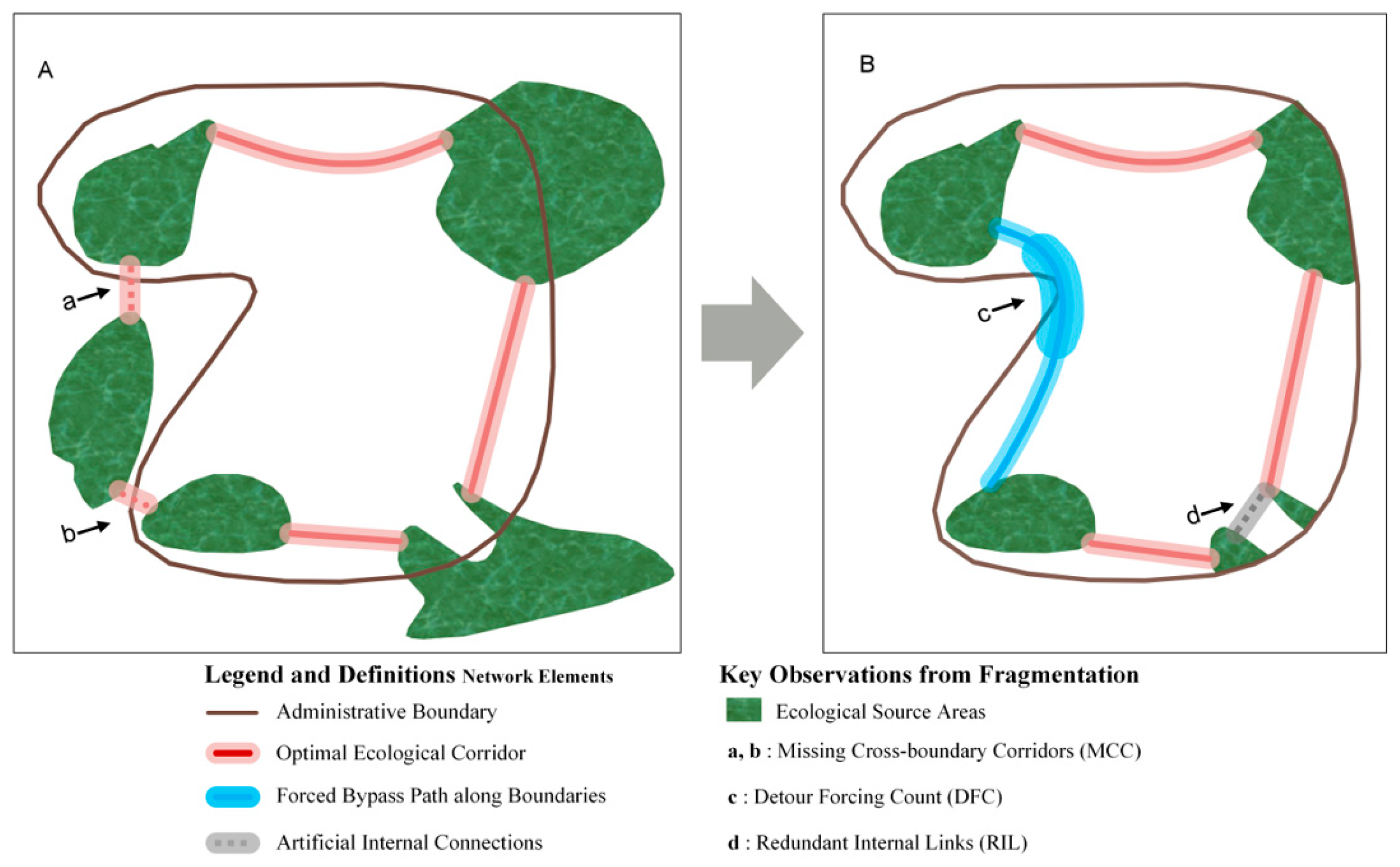
Figure 1. Conceptual illustration of administrative fragmentation effects on ecological networks. (A) Corridor connections between ecological source patches under unconstrained conditions; (B) corridor connections between ecological source patches when constrained by administrative-boundary fragmentation.
Forests 17 00611 g001
Figure 2. Spatial distribution and representativeness of the 30 selected counties in China. The main map shows county locations; the upper-right inset shows K-means clustering results; and the lower-right inset shows PCA ordination of all county-level units and selected counties. Red points indicate selected counties, and gray points indicate national county-level units (Section S1).
Forests 17 00611 g002
Figure 3. Methodological workflow. Rectangles: main steps; dashed boxes: sub-processes. Includes ecological network construction, metric calculation, and statistical analyses.
Forests 17 00611 g003
Figure 4. Frequency distributions of county-specific slope coefficients for six ecological network indicators across 30 counties. Slopes were estimated by regressing each indicator against log-transformed buffer distance. Negative values indicate decreases with buffer expansion, reflecting mitigation of administrative-fragmentation effects. Red dashed lines indicate mean slopes. (a) Frequency distribution of MCCslope; (b) Frequency distribution of DFCslope; (c) Frequency distribution of RILslope; (d) Frequency distribution of TCLslope; (e) Frequency distribution of MCRslope; (f) Frequency distribution of TEFCslope.
Forests 17 00611 g004
Figure 5. Structural equation model illustrating pathways from administrative fragmentation to total ecological flow cost. Solid arrows: significant; dashed arrows: non-significant.
Forests 17 00611 g005
Table 1. Standardized regression coefficients (β) of the best-fitting multiple linear regression models for the slope parameters of six ecological network indicators.
PredictorsMCCslopeDFCslopeRILslopeTCLslopeMCRslopeTEFCslope
SHID0.148 ***0.084−0.051−0.002
ELED0.099−0.257 *−0.022 *0.005
HMFT0.0420.321 **0
APRE−0.177 **−0.05−0.0160.003
TEMP0.224 ***0.060.00800.015
CLPR−0.199
FLPR−0.0470.029−0.340 ***−0.007−0.008−0.006
SLPR0.0160.119
GLPR0.017
ISP−0.0420.034−0.471 **
SHID × GLPR−0.041 **
TEMP × GLPR−0.002
TEMP × SLPR−0.024
HMFT × ISP−0.038
Adjusted R20.6430.2730.4770.3100.0880.480
Notes: Dependent variables are the slope values (rate of change with log-transformed buffer distance) of six indicators: MCC (Missing Cross-boundary Corridor), DFC (Detour Forcing Count), RIL (Redundant Internal Link), TCL (Total Corridor Length), MCR (Mean Corridor Resistance), and TEFC (Total Ecological Flow Cost). Independent variables include: SHID (Shape Index), ELED (Elevation Difference), HMFT (Human Footprint), APRE (Annual Precipitation), TEMP (Annual Mean Temperature), CLPR (Cropland Proportion), FLPR (Forest Land Proportion), SLPR (Shrub-land Proportion), GLPR (Grassland Proportion), ISP (Impervious Surface Proportion), and selected two-way interaction terms. Cells marked with “—” indicate the variable was not selected in the final model for that indicator (p ≥ 0.1). Significance levels: *** p < 0.001, ** p < 0.01, * p < 0.05. Adjusted R2 values are reported for each model.
Table 2. Standardized coefficients (β) from linear mixed-effects models assessing the effects of landscape, climate, and buffer distance on raw ecological network metrics.
PredictorsMCCDFCRILTCLMCRTEFC
BUFFER−0.412 ***−0.441 ***−0.613 ***−0.044 ***−0.021 ***−0.066 ***
SHID−0.554 ***−0.475 ***0.284 **−0.241 *
ELEM−0.453 *0.947 **−0.916 ***0.260 ***
TEMP−0.276 *−0.578 *0.172 **−0.755 ***
APRE0.268 *−0.103 *
CLPR1.459 *
FLPR1.056 ***
SLPR0.747 ***
HMFT−0.749 ***
GLPR−1.782 ***
ISP−1.050 *1.320 ***
BUFFER × SHID0.163 ***0.110 *
BUFFER × ELEM−0.019 ***
BUFFER × FLPR−0.264 ***
BUFFER × TEMP0.225 ***
TEMP × HMFT−0.070 *
TEMP × SLPR−1.650 ***
TEMP × GLPR−0.895 ***
SHID × GLPR−0.752 ***
HMFT × ISP0.662 *
Marginal R20.650.380.510.730.630.72
Notes: Dependent variables are the raw values (not slopes) of six ecological network metrics: MCC (Missing Cross-boundary Corridor), DFC (Detour Forcing Count), RIL (Redundant Internal Link), TCL (Total Corridor Length), MCR (Mean Corridor Resistance), and TEFC (Total Ecological Flow Cost). BUFFER is log-transformed buffer distance. SHID: Shape Index; ELEM: Mean Elevation; TEMP: Annual Mean Temperature; APRE: Annual Precipitation; CLPR: Cropland Proportion; FLPR: Forest Land Proportion; SLPR: Shrubland Proportion; HMFT: Human Footprint Index; GLPR: Grassland Proportion; ISP: Impervious Surface Proportion. Cells marked with “—” indicate the variable was not included in the final model for that metric or its effect was non-significant (p ≥ 0.05). Significance levels: *** p < 0.001, ** p < 0.01, * p < 0.05. Coefficients are shown to three decimal places. Marginal R2 values represent the proportion of variance explained by fixed effects. All models controlled for spatial autocorrelation and potential confounding variables, with “County” included as a random intercept.
Disclaimer/Publisher’s Note: The statements, opinions and data contained in all publications are solely those of the individual author(s) and contributor(s) and not of MDPI and/or the editor(s). MDPI and/or the editor(s) disclaim responsibility for any injury to people or property resulting from any ideas, methods, instructions or products referred to in the content.