Article

Functional Trade-Offs in Productive and Structurally Heterogeneous Forests: Insights from the Italian Alps

by
Federico Romanato
,
Silvio Daniele Oggioni
,
Matteo Vizzarri
* and
Giorgio Vacchiano
Dipartimento di Scienze Agrarie e Ambientali—Produzione, Territorio, Agroenergia, Università degli Studi di Milano, Via Celoria 2, 20133 Milan, Italy
*
Author to whom correspondence should be addressed.
Forests 2026, 17(4), 436; https://doi.org/10.3390/f17040436
Submission received: 27 February 2026 / Revised: 23 March 2026 / Accepted: 26 March 2026 / Published: 31 March 2026
(This article belongs to the Section Forest Ecology and Management)

Abstract

Forest structure is fundamental for linking ecological processes with management outcomes, and it influences key ecosystem services. However, the high cost and complexity of field data collection often limit the application of structural indices to small-scale studies, constraining operational assessments of forest multifunctionality. This study develops and tests an operational indicator of forest multifunctionality based on the structural heterogeneity index derived from forest management plans (FMPs). We analyzed the dendrometric data from 134 management units across 15 FMPs in the Lombardy region (Italy). Horizontal diversity was quantified using a Gini-based index, calculated from tree diameter-class distributions and combined with stand age, timber stock, and tree density using principal component analysis. Two orthogonal gradients emerged: a productivity gradient and a maturity–structural heterogeneity gradient. Generalized linear mixed models were used to assess their effects on carbon sequestration, timber yield, and touristic–recreational value. Structural heterogeneity was positively associated with all three functions, while productivity showed contrasting effects, particularly a negative relationship with recreational value. These results demonstrate that structural complexity and productivity are not necessarily in conflict and highlight the potential of FMPs as cost-effective data sources for operational, landscape-scale assessments of forest multifunctionality.

1. Introduction

Forest structure is fundamental for linking ecological processes with management outcomes, and it is recognized as a key component of sustainable forestry. Forest structure is one of the main attributes that affect ecosystem properties, including the provision of ecosystem services [1]. In fact, forest structure influences key ecological processes such as nutrient cycling, carbon sequestration, biodiversity conservation, and resilience to disturbances [2,3]. In general, forest structure refers to the configuration and distribution of different plant species and sizes within a stand [4]. However, the definition of forest structure is not unique and sometimes it appears ambiguous, as it can address different stand features (e.g., vertical layering, horizontal heterogeneity, or species composition). The spectrum of forest structures found worldwide is remarkably broad, ranging from oversimplified systems, such as even-aged plantations or intensively managed forests, to very complex systems, such as uneven-aged tropical rainforests. This variability reflects not only natural dynamics but also human intervention, making forest structure a fundamental concept for both ecological research and forest management [5]. Indeed, forest management is a key indicator of forest structure. By modifying structure and competition processes, forest management can impact a wide range of ecological processes, enhancing specific functions at the expense of others [6]. Different structural parameters are associated with different functions [7]. Although analyzing and classifying forest structures can help identify the best possible function for a stand, applications are often site-specific and difficult to upscale [8,9].
This variability also manifests at much smaller spatial scales: for example, in Lombardy (Northern Italy), forest structure varies substantially depending on geomorphology, forest type, elevation, and management regime. The Italian National Forest Inventory [10] documents marked spatial variability in forest quality, composition, and forest types, while at the same time indicating a broadly balanced distribution of forest categories at both the regional scale and along the altitudinal gradient. Importantly, this balanced pattern also emerges for several key structural parameters such as growing stock volume, volume increment, canopy cover, tree density, and stand age, suggesting a high variability of forest structural complexity across the region.
Defining and measuring structural complexity and developing corresponding indices is not straightforward [9,11,12]. Stand structural complexity is essentially a measure of the variety of structural attributes (e.g., abundance, relative abundance, richness, size variation, and spatial variation in different forest variables) and the relative abundance of each attribute [13]. This requires the collection of extensive forest data, preferably in the field, for higher precision. Due to the complexity and high costs of field data acquisition, it is sometimes necessary to build indices of structural complexity from other, less detailed data sources (e.g., forest management plans), but no standardized procedures currently exist for this purpose [14,15,16], resulting in considerable variability among studies and regions in both what is measured and how it is assessed [17]. Additionally, differences in spatial scale, data availability, and institutional capacity hinder uptake. Filling this gap—through validation studies, stakeholder engagement, and development of standard operational frameworks—is key to ensure that structural complexity metrics inform real management and policy decisions.
In this study, we propose a comprehensive index of structural heterogeneity (SHI) based on stand dendrometric parameters obtained from the forest management plans (FMPs) in different Italian alpine forests to provide a tool supporting operational management planning. The aim of this study is to test the SHI based on the data derived from FMPs and to identify the main variables that drive structural heterogeneity in forest ecosystems. The study also explores the relationship between the SHI and different forest functions, with the broader goal of evaluating its potential as a practical tool for supporting forest planning, management, and the assessment of ecosystem services.
We focused on Italian alpine forests since they represent a key component of the European forest landscape due to their ecological, economic, and social importance. Indeed, they provide a wide range of ecosystem services, including: timber provision, carbon sequestration, water regulation, mitigation of natural hazard, biodiversity conservation, and provision of non-timber product [18,19,20]. Historically, these forests have been managed under multifunctional principles, balancing productive, protective, and ecological objectives [21]. However, in recent decades, their structure and functionality have been increasingly threatened by the combined effects of climate change, land abandonment, and changing socio-economic conditions [19,22]. These dynamics make Alpine forests an ideal case study for investigating how forest structure can impact the provision of different ecosystem services.
To our knowledge, this is among the first attempts to systematically apply a structural heterogeneity derived from the management plan data in Alpine forests, aiming to bridge the gap between ecological theory and operational forestry.

2. Materials and Methods

2.1. Study Area

This study focuses on two Alpine valleys located in the Lombardy region (Northern Italy): Valle Camonica and Valchiavenna. These sites (Figure 1) were selected due to the high availability and completeness of forest management plan data, which was essential for the analysis.
Valle Camonica is one of the largest valleys in the Central Alps, extending approximately 100 km in length and covering a total area of 1365 km2. The elevation ranges from 250 m to 3539 m a.s.l., with the highest point at Mount Adamello. Forests cover 648 km2 of the valley, representing approximately 14% of the total forest area in Lombardy. The dominant forest types are composed of chestnut (Castanea sativa) and Norway spruce (Picea abies) [23,24]. Sweet chestnut forests predominantly occur at lower elevations, ranging from 300 to 1000 m above sea level (a.s.l.), more adapted to warmer conditions and fertile soils. As elevation increases, the forest composition shifts mainly toward Norway spruce, which is well-adapted to the cooler and more acidic soils found at higher elevations (1000–1800 m a.s.l.). Above 1800 m, forests are primarily characterized by a mix of alpine species such as larch (Larix decidua) and Swiss pine (Pinus cembra), often interspersed with subalpine meadows and shrubland [24]. The climate is classified as sub-oceanic, and the valley is mainly characterized by morainic soils. Approximately 25% of the valley’s surface is used for agriculture, with predominant cereal and forage crops. Valle Camonica also includes several Natura 2000 sites, providing protected habitats for local biodiversity.
Valchiavenna is a transboundary Alpine valley covering 574 km2, bordering both the Lombardy region and the Swiss Canton of Grisons. It includes two sub-valleys: Val Bregaglia, where the Mera River originates, and Valle Spluga, drained by the Liro stream. Forests occupy about 209 km2, accounting for 36% of the valley’s total surface [23]. These forests are composed of 55.9% high forests and 44.1% coppice stands. The dominant species include chestnut, Norway spruce, and European larch. Like in Valle Camonica, the distribution of tree species in Valchiavenna is strongly influenced by an altitudinal gradient. At lower elevations (300–1000 m above sea level), chestnut and oak (Quercus spp.) dominate, while, as elevation increases, the forest composition shifts towards montane ecosystems, where Norway spruce and larch become more prevalent. Above 1500 m, Swiss pine and larch are the main species. At higher elevations, forest cover gradually gives way to pasturelands and, ultimately, to bare rocky landscapes [25]. The valley has an Alpine climate, characterized by a wide altitudinal gradient.

2.2. The Data from Forest Management Plans

In order to investigate the relationship between structural forest heterogeneity and ecosystem services, we first digitized forest management plans. The data used for the analysis in this study were collected from the forest management plans (FMPs) in the study area (Valle Camonica and Valchiavenna). The available FMPs can be accessed freely on Lombardy’s digital library of forest management plans [26]. Between all the available FMPs, we selected only those located in the study area (Table A1), currently in force or due to expire, with clearly reported forest data according to ‘management unit’ division, and which did not contain drafting errors, such as typing errors, incorrect numbers, or missing tables. The choice of management plans useful for data collection led to the selection of 15 FMPs, of which 13 are located in the province of Brescia (BS), relating to Valle Camonica, and two are located in the province of Sondrio (SO), relating to Valchiavenna. Of the 15 plans taken into consideration, seven will expire after 2030, six between 2025 and 2030, and two expired in 2024 and have not yet been renewed (Table 1).
Each forest plan covers multiple management units (Table 1), which were considered as study units for this work. A total of 134 management units have been found between the selected FMPs. For each management unit, we extracted average diameter at breast height (DBH), tree density (n stems/ha), forest species, mean stand age, total timber stock (m3/ha), and the distribution of trees into three diameter classes (17.5 cm ≤ DBH < 32.5 cm: small plants, 32.5 cm ≤ DBH < 52.5 cm: medium plants, and DBH ≥ 52.5 cm: large plants). Thus, while this simplification may introduce some bias and limit the representation of fine-scale structural variability, it reflects the structure of the data available in forest management plans. This allows for consistent application of the method across all management units although at the expense of detailed structural resolution.

2.3. Building the Structural Heterogeneity Index

To evaluate structural forest heterogeneity, we calculated the horizontal diversity index (HDI) for each management unit based on the Gini index, calculated on the frequency distribution of trees across the three diameter classes. The Gini index, initially developed in economics, is a statistical measure of distribution inequality [27], and it is particularly useful for analyzing classical forest inventory data, such as height or DBH, divided into classes [17,28]. The Gini coefficient (G) was calculated using the standard formulation based on pairwise differences among class values:
G   =   [ sum   over   i   sum   over   j   of   | x i   −   x j | ] / ( 2   n 2   x ¯ )
where xi and xj represent the number of trees per hectare in the i-th and j-th diameter classes, n is the number of classes (n = 3), and x ¯ is the mean number of trees across classes.
To enhance interpretability, Gini values were reversed (1 − Gini), so that higher HDI values reflect greater structural complexity.
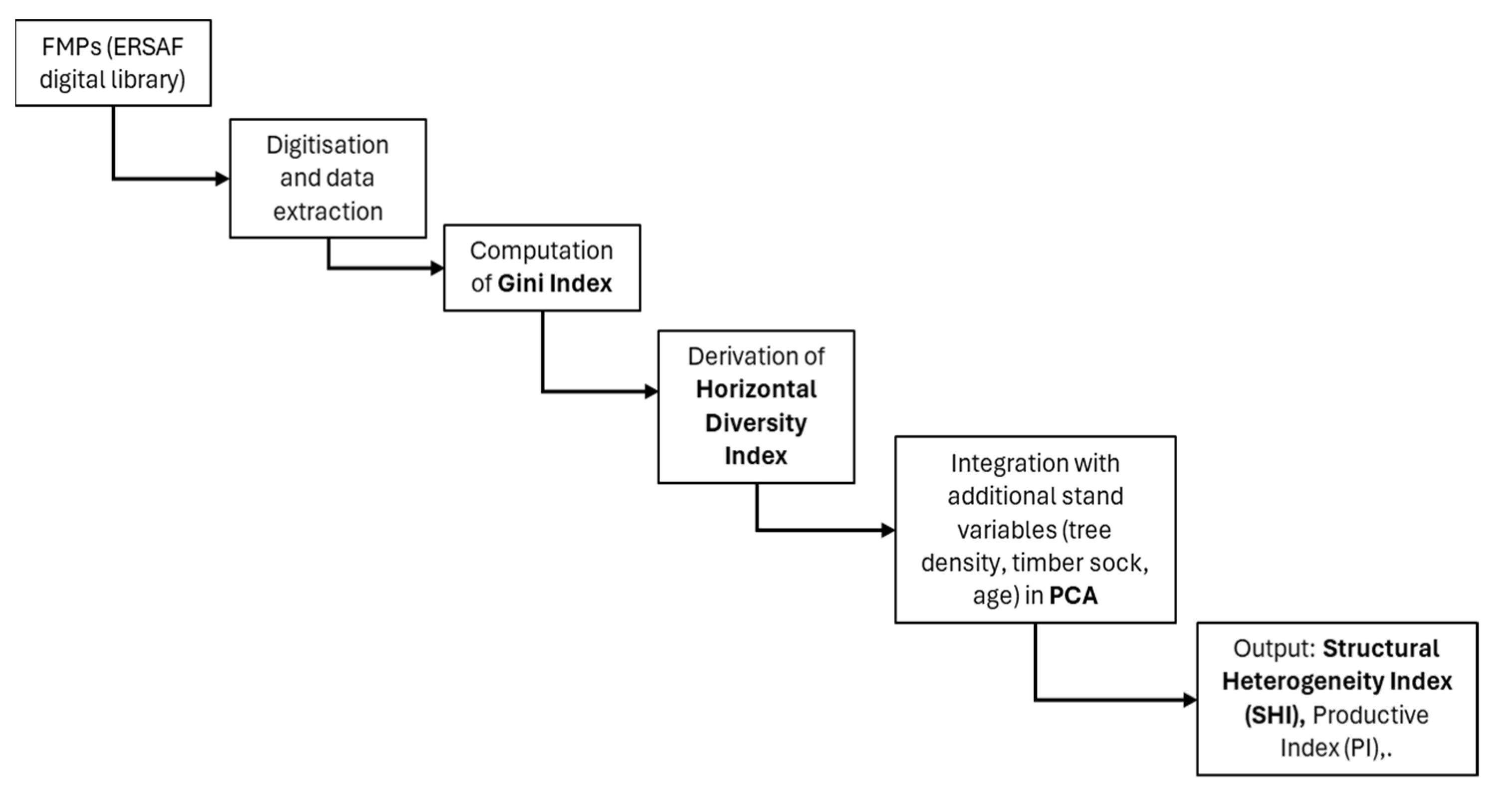
However, it is generally agreed that the Gini coefficient alone is insufficient to analyze complex forest structures, as it fails to capture the full range of structural heterogeneity in these ecosystems [15,17]. To incorporate greater environmental variability into the analysis, we performed a principal component analysis (PCA) that included four variables describing different structural aspects of forest ecosystems: HDI, mean stand age, total timber stock per hectare, and tree density per hectare. Although these variables represent partially different ecological dimensions (e.g., structural heterogeneity, stand development, and productivity), they are interconnected within forest stand dynamics. In managed forests, these variables are typically shaped by the development stage and silvicultural history and can therefore be interpreted as indirect proxies of structural conditions. Their joint use thus complements the Gini-based HDI, allowing a more comprehensive representation of forest structure. The resulting axes from the PCA, which explain the latent gradients of ecological dynamics, will be used as explanatory variables in the analysis of the productive and tourist/recreational functions of the forests of Valcamonica and Valchiavenna. The use of PCA does not imply a strict separation among these dimensions but rather identifies dominant gradients of variation in which different attributes contribute with varying weights. The workflow of the procedure is summarized in Figure 2.

2.4. Assessing the Effects of Structural Heterogeneity on Forest Functions

With FMP as the data source, collecting precise indicators of ecosystem services (ES) is challenging. However, a literature review allowed us to identify and adopt three variables as proxies, each representative of a given forest function: CO2 sink (tCO2 −1 ha−1 year−1), timber yield (m3 ha−1), and tourism–recreation value. As the direct measurement of TR value was not available, we adopted an expert-based scoring approach derived from the literature [29]. Although this may introduce some degree of subjectivity, the scores are based on a structured expert framework and are consistent with established evidence on the influence of forest management and species composition on recreational value.
We refer to these proxies as forest functional traits (FFT) (Table 1).
Table 1. Forest functional trait (FFT) explanation.
FFTUnitsData Origin and ExplanationES ClassSupporting Literature
CO2 sinktCO2 ha−1 year−1CO2 sink was estimated from annual volume increment per hectare using the following equation:
CO2 sink = INCR_HA × WD × BEF × CF × 3.67,
where INCR_HA is the annual increment in stem volume (m3 ha−1 year−1), WD is wood density (t m−3) of the dominant tree species, BEF is the biomass expansion factor, CF is the carbon fraction of dry biomass (assumed equal to 0.5), and 3.67 is the molecular weight ratio used to convert carbon into CO2.
Species-specific values of wood density and BEF were assigned according to the dominant species recorded for each management unit [30].
Regulation[31]
Timber yield/provisionm3 ha−1It represents the harvestable provision defined directly by forest managers (considering fertility, increment, age, etc.)Provisioning[32]
Touristic–recreational value (TR)Score (0–10)It is derived from a literature-based matrix, where recreational scores are assigned to forest stand types based on species, development stage, and management regime. The scores were obtained through a structured Delphi survey of European experts and represent a standardized proxy for cultural ecosystem services.Cultural[29]
To analyze the effect of structural heterogeneity on prevailing forest functions, we fitted generalized linear mixed models (GLMMs) to the three FFTs. We used the first two axes resulting from the PCA and four environmental covariates (slope, elevation, aspect, mean annual temperature, and cumulative growing-season precipitation) as predictors. Aspect was included as the cosine of the aspect angle, yielding a continuous variable from −1 (south-facing) to 1 (north-facing). Collinearity among predictors was evaluated through the variance inflation factor (VIF); variables with VIF > 10 were excluded. Mean temperature was removed from the predictors because of high collinearity with elevation (VIF = 17.2–18.7).
Because each FFT represents a distinct ecological process, we adopted a model formulation with trait-specific parameters. For each trait, k (CO2 sink, timber yield, and tourism–recreation), and each management unit, i, the linear predictor is defined as:
ηk,i = αk + βk1 PCA1i + βk2 PCA2i + βk3 Slopei + βk4 Elevationi + βk5 Aspecti + βk6 Precipitationi + uk,p(i)
where uk,p(i) is a random intercept associated with the forest management plan (FMP), p, accounting for the nested data structure. PC1 and PC2 are the two axes resulting from PCA, which express specific gradients.
uk,p ∼ N(0,σ2 u,k)
The expected value of each FFT depends on the distributional family:
Gaussian model (link = identity) for recreational value.
Gamma model (link = log) for CO2 sink and timber production.
All statistical analyses were performed using the R software (version 4.4.3) (R Core Team, Vienna, Austria). The Gini coefficient was calculated using the ineq package [33]; the principal component analysis (PCA) was performed with the base R function, prcomp; generalized linear mixed models were fitted using the glmmTMB package [34], collinearity was assessed with the car package [35]; model explanatory power was evaluated using the performance package [36]; and partial regression plots were produced with visreg [37].

3. Results

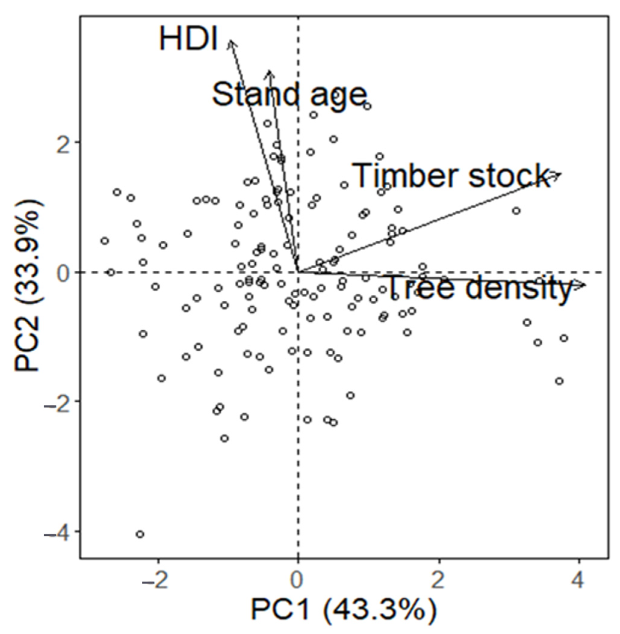
The PCA identified two dominant axes of variation (Figure 3). The first principal component (PC1) explained 43.3% of the total variance, while the second component explained (PC2) 33.9%
PC1, hereafter referred to as the productive index (PI), was strongly positively associated with a productivity gradient, showing high loadings for timber stock and tree density. In contrast, PC2, hereafter termed the structural heterogeneity Index (SHI), reflected a gradient of increasing stand maturity and structural complexity (Table 2). Given their clear ecological interpretation and high explanatory power, the PI and SHI were directly included as predictors in subsequent modeling.
It is important to note that, although the PC1 and PC2 can be interpreted respectively as productivity and structural heterogeneity gradients, the contribution of individual variables is not exclusive. Most variables show loadings that contribute to both axes. In fact, timber stock, mainly associated with the PC1, also slightly contributes to the PC2, whereas the HDI, followed by stand age, which primarily drive the PC2, show minor contributions to the PC1 (Table 2). This indicates that both components integrate information from all variables, although with different relative weights.
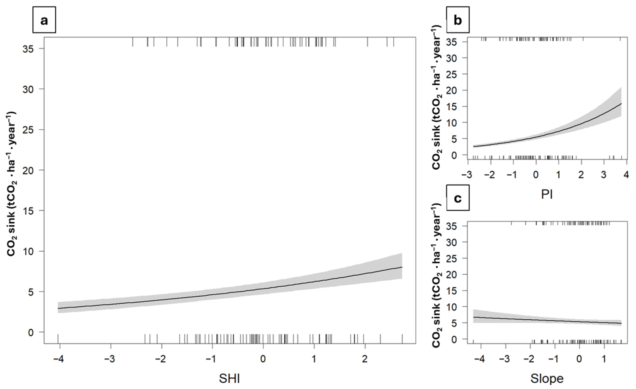
The GLMMs with Gamma distribution revealed that CO2 sink was significantly and positively associated with both principal component axes (Figure 4). The PC2 (structural heterogeneity index) was positively associated with CO2 sequestration (estimate = 0.15 ± 0.02 SE, z = 5.98, p < 0.001) (Figure 4a). The PC1 (productive index) showed the strongest effect (estimate = 0.28 ± 0.03 SE, z = 9.64, p < 0.001) (Figure 4b). Slope showed a weak negative effect (estimate = −0.05 ± 0.03 SE, z = −1.57, p = 0.116), while elevation, aspect, and precipitation had no detectable influence (Figure 4c) (Table A2). The model explained a substantial proportion of variability, with a conditional R2 of 0.778 and a marginal R2 of 0.473.
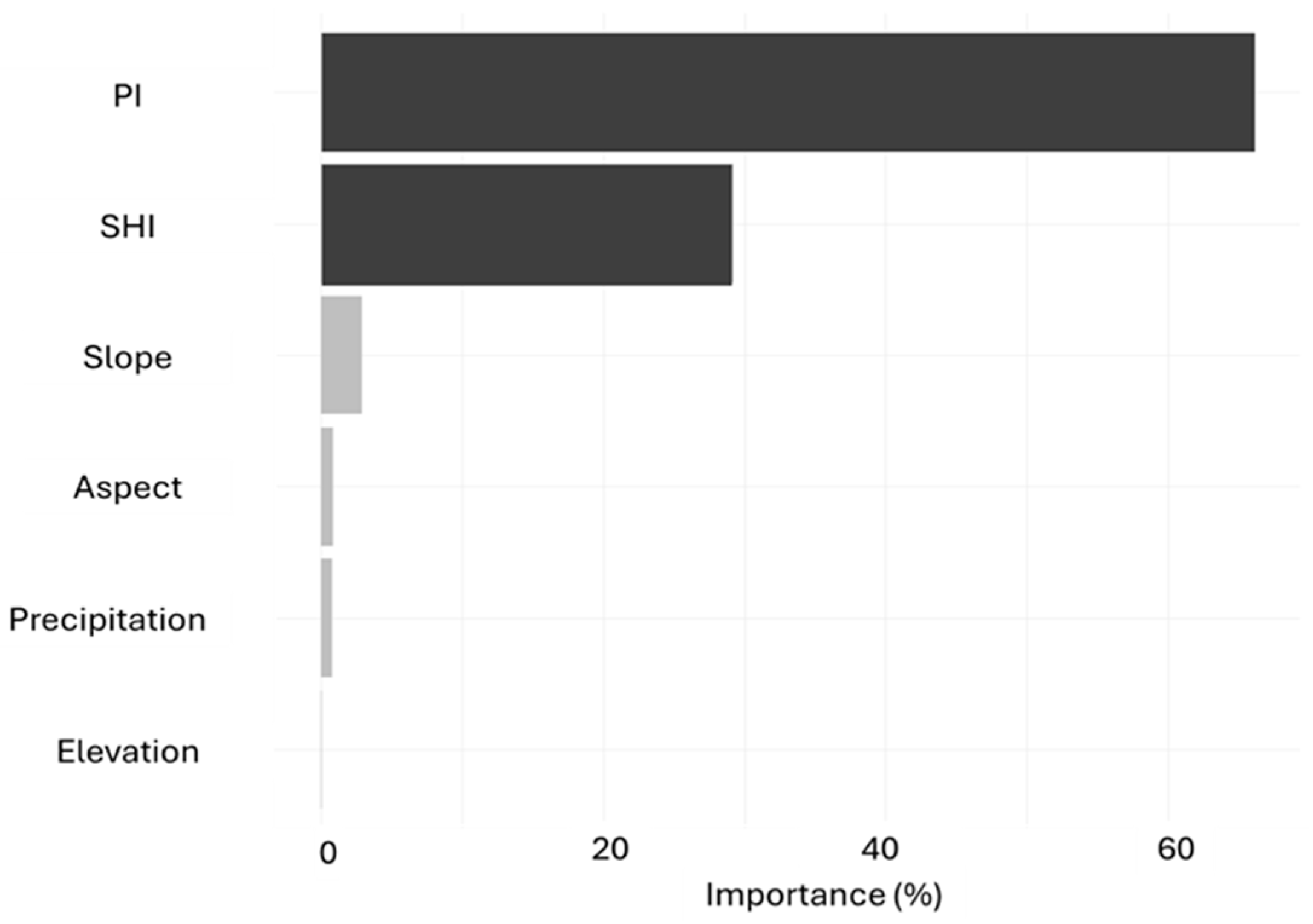
Variable importance analysis for the Gamma GLMM indicated that CO2 sink capacity was driven by the PI, which accounted for approximately 66% of total model importance (Figure 5). The SHI contributed 29%, suggesting that more structurally developed stands also enhanced carbon sequestration potential. In contrast, slope, aspect, precipitation, and elevation each explained less than 5% of the variation, indicating negligible effects on CO2 sink strength.
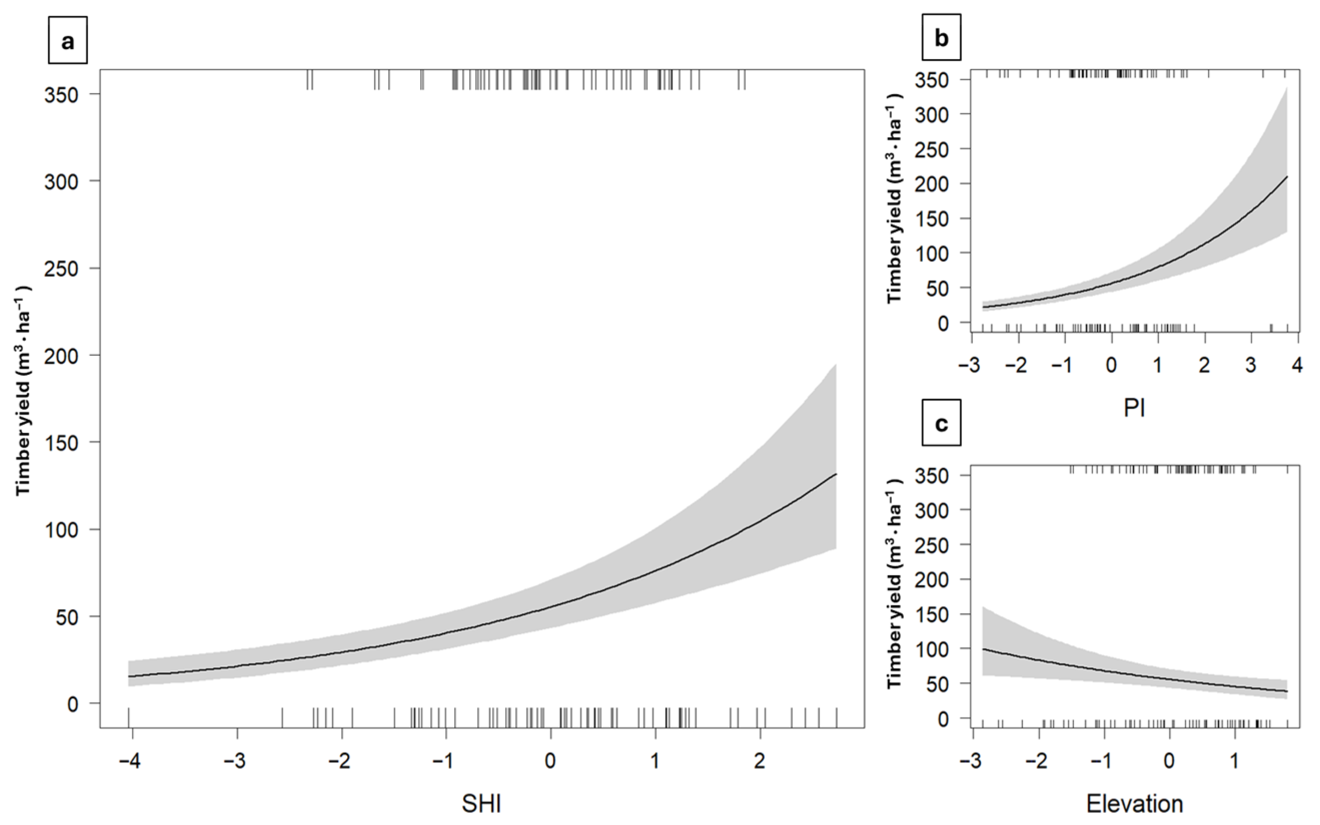
The Gamma GLMM with a log-link revealed that timber yield was strongly and positively associated with both principal components-derived indices (Figure 6). The structural heterogeneity index showed a significant positive association (estimate = 0.32 ± 0.05 SE, z = 6.12, p < 0.001) (Figure 6a). The productive index had the strongest effect (estimate = 0.35 ± 0.05 SE, z = 7.15, p < 0.001) (Figure 6b).
Among the environmental covariates, elevation exerted a significant negative effect (estimate = −0.20 ± 0.07 SE, z = −2.79, p = 0.005) (Figure 6c). In contrast, slope, aspect, and precipitation showed no detectable influence on stand recovery (all p > 0.2) (Table A2).
Model explanatory power was moderate to high, with a conditional R2 of 0.671 and a marginal R2 of 0.543.
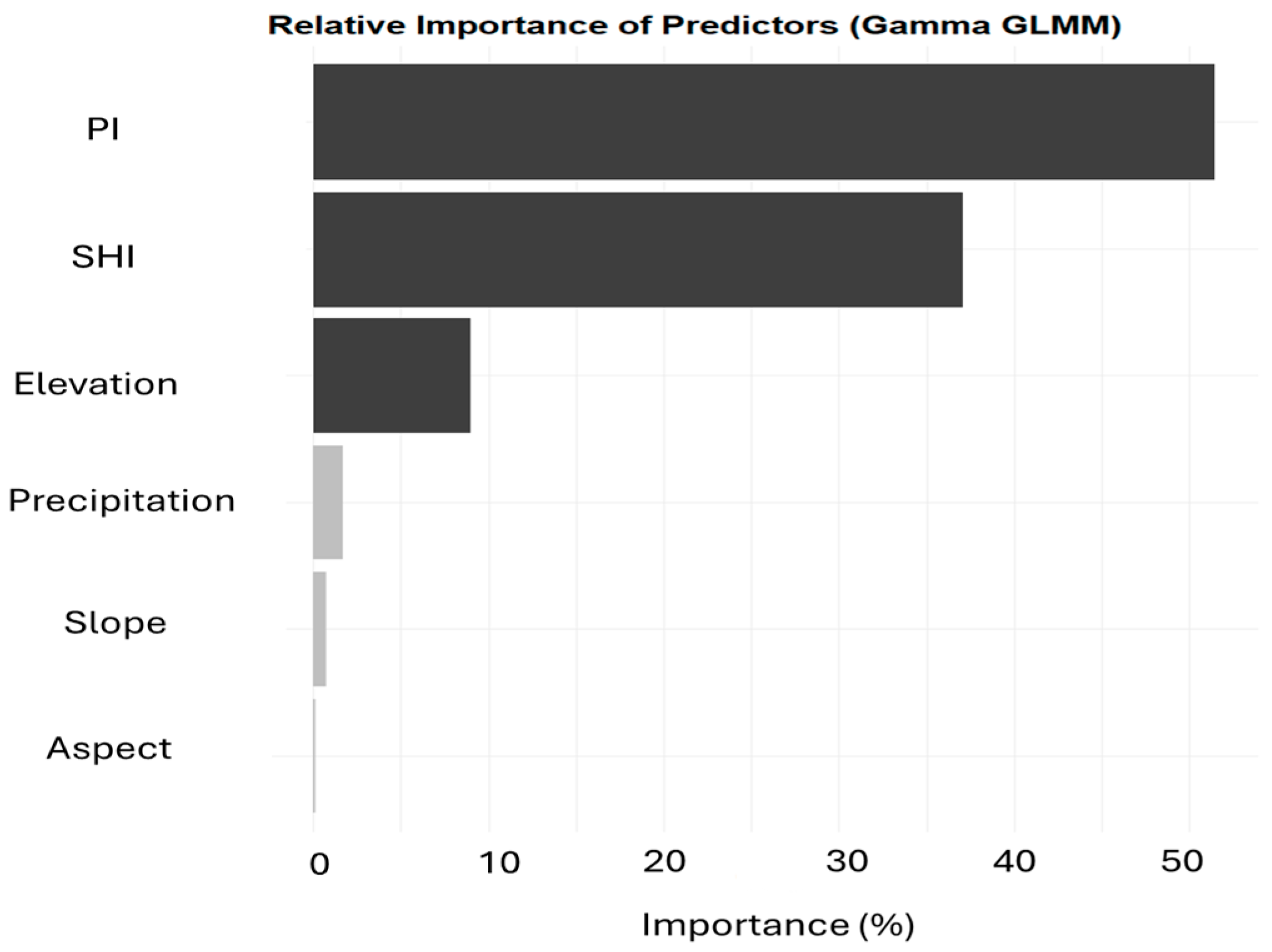
Variable importance analysis for the Gamma GLMM indicated that timber yield was primarily driven by the PI, which accounted for approximately 51% of the total explanatory power (Figure 7). The SHI followed with 36%, suggesting a strong but secondary influence. Elevation contributed moderately (≈9%), while precipitation, slope, and aspect each explained less than 2% of the variation, indicating minimal effects on timber yield.
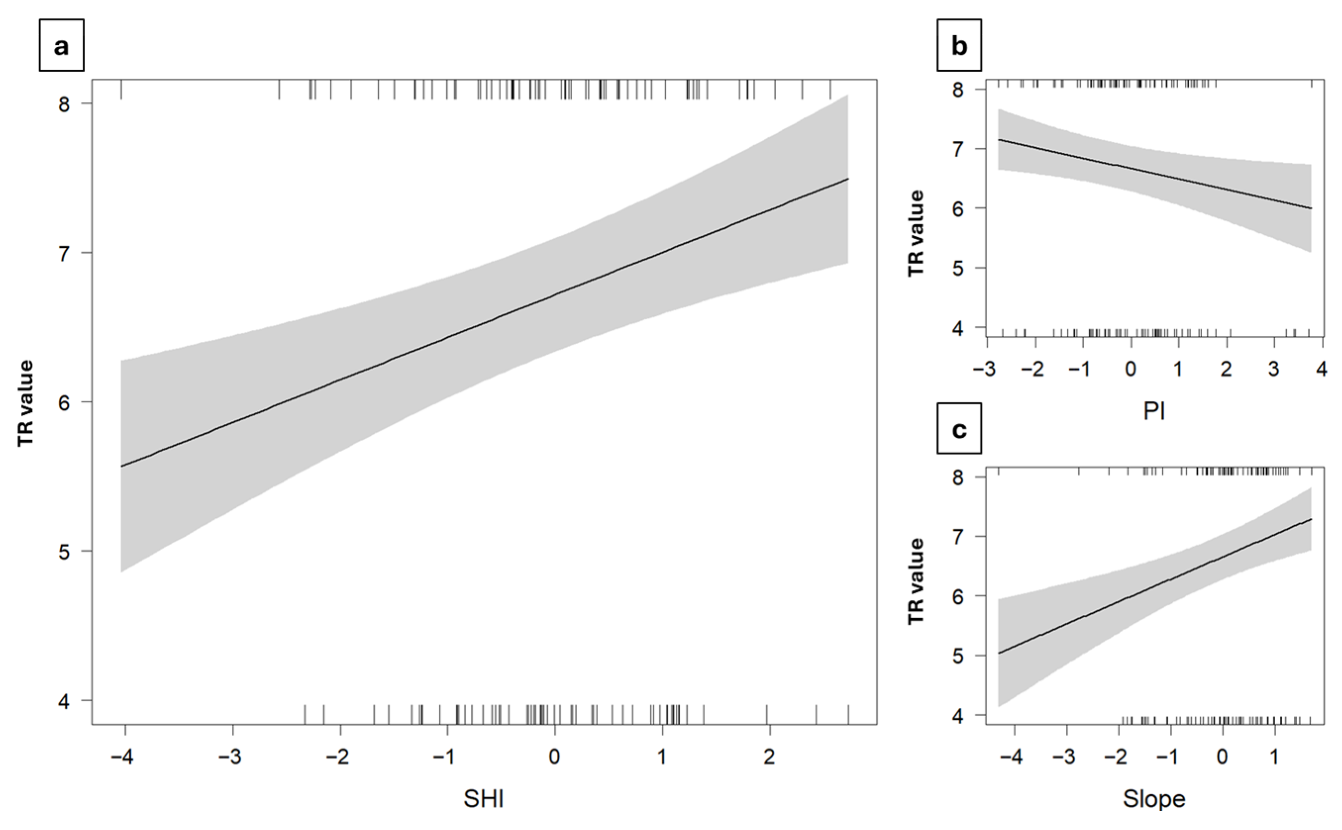
The Gaussian GLMM revealed that touristic–recreational value was significantly influenced by both stand productivity and structural heterogeneity (Figure 8). The structural heterogeneity index had a positive and significant effect (estimate = 0.28 ± 0.08 SE, z = 3.71, p < 0.001) (Figure 8a). Conversely, the productive index showed a negative effect (estimate = −0.18 ± 0.08 SE, z = −2.32, p = 0.020) (Figure 8b).
Among the environmental predictors, slope exerted a strong positive influence (estimate = 0.38 ± 0.10 SE, z = 3.68, p < 0.001) (Figure 8c). Elevation, aspect, and precipitation showed no detectable effects (all p > 0.3) (Table A2).
Model explanatory power was modest, with a conditional R2 of 0.378 and a marginal R2 of 0.287.
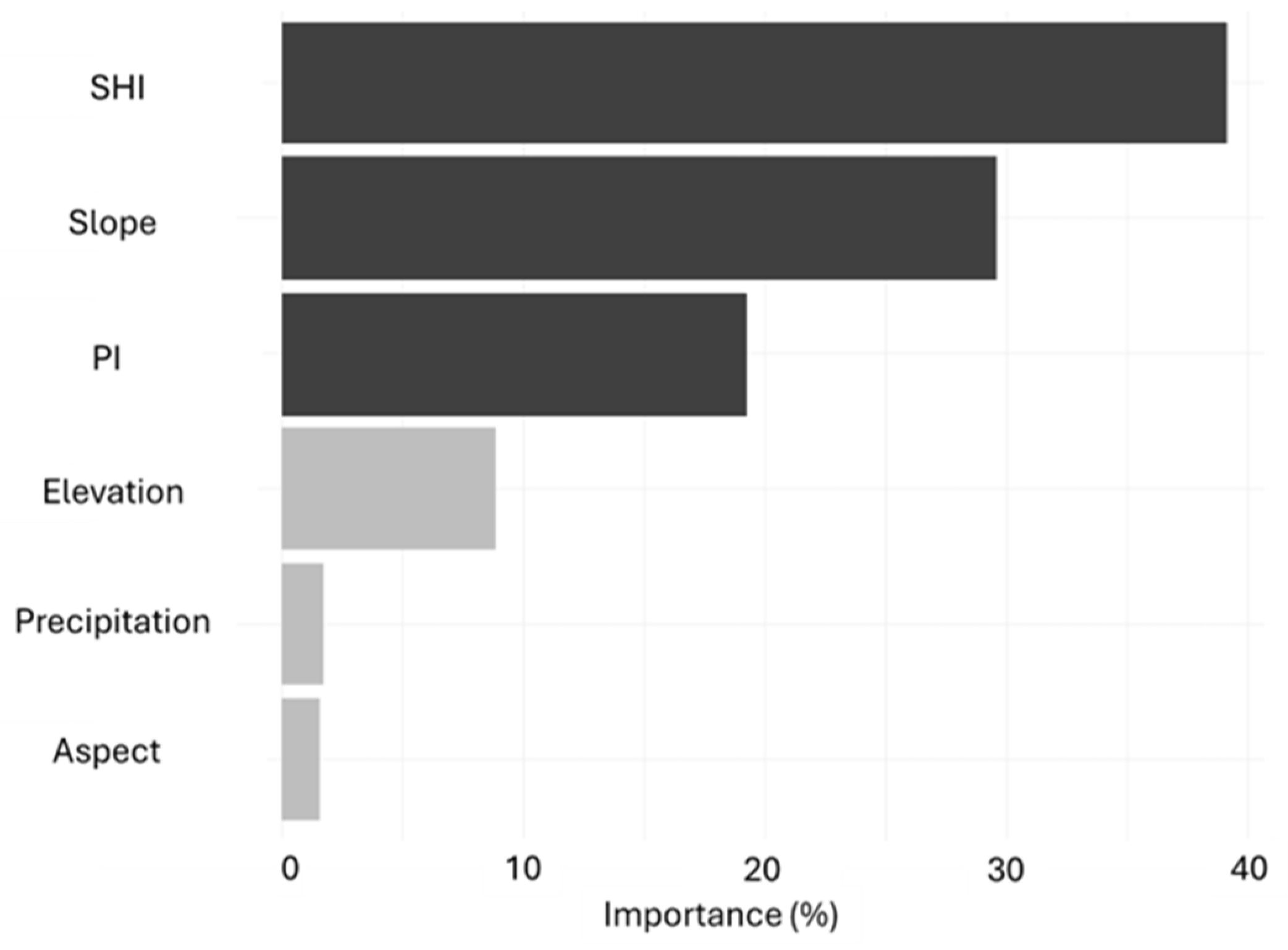
The analysis of variable importance (Figure 9) highlights the relative contribution of different predictors to the tourism–recreation GLMM. The SHI was the strongest predictor, accounting for approximately 39% of total model importance. The slope and PI followed, contributing 29% and 19%, respectively. Elevation showed a moderate influence (≈8%), while precipitation (≈2%) and aspect (≈1%) had only minor effects.

4. Discussion

4.1. Multivariate Structural Gradients

The PCA results show that the considered variables (stand variables) are organized along two principal gradients, one ecological/productive and one structural. The PC1 axis corresponds to the quantitative/productive variables (PI); it represents more than 40% of the variance, and it is related to the productivity of the stands since it mainly follows the timber stock and tree density variables. The observed association between timber stock and tree density (PC1) aligns with classical stand dynamics theory, where stand density regulates resource partitioning and biomass accumulation [38,39].
The second axis (PC2), which captures one-third of the variance, reflects instead a maturity and structural heterogeneity gradient. Indeed, the positive association between the SHI and stand age suggests that the SHI may effectively catch the dimensional differentiation process that develops with the aging of a stand cycle. This is particularly relevant, as it indicates that even a simple index obtained from forest management plans is able to provide crucial information about structural complexity, normally considered accessible only through more detailed field data [13].
The two main axes represent distinct ecological dimensions, with the productivity index (PC1) primarily capturing biomass-related variation and forest density, while the structural heterogeneity index (PC2) is largely driven by the HDI and stand maturity. Even though the PC2 retains a minor component of standing stock, the principal gradient of timber quantity remains orthogonal to structural variability. Forest structural heterogeneity has often been linked to stand productivity or biomass accumulation [1,13]. However, recent studies suggest that this assumption can lead to misleading results and may overlook some important ecological dynamics. Structural attributes such as size difference, spatial variability, or age diversity are strongly influenced by stand development dynamics, disturbance history, and management practices rather than by biomass alone [11,13,17]. Therefore, structure diversity and productivity can become decoupled: highly productive forests may show low structural complexity, whereas structurally diverse stands do not necessarily correspond to high-growing stock or density [2,40]. Our PCA results provide empirical support for this conceptual separation. This decoupling allows a more precise interpretation of forest complexity, confirming that structure and productivity can be analyzed, at least partially, as independent drivers of forest functioning.
The partial overlap among variables reflects that forest structure is the result from the interaction of stand development, competition processes, and management history [13]. In managed forests, attributes traditionally associated with productivity, such as growing stock and density, also reflect structural conditions and past silvicultural interventions. Therefore, their inclusion contributes to a more integrated representation of stand structure. From the ecological point of view, it is clear that structural heterogeneity is not a simple result of productivity, but it is linked with the life-cycle of the stands and its influence (disturbances, management, aging, etc.). From the management perspective, it highlights how the increase in structural complexity (using particular practices such as Closer to Nature Forest Management—CNFM) can require different approaches than those applied only to improve timber production. Eventually, from the scientific perspective, the non-collinearity between the SHI and PI represents promising results since they can be applied as complementary indicators for stand structure.

4.2. Structure as Ecosystem Service Predictor

The second form of decoupling, in addition to the divergence in productivity and structural diversity as a result of the PCA, emerges when considering the relationships between forest attributes and ecosystem functions. It is increasingly recognized that different functions respond to different components of forest structure: biomass-based functions such as timber yield or carbon sequestration tend to depend more strongly on quantitative attributes such as stand density, basal area, or growing stock, whereas functions related to biodiversity conservation, habitat provisioning, or resilience to disturbances are more closely associated with structural heterogeneity, spatial variability, and the presence of uneven-aged features [1,2,40]. Our results are consistent with this framework: while both gradients (SHI and PI) influence the three analyzed functions, their effects are distinct and sometimes contrasting, underscoring that ecosystem services are not uniformly governed by the same structural attributes. Recognizing this decoupling is essential for interpreting multifunctionality in managed landscapes, suggesting that higher structural complexity may support both ecological and cultural functions without necessarily mirroring the dynamics of biomass accumulation or productivity.
In detail, the first results from the GLMM (Figure 4) showed a positive and significant correlation between the C sink and both maturity and productivity gradients. The results related to the PI were predictable since a higher timber stock is more prone to sequester C from the atmosphere [41]. However, a correlation with the SHI may suggests that not only younger and denser forests have high absorptive capacity for carbon but also older and structured ones. This is in line with the evidence that more structured forests (e.g., old-growth forest—OGF) are not carbon-neutral, but they work as carbon sinks [42]. Although more structurally heterogeneous forests in our study do not qualify as old-growth forests, our analysis of the maturity and structural gradient suggests that structural heterogeneity may play a role in carbon sequestration. Furthermore, the overall results suggest that in our stands, the management adopted is already moving toward closer-to-nature management, and the results suggest that increasing structural complexity does not necessarily reduce carbon sequestration [43].
Model results (Figure 5) also underscore a positive correlation between timber yield and the two gradients resulting from the PCA but also a negative correlation with elevation. These outcomes are striking since the timber yield is calculated in the forest management plan, taking into account the current timber increment and also the economic necessities. The strong effect of PI was expected, as higher stocking and tree density are directly linked to greater volumes available for harvest, in line with classical yield theory and the central role of stand density in determining allowable cut [16]. The positive effect of SHI is particularly noteworthy, since it shows that structurally heterogeneous and mature forests are not only sustaining carbon sink but also timber yield and, thus, harvestable production. This result suggests that management approaches aligned with CFNM may not necessarily conflict with timber provision, and it and may contribute to stabilizing production [1]. The negative correlation with elevation supports the well-known confirmed theory according to which the elevation influences the timber yield of forests. This is probably due to several factors that are linked with elevation (soil and water availability, temperature, irradiation, etc.), but this result underlines the importance of accounting for site-specific constraints when interpreting yield models and designing forest management strategies.
Finally, the third model (Figure 6) revealed a contrasting pattern for the touristic–recreation value compared to carbon sink and timber yield. The SHI reveals a positive correlation with the TR values, showing that more complex and mature forests are perceived as more attractive, in line with studies showing that heterogeneous, multi-layered canopies and the presence of large trees enhance recreational quality and landscape appreciation [44]. However, the negative correlation with the PI underlines the mismatch between production and esthetic value. This is probably due to the rising awareness in public opinion about the real aspects of the naturalness and wildness of forests. Many studies confirmed how the perception of beauty in forest stands is driven by several factors, including the dendrometric ones [45,46], and they confirmed that more structured and older forests are normally considered more esthetic. Thus, our results suggest that recreational value may be approximated using data derived from management plans. Furthermore, it is important to evidence that the TR value is positively correlated with slope, which may reflect the difficulty of managing forests in steep mountainsides.

4.3. Forest Management Plans as Ecological Data Source

Our findings indicate that alpine forests show that structural diversity and heterogeneous stand conditions are indeed crucial for sustaining and enhancing multiple ecosystem services. Forest management plans can serve as readily available sources of forest data, requiring no additional field sampling efforts—apart from the time needed for the digitalization. A similar approach has been previously applied to the data collected following the Forest National Inventory protocol [9], but the complexity of data collection and analysis does not allow it to work on wider areas.
The use of data provided by forest management plans represents an innovative opportunity to obtain forest information without the need for specific field sampling campaigns, thereby reducing both costs and time requirements. This approach has several strengths: the availability of forest data for many areas across the country, collected by expert technicians, and referring to a fine spatial scale (single municipalities or small groups of municipalities). In addition, management plans are periodically updated (typically every 15 years), which also enables the study of historical forest dynamics. However, it is important to underline that the data from FMPs may not always capture the full structural variability of stands, particularly where diameter distributions are only partially reported or simplified. This gap is especially relevant in forests that are predominantly young or recently managed, where the absence of larger diameter classes may lead to an underestimation of structural complexity. Moreover, some drawbacks exist, such as the application of different data collection methods (e.g., relascope surveys vs. complete dendrometric surveys), the emphasis on productive stands where data collection is more detailed, and the heterogeneity in the structure of management plan documents. The latter often requires manual digitalization, as they are not standardized in digital formats, particularly if multiple plans are to be processed together. Furthermore, the use of these plans is limited to the areas where they are legally in force, and they generally do not cover private properties.
Moreover, several limitations occur when adopting FMP data, mainly because they are written by forest technicians and designed for administrative and silvicultural purposes. The accuracy and consistency of these data are not comparable with more scientific purpose data sources. For instance, in FMPs, crucial attributes related to structural complexity, such as deadwood amount, understory complexity, and microhabitat, are not taken into account. Moreover, the FMPs are periodically revised, and if on one hand, this ensures a regular update of the data, on the other hand, it limits the ability to capture short-term dynamics. Taken together, these limitations do not reduce the value of FMPs, but they highlight the need to interpret structural metrics with caution. In fact, the heterogeneity captured by data derived from FMPs is often biased toward younger, regularly managed forests and may therefore underestimate the structural complexity typical of mature, conservation-oriented, or old-growth stands. Finally, differences in standards and formats across regions may hinder large-scale comparability.
Furthermore, a methodological consideration involves using three diameter classes to calculate the Gini index and, consequently, the HDI. The Gini coefficient is a widely accepted measure of tree size inequality in forest structural analysis [47,48]; however, its use with aggregated diameter classes rather than individual tree measurements may not capture detailed structural variability. This choice is intentional: our study uses the FMP data to assess structural heterogeneity at the landscape scale, consistent with a well-established tradition of deriving ecological indicators from standardized inventory and planning data [49,50]. This method ensures spatial coverage, temporal consistency, and direct applicability to operational forest management, which would be difficult with plot-level dendrometric surveys alone. Future research could compare FMP-derived and tree-level structural indices to evaluate how sensitive the HDI is to the resolution of diameter data.
It should be noted that, the selection of variables was guided by data availability in forest management plans. While more detailed information on stand composition and vertical structure would improve the ecological resolution of the analysis, these data are generally not available in FMP datasets. The adopted approach therefore represents a trade-off between ecological detail and applicability, consistent with studies showing that multiple but partially overlapping stand attributes are required to capture forest multifunctionality [40]. In this context, the joint analysis of these variables allows capturing the main underlying gradients of stand structure while ensuring practical applicability.
Finally, the assessment of ecosystem functions relies on proxy variables. For instance, the TR value is derived from a literature-based matrix and not from direct measures/surveys. This approach can introduce some uncertainty and a degree of subjectivity. Future studies can be oriented toward establishing a combination of management planning data, on-ground stand measures, surveys, or interviews involving local stakeholders, communities, and visitors. This can further enhance a direct implementation of social components into practical forest management and planning.
Overall, FMPs may represent a potentially valuable and cost-effective data source for ecosystem service assessment. They could contribute to support regional to national scale monitoring and in informing forest policy, especially if associated with modern tools such as remote sensing or LiDAR. The standardization and digitalization of management plans would further enhance their applicability, potentially enabling a more systematic use of FMPs to monitor and manage forest multifunctionality across broad spatial scales.

5. Conclusions

Structural heterogeneity emerged as a key indicator and significant driver of forest multifunctionality in the Northern Italian Alps. Our study successfully demonstrated that core forest functions, such as carbon sequestration, timber yield, and touristic–recreational value, are strongly positively associated with the structural heterogeneity index (SHI) and the maturity gradient it represents. The novelty of this research lies in the use of forest management plans (FMPs) as the primary data source. This approach represents an innovative and cost-effective method for systematically deriving forest data across large areas of public property in Italy. However, we acknowledge that the data provided by FMPs are primarily designed for administrative and silvicultural purposes, which means their detail and consistency are not always directly suitable for rigorous scientific analysis.
Our result strongly supports the hypothesis that promoting structural heterogeneity, potentially through closer-to-nature forest management, does not necessarily lead to a trade-off but rather can sustain or even enhance both structural complexity and key productive outputs. Conversely, the negative association between the productivity gradient and touristic–recreational value highlights the expected trade-off between intensively managed stands and esthetic appreciation.
Ultimately, this study underscores the critical role of structural factors in driving forest functionalities, thereby highlighting the potential of the SHI as a practical and accessible metric for integrating multifunctionality into operational FMPs and landscape-scale planning. Despite the limitations in data detail (e.g., lack of deadwood or biodiversity information), FMPs represent an underutilized resource that can be effectively adopted for ecosystem service assessment. The systematic use of the SHI derived from the FMP data offers a valuable tool for regional to national scale monitoring and for informing forest policy. To maximize this potential, future efforts should focus on standardization and digitalization of management plan documents across regions, ideally incorporating these metrics directly into the decision-making process. This approach is essential for bridging the gap between ecological theory and operational forestry, ensuring that the monitoring of structural complexity informs real management decisions across broad spatial scales.

Author Contributions

Conceptualization: M.V., F.R., S.D.O. and G.V.; methodology: F.R. and S.D.O.; formal analysis and investigation: F.R. and S.D.O.; writing—original draft preparation: F.R. and S.D.O.; Writing—review and editing: F.R., S.D.O., M.V. and G.V.; funding acquisition: M.V.; resources: M.V.; supervision: M.V. and G.V. All authors have read and agreed to the published version of the manuscript.

Funding

This work has received funding from the European Union’s Horizon Europe research and innovation program under grant agreement No 101181878—Project FORbEST: Safeguarding Carbon and Biodiversity across European Forest Ecosystems through Multi-actor Innovation.

Institutional Review Board Statement

Not applicable.

Data Availability Statement

The datasets analyzed in the current study are available in the [Biblioteca digitale dei piani di assestamento forestale] repository (https://www.ersaf.lombardia.it/pianificazione/, accessed on 18 March 2024).

Conflicts of Interest

The authors declare no conflicts of interest. The funders had no role in the design of the study; in the collection, analyses, or interpretation of data; in the writing of the manuscript; or in the decision to publish the results.

Abbreviations

The following abbreviations are used in this manuscript:
FMPforest management plan
DBHdiameter at breast height
HDIhorizontal diversity index
PCAprincipal component analysis
ESecosystem services
FFTforest functional traits
BEFbiomass expansion factor
GLMMgeneralized linear mixed models
VIFvariance inflation factor
PIproductive index
SHIstructural heterogeneity index

Appendix A

Table A1. Forest management plans (Piani di Assestamento Forestale—FMP) selected for this study, the number of management units of each plan, the reference municipality, and the validity of the plan.
FMP CodeFMP TitleNumber of Management UnitsReference MunicipalityProvinceValidity
BS_CA_AFM_02Piano di assestamento della proprietà rustica della Comunità Agraria Frazionisti di Mazzunno (Comune di Angolo)7Angolo TermeBrescia2013–2027
BS_CA_BAS_02Piano di assestamento della proprietà silvo-pastorali dell’Associazione Agraria Frazionisti di Astrio4BrenoBrescia2013–2027
BS_CA_BNN_06Piano di assestamento della proprietà silvo-pastorale del Comune di Bienno10BiennoBrescia2021–2035
BS_CA_BPE_02Piano di assestamento della proprietà silvo-pastorali dell’Associazione Agraria Frazionisti di Pescarzo5BrenoBrescia2013–2027
BS_CA_BRE_02Piano di assestamento della proprietà silvo-pastorale del Comune di Breno15BrenoBrescia2010–2024
BS_CA_CIV_02Piano di assestamento delle proprietà silvo-pastorali del Comune di Cividate Camuno8Cividate CamunoBrescia2013–2027
BS_CA_DAR_02Piano di assestamento della proprietà silvo-pastorale del Comune di Darfo Boario Terme18Darfo Boario TermeBrescia2010–2024
BS_CA_ESI_05Piano di assestamento delle proprietà silvo-pastorali del Comune di Esine10EsineBrescia2020–2034
BS_CA_INC_05Piano di assestamento dei beni silvo-pastorali del Comune di Incudine8IncudineBrescia2020–2034
BS_CA_MLG_02Piano di assestamento forestale del Comune di Malegno3MalegnoBrescia2021–2035
BS_CA_NIA_06Piano di assestamento dei beni silvo-pastorali del Comune di Niardo9NiardoBrescia2020–2034
BS_CA_PDL_05Piano di assestamento delle proprietà silvo-pastorali del Comune di Ponte di Legno12Ponte di LegnoBrescia2015–2029
BS_CA_SNC_05Piano economico dei beni silvo-pastorali del Comune di Sonico18SonicoBrescia2014–2028
SO_CH_MAD_02Piano di assestamento forestale del CF Boschi Isola in Madesimo2MadesimoSondrio2022–2036
SO_CH_PIU_02Piano di assestamento della proprietà silvo-pastorale del Comune di Piuro5PiuroSondrio2017–2031
Table A2. GLMM Statistics. Estimate, z-statistic, and p-value are shown for each of the GLMMs built to understand effects on forest function. Bold values indicate statistically significant predictors.
Forest Functional TraitsIndependent VariablesEstimateStd. Errorz-Valuep-Value
Carbon storageProductive index0.281810.029229.643<2 × 10⁻¹⁶
Structural heterogeneity index0.14880 0.0248765.984 2.18 × 10⁻⁹
Slope−0.05442 0.03464−1.5710.116
Elevation−0.036520.04402−0.8300.407
Aspect0.04255 0.037601.132 0.3258
Precipitation−0.015590.07031−0.2220.825
Timber yieldProductive index0.34987 0.048927.158.6 × 10−13
Structural heterogeneity index0.31775 0.051906.129.2 × 10−10
Slope−0.051690.06388−0.810.4184
Elevation−0.204730.07326−2.790.0052
Aspect−0.025700.06972−0.370.7124
Precipitation−0.115370.09667−1.190.2327
TR valueProductive index−0.17800 0.07673−2.320.020347
Structural heterogeneity index0.284930.076713.71 0.000204
Slope0.375390.102123.68 0.000237
Elevation−0.071870.11035−0.650.514837
Aspect0.113630.115940.980.327071
Precipitation0.047870.129860.370.712425

References

  1. von Gadow, K.; Zhang, C.Y.; Wehenkel, C.; Pommerening, A.; Corral-Rivas, J.; Korol, M.; Myklush, S.; Hui, G.Y.; Kiviste, A.; Zhao, X.H. Forest structure and diversity. In Continuous Cover Forestry; Pukkala, T., von Gadow, K., Eds.; Springer: Dordrecht, The Netherlands, 2012; pp. 29–83. [Google Scholar] [CrossRef] [Scilit]
  2. Bohn, F.J.; Huth, A. The importance of forest structure to biodiversity–productivity relationships. R. Soc. Open Sci. 2017, 4, 160521. [Google Scholar] [CrossRef] [Scilit] [PubMed]
  3. González De Andrés, E. Interactions between climate and nutrient cycles on forest response to global change: The role of mixed forests. Forests 2019, 10, 609. [Google Scholar] [CrossRef] [Scilit]
  4. Hui, G.; Zhang, G.; Zhao, Z.; Yang, A. Methods of forest structure research: A review. Curr. For. Rep. 2019, 5, 142–154. [Google Scholar] [CrossRef] [Scilit]
  5. Pilli, R.; Pase, A. Forest functions and space: A geohistorical perspective of European forests. iForest 2018, 11, 79–89. [Google Scholar] [CrossRef] [Scilit]
  6. Vizzarri, M. Managing global forests in view of multiple goals: An evidence-based perspective. Land 2024, 13, 2169. [Google Scholar] [CrossRef] [Scilit]
  7. Vizzarri, M.; Chiavetta, U.; Santopuoli, G.; Tonti, D.; Marchetti, M. Mapping forest ecosystem functions for landscape planning in a mountain Natura 2000 site, Central Italy. J. Environ. Plan. Manag. 2015, 58, 1454–1478. [Google Scholar] [CrossRef] [Scilit]
  8. Fantini, S.; Fois, M.; Casula, P.; Fenu, G.; Calvia, G.; Bacchetta, G. Structural heterogeneity and old-growthness: A first regional-scale assessment of Sardinian forests. Ann. For. Res. 2020, 63, 103–120. [Google Scholar] [CrossRef] [Scilit]
  9. Sabatini, F.; Burrascano, S.; Lombardi, F.; Chirici, G.; Blasi, C. An index of structural complexity for Apennine beech forests. iForest 2015, 8, 314–323. [Google Scholar] [CrossRef] [Scilit]
  10. Gasparini, P.; Di Cosmo, L.; Floris, A.; De Laurentis, D. Italian National Forest Inventory—Methods and Results of the Third Survey; Springer: Cham, Switzerland, 2022. [Google Scholar] [CrossRef] [Scilit]
  11. Beckschäfer, P.; Mundhenk, P.; Kleinn, C.; Ji, Y.; Yu, D.W.; Harrison, R.D. Enhanced structural complexity index: An improved index for describing forest structural complexity. Open J. For. 2013, 3, 23–29. [Google Scholar] [CrossRef]
  12. Mura, M.; McRoberts, R.E.; Chirici, G.; Marchetti, M. Estimating and mapping forest structural diversity using airborne laser scanning data. Remote Sens. Environ. 2015, 170, 133–142. [Google Scholar] [CrossRef] [Scilit]
  13. McElhinny, C.; Gibbons, P.; Brack, C.; Bauhus, J. Forest and woodland stand structural complexity: Its definition and measurement. For. Ecol. Manag. 2005, 218, 1–24. [Google Scholar] [CrossRef] [Scilit]
  14. del Río, M.; Pretzsch, H.; Alberdi, I.; Bielak, K.; Bravo, F.; Brunner, A.; Condés, S.; Ducey, M.; Fonseca, T.F.; von Lüpke, N.; et al. Characterization of the structure, dynamics, and productivity of mixed-species stands: Review and perspectives. Eur. J. For. Res. 2016, 135, 23–49. [Google Scholar] [CrossRef] [Scilit]
  15. Ehbrecht, M.; Schall, P.; Ammer, C.; Seidel, D. Quantifying stand structural complexity and its relationship with forest management, tree species diversity and microclimate. Agric. For. Meteorol. 2017, 242, 1–9. [Google Scholar] [CrossRef] [Scilit]
  16. Pretzsch, H.; Hilmers, T. Structural diversity and carbon stock of forest stands: Trade-off as modified by silvicultural thinning. Eur. J. For. Res. 2025, 144, 775–796. [Google Scholar] [CrossRef] [Scilit]
  17. Reich, K.; Kunz, M.; Bitter, A.; von Oheimb, G. Do different indices of forest structural heterogeneity yield consistent results? iForest 2022, 15, 424–432. [Google Scholar] [CrossRef] [Scilit]
  18. Canedoli, C.; Ferrè, C.; Abu El Khair, D.; Comolli, R.; Liga, C.; Mazzucchelli, F.; Proietto, A.; Rota, N.; Colombo, G.; Bassano, B.; et al. Evaluation of ecosystem services in a protected mountain area: Soil organic carbon stock and biodiversity in alpine forests and grasslands. Ecosyst. Serv. 2020, 44, 101135. [Google Scholar] [CrossRef] [Scilit]
  19. Irauschek, F.; Rammer, W.; Lexer, M.J. Evaluating multifunctionality and adaptive capacity of mountain forest management alternatives under climate change in the Eastern Alps. Eur. J. For. Res. 2017, 136, 1051–1069. [Google Scholar] [CrossRef] [Scilit]
  20. Mina, M.; Bugmann, H.; Cordonnier, T.; Irauschek, F.; Klopcic, M.; Pardos, M.; Cailleret, M. Future ecosystem services from European mountain forests under climate change. J. Appl. Ecol. 2017, 54, 389–401. [Google Scholar] [CrossRef] [Scilit]
  21. Johann, E. Traditional forest management under the influence of science and industry: The story of the alpine cultural landscapes. For. Ecol. Manag. 2007, 249, 54–62. [Google Scholar] [CrossRef] [Scilit]
  22. Marengo, G.; Anselmetto, N.; Barberis, D.; Lombardi, G.; Lonati, M.; Garbarino, M. Land-use legacy drives post-abandonment forest structure and understory in the western Alps. Landsc. Urban Plan. 2025, 259, 105357. [Google Scholar] [CrossRef] [Scilit]
  23. Celona, F.; Guglini, M.; Craveri, L.; Bazzoli, M.; Siena, F.; Cornaggia, N. Rapporto Sullo Stato Delle Foreste in Lombardia 2023; ERSAF: Lombardia, Italy, 2023. [Google Scholar]
  24. Sangalli, G.B. Piano di Indirizzo Forestale Della Comunità Montana Della Valle Camonica; Comunità Montana Valle Camonica: Breno, Italy, 2017. [Google Scholar]
  25. Stangoni, T.; Crotti, C.; Molinetti, S.; Tartarini, A.; Depoli, C.; Melesi, A. Piano di Indirizzo Forestale Della Comunità Montana Della Valchiavenna; Comunità Montana della Valchiavenna: Breno, Italy, 2020. [Google Scholar]
  26. ERSAF. Biblioteca Digitale Dei Piani di Assestamento Forestale. Available online: https://www.ersaf.lombardia.it/pianificazione/ (accessed on 18 March 2024).
  27. Gini, C. Variabilità e Mutabilità; Tipografia di P. Cuppini: Bologna, Italy, 1912. [Google Scholar]
  28. Alterio, E.; Cislaghi, A.; Bischetti, G.B.; Sitzia, T. Exploring correlation between stand structural indices and parameters across three forest types of the southeastern Italian Alps. Forests 2021, 12, 1645. [Google Scholar] [CrossRef] [Scilit]
  29. Edwards, D.; Jay, M.; Jensen, F.S.; Lucas, B.; Marzano, M.; Montagne, C.; Peace, A.; Weiss, G. Assessment of the Recreational Value of European Forest Management Alternatives; EFI Technical Report 62; European Forest Institute: Joensuu, Finland, 2011. [Google Scholar]
  30. ISPRA. Italian Greenhouse Gas Inventory 1990–2007; ISPRA: Rome, Italy, 2009. [Google Scholar]
  31. Baral, A.; Guha, G.S. Trees for carbon sequestration or fossil fuel substitution: The issue of cost vs. carbon benefit. Biomass Bioenergy 2004, 27, 41–55. [Google Scholar] [CrossRef] [Scilit]
  32. Marchetti, M.; Motta, R.; Pettenella, D.; Sallustio, L.; Vacchiano, G. Forests and forest-wood system in Italy: Towards a new strategy to address local and global challenges. Forest@ 2018, 15, 41–50. [Google Scholar] [CrossRef] [Scilit]
  33. Zeileis, A. ineq: Measuring Inequality, Concentration, and Poverty. R Package Version 0.2-13. 2014. Available online: https://CRAN.R-project.org/package=ineq (accessed on 18 March 2026).
  34. Brooks, M.E.; Kristensen, K.; van Benthem, K.J.; Magnusson, A.; Berg, C.W.; Nielsen, A.; Hans, J.S.; Mächler, M.; Benjamin, M.B. glmmTMB balances speed and flexibility among packages for zero-inflated generalized linear mixed modeling. R J. 2017, 9, 378. [Google Scholar] [CrossRef] [Scilit]
  35. Weisberg, S.; Fox, J. An R Companion to Applied Regression, 3rd ed.; Sage: Thousand Oaks, CA, USA, 2019. [Google Scholar]
  36. Lüdecke, D.; Ben-Shachar, M.; Patil, I.; Waggoner, P.; Makowski, D. Performance: An R package for assessment, comparison and testing of statistical models. J. Open Source Softw. 2021, 6, 3139. [Google Scholar] [CrossRef] [Scilit]
  37. Breheny, P.; Burchett, W. Visualization of regression models using visreg. R J. 2017, 9, 56. [Google Scholar] [CrossRef] [Scilit]
  38. Oliver, C.D.; Larson, B.C. Forest Stand Dynamics, Update ed.; Wiley: New York, NY, USA, 1996. [Google Scholar]
  39. Wirabuana, P.Y.A.P.; Setiahadi, R.; Sadono, R.; Lukito, M.; Martono, D.S. The influence of stand density and species diversity into timber production and carbon stock in community forest. Indones. J. For. Res. 2021, 8, 13–22. [Google Scholar] [CrossRef] [Scilit]
  40. Felipe-Lucia, M.R.; Soliveres, S.; Penone, C.; Manning, P.; van der Plas, F.; Boch, S.; Prati, D.; Ammer, C.; Schall, P.; Gossner, M.M.; et al. Multiple forest attributes underpin the supply of multiple ecosystem services. Nat. Commun. 2018, 9, 4839. [Google Scholar] [CrossRef] [Scilit]
  41. Seidl, R.; Rammer, W.; Jäger, D.; Currie, W.S.; Lexer, M.J. Assessing trade-offs between carbon sequestration and timber production within a framework of multi-purpose forestry in Austria. For. Ecol. Manag. 2007, 248, 64–79. [Google Scholar] [CrossRef] [Scilit]
  42. Luyssaert, S.; Schulze, E.-D.; Börner, A.; Knohl, A.; Hessenmöller, D.; Law, B.E.; Ciais, P.; Grace, J. Old-growth forests as global carbon sinks. Nature 2008, 455, 213–215. [Google Scholar] [CrossRef] [Scilit] [PubMed]
  43. Štěrbová, M.; Barka, I.; Kulla, L.; Roessiger, J. The effect of transition to close-to-nature forestry on growing stock, wood increment and harvest possibilities of forests in Slovakia. Land 2024, 13, 1714. [Google Scholar] [CrossRef] [Scilit]
  44. Edwards, D.; Jay, M.; Jensen, F.S.; Lucas, B.; Marzano, M.; Montagné, C.; Peace, A.; Weiss, G. Public preferences for structural attributes of forests: Towards a pan-European perspective. For. Policy Econ. 2012, 19, 12–19. [Google Scholar] [CrossRef] [Scilit]
  45. Ribe, R.G. The aesthetics of forestry: What has empirical preference research taught us? Environ. Manag. 1989, 13, 55–74. [Google Scholar] [CrossRef] [Scilit]
  46. Ribe, R.G. In-stand scenic beauty of variable retention harvests and mature forests in the U.S. Pacific Northwest. J. Environ. Manag. 2009, 91, 245–260. [Google Scholar] [CrossRef] [Scilit]
  47. Lexerød, N.L.; Eid, T. An evaluation of different diameter diversity indices based on criteria related to forest management planning. For. Ecol. Manag. 2006, 222, 17–28. [Google Scholar] [CrossRef] [Scilit]
  48. Valbuena, R.; Packalén, P.; Martín-Fernández, S.; Maltamo, M. Diversity and equitability ordering profiles applied to study forest structure. For. Ecol. Manag. 2012, 276, 185–195. [Google Scholar] [CrossRef] [Scilit]
  49. Corona, P.; Chirici, G.; McRoberts, R.E.; Winter, S.; Barbati, A. Contribution of large-scale forest inventories to biodiversity assessment and monitoring. For. Ecol. Manag. 2011, 262, 2061–2069. [Google Scholar] [CrossRef] [Scilit]
  50. Storch, F.; Dormann, C.F.; Bauhus, J. Quantifying forest structural diversity based on large-scale inventory data: A new approach to support biodiversity monitoring. For. Ecosyst. 2018, 5, 34. [Google Scholar] [CrossRef] [Scilit]
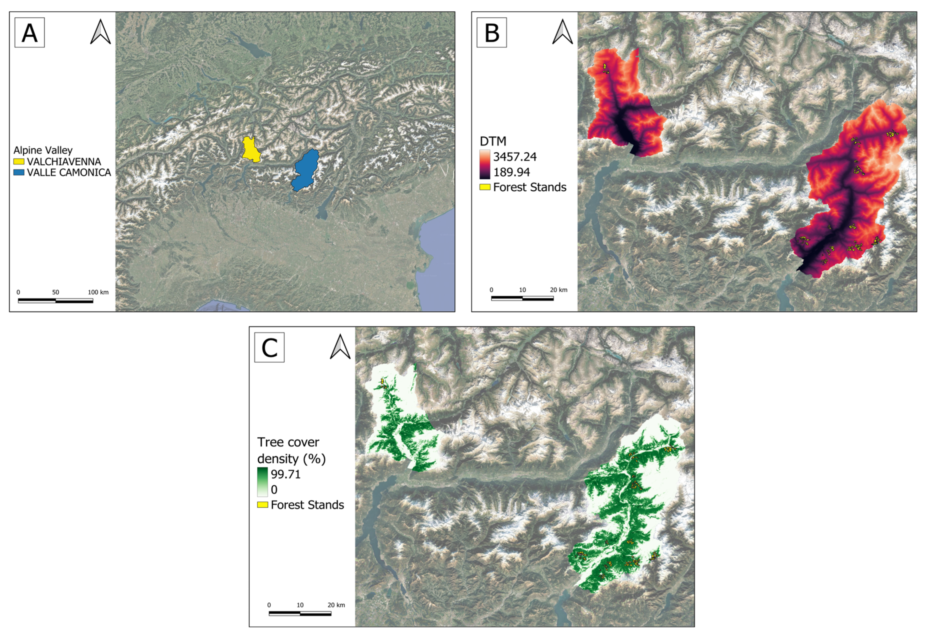
Figure 1. (A) The two study areas in the alpine context; (B) the digital terrain model (DTM, 5 × 5 m resolution) provided by the Lombardy Region geoportal and processed by the authors; (C) the map of tree cover density (Tree Cover Density 2023, raster 10 m/100 m, Europe) derived from the Copernicus Land Monitoring Service and processed by the authors.
Forests 17 00436 g001
Figure 2. Flowchart summarizing the steps for the computation of the structural heterogeneity index (SHI) and the derivation of the PCA structural gradients.
Forests 17 00436 g002
Figure 3. The results of the PCA showing the first two components.
Forests 17 00436 g003
Figure 4. Partial regression plots showing the relationships between the annual increment and (a) the SHI (PC1), (b) the PI (PC2), and (c) the slope as derived from the GLMM. Solid lines indicate model prediction, the shaded areas represent 95% confidence intervals, and tick marks along the x-axis show the distribution of observed data used in the model.
Forests 17 00436 g004
Figure 5. Relative importance of predictors included in the generalized linear mixed model (GLMM) for annual increment. Black bars are the significant ones.
Forests 17 00436 g005
Figure 6. Partial regression plots showing the relationships between timber yield and (a) the SHI (PC1), (b) the PI (PC2), and (c) the elevation, as derived from the GLMM. Solid lines indicate model prediction, the shaded areas represent 95% confidence intervals, and tick marks along the x-axis show the distribution of observed data used in the model.
Forests 17 00436 g006
Figure 7. Relative importance of predictors included in the generalized linear mixed model (GLMM) for timber yield. Black bars are the significant ones.
Forests 17 00436 g007
Figure 8. Partial regression plots showing the relationships between the tourism–recreation value and (a) the SHI (PC1), (b) the PI (PC2), and (c) the slope, as derived from the GLMM. Solid lines indicate model prediction, the shaded areas represent 95% confidence intervals, and tick marks along the x-axis show the distribution of observed data used in the model.
Forests 17 00436 g008
Figure 9. Relative importance of predictors included in the generalized linear mixed model (GLMM) for the tourism–recreation value. Black bars are the significant ones.
Forests 17 00436 g009
Table 2. The PCA loading results of the first two components.
Forest VariablesPC1
(Productive Index)
43.3%
PC2
(Structural Heterogeneity Index)
33.9%
Horizontal diversity index (HDI)−0.1740.717
Tree density (n trees/ha)0.723−0.040
Timber stock (m3/ha)0.6630.305
Stand age (years)−0.0760.625
Disclaimer/Publisher’s Note: The statements, opinions and data contained in all publications are solely those of the individual author(s) and contributor(s) and not of MDPI and/or the editor(s). MDPI and/or the editor(s) disclaim responsibility for any injury to people or property resulting from any ideas, methods, instructions or products referred to in the content.