Article

Spatiotemporal Patterns of Aboveground Carbon Storage in Hainan Mangroves Based on Machine Learning and Multi-Source Remote Sensing Data

1
College of Geographical Sciences, Harbin Normal University, Harbin 150025, China
2
National Key Laboratory for Tropical Crop Breeding, School of Breeding and Multiplication (Sanya Institute of Breeding and Multiplication), Hainan University, Sanya 572025, China
3
Department of Global Agricultural Sciences, Graduate School of Agricultural and Life Sciences, The University of Tokyo, Tokyo 113-8657, Japan
4
Faculty of Agriculture, King Michael I of Romania University of Life Sciences Timisoara, 119 Aradului Avenue, 300645 Timisoara, Romania
*
Author to whom correspondence should be addressed.
These authors contributed equally to this work.
Forests 2026, 17(1), 131; https://doi.org/10.3390/f17010131
Submission received: 24 November 2025 / Revised: 23 December 2025 / Accepted: 17 January 2026 / Published: 19 January 2026

Abstract

As an essential blue carbon ecosystem, mangroves play a vital role in coastal protection, biodiversity conservation, and climate regulation. However, their complex and variable growth environments pose challenges for precise monitoring. Hainan Island represents a region within China where mangrove forests are the most concentrated and diverse in type. In recent years, ecological restoration efforts have led to the recovery of their coverage areas. This study analyzed the spatial distribution, canopy height, and aboveground carbon storage variations in Hainan mangrove forests. Deep-learning and multiple machine-learning algorithms were used to integrate multitemporal Sentinel-2 remote sensing imagery from 2019 to 2023 with unmanned aerial vehicle observations and field survey data. Multi-rule image fusion and deep-learning techniques effectively enhanced mangrove identification accuracy. The mangrove classification achieved an overall accuracy exceeding 90%. The mangrove area in Hainan increased from 3948.83 ha in 2019 to 4304.29 ha in 2023. Gradient-boosted decision tree (GBDT) models estimated average canopy height with a high coefficient of determination (R2 = 0.89), and Random Forest (RF) models yielded the best estimations of total above-ground carbon stock with strong agreement to field observations. Integrating multisource remote sensing data with artificial intelligence algorithms enabled high-precision dynamic monitoring of mangrove distribution, structure, and carbon storage to provide scientific support for the assessment, management, and carbon sink accounting of Hainan mangrove ecosystems.

1. Introduction

Mangroves constitute a distinctive forest wetland ecosystem that inhabits the intertidal zones of tropical and subtropical regions. Characterized by evergreen shrubs or trees of the family Rhizophoraceae as the dominant species, they are distributed along the coastal margins between approximately 30° N and 30° S [1]. With their salt-tolerant root systems and unique physiological adaptation strategies, mangroves play a pivotal role in coastal stabilization and disaster mitigation, habitat provision, water purification, and nutrient interception. They serve as core barriers in maintaining coastal ecological security and biodiversity [2,3,4]. Benefiting from the high productivity and long-term sequestration capacity of organic matter, mangrove forests exhibit substantially higher carbon storage per unit area than terrestrial forests and are regarded as one of the most representative “blue carbon” ecosystems [5]. However, since the mid-20th century, global mangrove forests have undergone considerable decline and degradation due to the combined effects of human activities, such as urban expansion, land reclamation, and overdevelopment, with climate change factors, including sea level rise and intensified extreme events [6,7], posing challenges to the sustainability of coastal socio-ecological systems. Consequently, regional and long-term monitoring of mangrove dynamics, with carbon sink assessments, has become a critical scientific priority for international blue carbon governance and natural ecological restoration.
Remote-sensing technology provides a viable pathway for large-scale, long-term, and repeated observations of mangrove forests. Since the advent of aerial photography and Landsat imagery, mangrove mapping has evolved from early methods of visual interpretation and spectral thresholding to a systematic approach encompassing object-oriented techniques, time-series synthesis, phenological constraints, and multi-source data fusion [8,9,10,11,12,13,14,15,16,17,18], and several baseline datasets have been established at the global/national scale [11,16,18]. Concurrently constrained by cloud cover and tidal inundation, single-source optical imagery frequently exhibits spatiotemporal discontinuities and interclass confusion in tropical coastal scenarios. The all-weather/all-time advantages of synthetic aperture radar (SAR) can partially mitigate these limitations.
Regarding parameter inversion, the acquisition of structural parameters based on high-resolution optical, SAR, and airborne/satellite light detection and ranging (LiDAR) systems has substantially advanced remote sensing estimates of canopy height (CH) and aboveground biomass/carbon storage (AGB/AGC) [19,20,21,22,23,24,25,26,27]; machine learning and deep learning further enhance nonlinear modeling capabilities and classification robustness in complex contexts [28,29,30,31,32,33,34,35,36,37,38,39,40]. Nevertheless, due to the combined effects of tidal phase, cloud cover timing, spectral saturation, and sample representativeness, achieving a balance between temporal stability, classification accuracy, and parameter inversion consistency remains a critical bottleneck for advancing mangrove remote sensing monitoring for operationalization and refinement [30,33,41,42,43,44].
Hainan Island accounts for 20%–30% of China’s mangrove forest area, featuring diverse types and complex coastal morphology, making it an ideal study area for observing restoration outcomes and assessing blue carbon potential. Despite notable restoration achievements in recent years, continuous multiyear quantification of the spatiotemporal distribution dynamics, canopy structure parameters, and aboveground gross carbon (AGC) remains relatively inadequate for Hainan’s mangroves. Integrated remote-sensing frameworks and regional baseline data that simultaneously address distribution mapping, structural inversion, and carbon sink assessments are lacking. This deficiency constrains both the quantification of restoration outcomes and refined management practices, while also affecting the accuracy of blue carbon accounting within the regional carbon neutrality context.
This study used Hainan Island as the research area in response to the aforementioned scientific and practical requirements. Leveraging multi-temporal Sentinel-2 imagery from 2019 to 2023, the study integrated unmanned aerial vehicle (UAV) data with field plot measurements to establish an integrated technical framework comprising ‘multi-rule image synthesis—deep learning mapping—machine learning inversion.’ This approach enables collaborative monitoring and assessment of mangrove distribution, canopy height, and aboveground carbon stocks across a multiyear time series. The primary objectives and contributions of this study were as follows:
  • New pathways in distribution identification: This study proposed a multi-rule image synthesis strategy tailored for intertidal scenarios (including the kernel normalized difference vegetation index (KNDVI)/normalized difference water index (NDWI)/enhanced vegetation index (EVI)/mangrove forest index (MFI) and annual median isoquanti synthesis rules), integrated with the Res-UNet deep-learning algorithm. This approach achieved high-precision mapping of Hainan’s mangrove forests from 2019 to 2023, mitigating the spatiotemporal instability and misclassification issues caused by cloud cover and tidal interference [31,35,37,45].
  • Structure–function parameter coupling inversion: By integrating Sentinel-1/2 spectral, textural, and index features, this study compared the canopy height estimation performance of machine-learning algorithms, including XGBoost, GBDT, and RF. Canopy height was then incorporated as a key feature into AGC inversion, thereby bridging the “structure–function” chain [22,23,26,27,28,36,46,47,48,49,50,51].
  • Empirical constraints and multi-year assessment: By constructing high-quality training and validation samples using UAV and plot-based surveying, this study conducted a synergistic assessment of Hainan’s mangrove area, structure, and carbon stocks from 2019 to 2023. The study quantified the spatiotemporal variation and sources of uncertainty during the restoration period, providing a baseline and methodological framework for regional blue carbon accounting and refined conservation strategies.
  • Scalability for management applications: This study established a technical workflow that combines temporal stability with algorithmic reusability, thereby providing a reference for operational monitoring and cross-regional comparative studies in other mangrove areas across tropical and subtropical regions.
Compared with existing research, the innovation of the current study lies in:
  • Explicitly embedding multi-rule temporal synthesis into deep-learning mapping workflows substantially enhances the stability and accuracy of distribution identification in complex intertidal zones.
  • Using canopy height as a bridge for AGC inversion, the effectiveness of coupling structural and functional information in blue carbon assessment was validated.
  • Providing a comprehensive assessment of the distribution, structure, and carbon storage of Hainan mangrove forests over multiple years through a multi-scale observation loop integrating UAVs, plot surveys, and satellite imagery. This study provides technical support and regional evidence chains for quantifying ecological restoration outcomes and evaluating blue carbon policies.
In recent years, increasing attention has been paid to the application of multi-source remote sensing data and advanced machine-learning techniques for mangrove ecosystem monitoring. Several recent studies published in 2024–2025 have further improved the estimation of mangrove extent, canopy structure, and carbon storage by integrating Sentinel imagery, UAV observations, and data-driven models, highlighting both methodological advances and growing demands for accurate, large-scale mangrove assessments under climate change and coastal development pressures [52,53]. These recent developments underscore the high relevance and timeliness of the present study.
Recent AI-based mangrove studies in Southeast Asia and the Indo-Pacific have widely applied ensemble learning and deep-learning models for mangrove mapping and biomass estimation. However, many of these approaches rely on single-rule temporal compositing and focus on isolated tasks, which remain sensitive to tidal-stage variability in intertidal environments. In this study, we advance existing methodologies by embedding a multi-rule temporal image synthesis strategy into a deep-learning framework specifically designed for intertidal mangroves. In addition, canopy height is introduced as a structural intermediary to strengthen the linkage between remote sensing observations and aboveground carbon estimation at the regional scale.

2. Materials and Methods

2.1. Study Area

The study area is situated on Hainan Island (108°37′–111°03′ E, 18°10′–20°10′ N), within a tropical monsoon climate zone. It covers a total area of approximately 35,400 km2 and has a coastline of approximately 1944 km. The annual mean temperature is 22–26 °C, with annual precipitation of 1000–2600 mm. Rainfall is concentrated between May and October with considerable typhoon impact. The terrain forms an inverted bowl shape with central mountains gradually descending towards the periphery, creating a ring-shaped landscape of mountains, hills, plateaus, and plains. The principal peaks are at Wuzhishan (1867 m) and Yinggeling (1812 m). The principal rivers include the Nandu and Changhua Rivers, which form estuarine wetlands at their mouths and supply mangroves with freshwater, nutrients, and sediment. The soils are predominantly red and coastal saline, suitable for mangrove growth.
Hainan Island is one of China’s most concentrated areas of mangrove distribution, with forests primarily found along the island’s northeastern, southern, and southwestern coasts. The Dongzhaigang Mangrove National Nature Reserve in Haikou City spans approximately 3337 ha, making it China’s first national-level mangrove reserve. The island hosts 26 true mangrove species and 12 semi-mangrove plants, with the dominant species including red mangrove (Rhizophora stylosa), Kandelia obovata, Bruguiera gymnorhiza, Aegiceras corniculatum, and Avicennia marina. Under the influence of tropical–subtropical climatic transitions and typhoon disturbances, the Hainan mangroves exhibit distinct latitudinal distributions and community zonation patterns, performing vital ecological functions in coastal protection, sediment deposition, and water purification. By integrating climatic, topographic, hydrological, and soil conditions, Hainan Island provides an ideal regional foundation for mangrove distribution identification and ecological characterization studies (Figure 1).

2.2. Data Sources

2.2.1. Forest Sample Plot Data

The field and UAV datasets were organized in a hierarchical sampling framework. Field surveys of mangrove forests along the coastal regions of Hainan Island were conducted between April and September 2024, covering typical mangrove distribution areas, including Haikou, Sanya, Dongfang, and Wanning. Correspondingly, field and UAV reference data used in this study were collected in 2024, whereas Sentinel imagery used for canopy height (CH) and aboveground carbon storage (AGC) estimation spanned the period from 2019 to 2023.
In this study, UAV-derived canopy height and field-based carbon measurements collected in 2024 were used to establish the relationships between mangrove structural attributes and multi-source remote sensing features. These structural–spectral relationships were assumed to be temporally stable over the short study period, allowing the trained models to be applied retrospectively to Sentinel imagery from 2019 to 2023.
Given that mangrove canopy height and aboveground carbon typically change gradually over multi-year timescales at the regional scale, this retrospective application (backcasting) is unlikely to introduce substantial bias in the estimation of spatial patterns and temporal trends. In practice, Sentinel imagery from 2023 represents the closest temporal match to the 2024 field observations and serves as the effective baseline for model calibration, while estimates for earlier years (2019–2022) reflect relative temporal changes propagated backward from this reference state.
To ensure data representativeness, the surveyed areas encompassed both naturally occurring and disturbed secondary mangrove forests. Plot coordinates were recorded using Garmin GPSMAP 63csx handheld GPS (Google Inc., Menlo Park, CA, USA) and Google Earth tools. Ten survey areas were established: five for model training (64 ground plots, each covering a 10 m × 10 m area, used for aboveground carbon measurements and model calibration) and five for accuracy validation. In total, 7660 mangrove and non-mangrove samples were collected.
To acquire high-precision canopy structure information, an aerial survey was conducted using a DJI Mavic 3M drone (DJI, Shenzhen, China) under clear, windless conditions at multiple viewing angles. The flight altitude was set at 20–30 m, with forward and sideways overlap rates of 70% and 80%, respectively, and an image resolution of 10 cm. The images were processed using motion recovery algorithms to generate a digital surface model (DSM), which was then combined with the terrain data to construct a digital elevation model (DEM). The bare-earth DEM was generated by filtering ground points from the UAV-derived point cloud using a semi-automated classification approach implemented in LiDAR360, followed by manual correction to remove residual vegetation points. Ground point identification was assisted by low-tide acquisition conditions and visual interpretation to ensure the extraction of the lowest elevation surface. The differences between these models were used to calculate canopy height (CH). Three-dimensional reconstruction and point cloud processing were performed using DJI Terra and LiDAR360 V8.0 software (Beijing Digital Green Soil Technology Co., Ltd., Beijing, China), respectively. Ground points were extracted using semi-automated classification and manual correction to ensure the accuracy of the DEM. The final average canopy height was aggregated to a 10 m × 10 m grid, yielding data from over 6000 spatial sample plots, which were used exclusively for canopy height model training and validation. UAV-derived canopy height was evaluated against field-measured tree heights collected in representative plots. The comparison showed a strong agreement, with a small mean bias (<0.5 m) and a low RMSE (<1.0 m), indicating that UAV-derived canopy height can be regarded as a reliable reference for subsequent satellite-based modeling. Therefore, UAV-derived canopy height was treated as reference canopy height in this study.
In representative plots, standard trees were selected for the aboveground carbon storage assessment. In this study, aboveground carbon storage refers exclusively to shoot biomass (stems, branches, and foliage), and belowground biomass was not considered. Each plot covered 100 m2 (10 m × 10 m), and tree species composition and abundance were surveyed. Three to five healthy individuals with a diameter at breast height exceeding 5 cm and no apparent disease were selected. Tree height and diameter at breast height (DBH) were measured in the field.
Aboveground biomass was estimated using species-specific or regionally applicable allometric equations relating DBH and tree height to shoot biomass, as reported in previous studies on Chinese mangroves [54]. In this study, aboveground biomass refers exclusively to shoot biomass (stems, branches, and foliage), and belowground biomass was not considered.
Three-dimensional laser scanning of the trunk and foliage of the sampled trees determined the volume proportions of the specimens collected for laboratory analysis. Samples were oven-dried at 70 °C to constant weight, then incinerated at 550 °C to determine ash mass. Carbon content was calculated using the following formula:
C = f × ( W d r y W a s h )
where C is the carbon content (g), W d r y is the oven-dried mass of the sample (g), W a s h is the ash mass after combustion (g), and f is the carbon fraction. In this study, a carbon fraction of f = 0.5 was applied for aboveground carbon estimation. A carbon fraction of 0.5 was adopted to convert dry biomass to carbon mass, following common practice in forest carbon studies.

2.2.2. Remote Sensing Data

  • Google Earth imagery integrates data from multiple satellite and aerial sources, including WorldView, GeoEye-1, and QuickBird, achieving spatial resolutions as high as 0.3 m. It delivers sub-meter spatial accuracy and 16-bit radiometric resolution [55]. The imagery underwent geometric correction, orthorectification, and atmospheric radiation correction by using the WGS_1984_Web_Mercator projection (EPSG:3857) with a planar positioning error of less than 2 pixels. This study used multitemporal cloud-free imagery (average cloud cover < 5%) covering the mangrove distribution areas on Hainan Island from 2019 to 2023 for precise mangrove boundary identification and manual feature verification. Although this dataset offers high spatial resolution, its spectral range is limited to the visible band. Consequently, multispectral data must be integrated to supplement vegetation index and cover estimation.
  • The Sentinel-1 series constitutes a vital component of the European Space Agency’s Copernicus program and comprises the twin-satellite systems Sentinel-1A and Sentinel-1B, which possess all-weather and all-time observation capabilities. This study utilizes vertical–vertical (VV) and vertical–horizontal (VH) dual-polarization data acquired in the Interferometric Wide Swath (IW) mode, featuring a spatial resolution of 5 m × 20 m and a swath width of 250 km. Following the decommissioning of Sentinel-1B in 2021, the data acquired after 2023 were obtained solely from Sentinel-1A. Using the Google Earth Engine (GEE) platform, the COPERNICUS/S1_GRD dataset covering the Hainan mangrove area from 2018 to 2023 was acquired. A Level-1 pre-processing workflow was executed, which encompassed thermal noise removal, radiometric calibration, and geometric correction. All data were resampled to a 10 m resolution in the WGS84 projection (EPSG:4326). Subsequently, a −30 dB threshold filter and mask function were applied to eliminate pixels with low signal-to-noise ratio. The spatiotemporal mean composite images were then calculated based on the VV/VH polarization bands. To reduce short-term environmental variability, including tidal fluctuations in intertidal mangrove environments, multi-temporal Sentinel-1 composites were constructed using all available observations within each year. This compositing strategy helps to average radar backscatter responses across different tidal stages, thereby reducing the influence of extreme low- or high-tide conditions on individual acquisitions. This process ultimately generated a 128-scene SAR composite image covering the potential distribution zone of the Hainan mangrove forests, thereby providing scattering characteristic information for subsequent canopy structure inversion.
  • The Sentinel-2 twin-satellite system comprises Sentinel-2A (launched in June 2015) and Sentinel-2B (launched in March 2017), each equipped with a multispectral imager (MSI). This instrument features 13 spectral bands (443–2190 nm) covering the visible light, red-edge, near-infrared, and shortwave-infrared regions, with a revisit period of 5 d. The red-edge bands (B5–B8A) exhibited high sensitivity to chlorophyll content variations, whereas the shortwave infrared bands (B11 and B12) were suitable for canopy structure and water content inversion. This study used Level-2A surface reflectance products (COPERNICUS/S2_SR_HARMONIZED) that underwent atmospheric correction and orthorectification via the Sen2Cor algorithm. The reflectance values ranged from 0 to 1, with coordinates in the WGS84 coordinate system. On the GEE platform, imagery with a cloud cover < 30% from 2018 to 2023 was selected. The cloud-contaminated pixels were removed using a QA60 band cloud mask. To ensure spatial consistency, the 20 m bands (B5–B8A, B11, B12) were resampled to a 10 m resolution using nearest neighbor interpolation, aligning them with the 10 m bands (B2–B4, B8). Annual cloud-free reflectance images were generated using the median composite method. Similar to the Sentinel-1 processing, these indices were generated from multi-temporal image composites rather than single-date observations, which helps to mitigate variability introduced by different tidal stages in intertidal mangrove environments. Subsequently, 11 bands were stacked within the ENVI 5.6 software to compute 17 vegetation indices (including NDVI, SAVI, MSAVI, MTCI) and 88 texture features based on the grey-level co-occurrence matrix (GLCM) (including mean, contrast, entropy, correlation). This yielded a high-dimensional, multi-source dataset comprising 116 features that provided input variables for mangrove distribution identification, canopy height inversion, and carbon stock estimation (Table 1).

2.3. Methods

2.3.1. Multi-Rule Synthesis Method for Remote Sensing Images

This study conducted remote-sensing image preprocessing and analysis on the Google Earth Engine (GEE) cloud platform to ensure computational consistency and data reproducibility. The qualityMosaic function was used to perform quality selection and spatiotemporal consistency optimization on the multitemporal imagery based on a single-rule optimal pixel mosaicking method. During image mosaicking, four spectral indices were incorporated: kernel normalized difference vegetation index (KNDVI), enhanced vegetation index (EVI), normalized difference water index (NDWI), and mangrove forest index (MFI). These indices extracted ecological information pertaining to vegetation vigor, water body distribution, and intertidal zone characteristics (Table 2). Specifically, KNDVI enhanced sensitivity to vegetation changes, EVI performed better in areas of high vegetation cover, NDWI was used to identify water body boundaries, and MFI aided in detecting periodically inundated mangroves in intertidal zones.
By using a dual-rule synthesis method based on the maximum index value and median of the time series, the impact of seasonal fluctuations and extreme values on image quality was effectively mitigated. This enhanced spectral stability and spatial consistency, thereby providing high-quality input features for subsequent deep-learning applications. The resulting multi-index fusion imagery enabled the multi-dimensional characterization of mangrove ecosystems, furnishing deep-learning models with richer spectral and structural information.
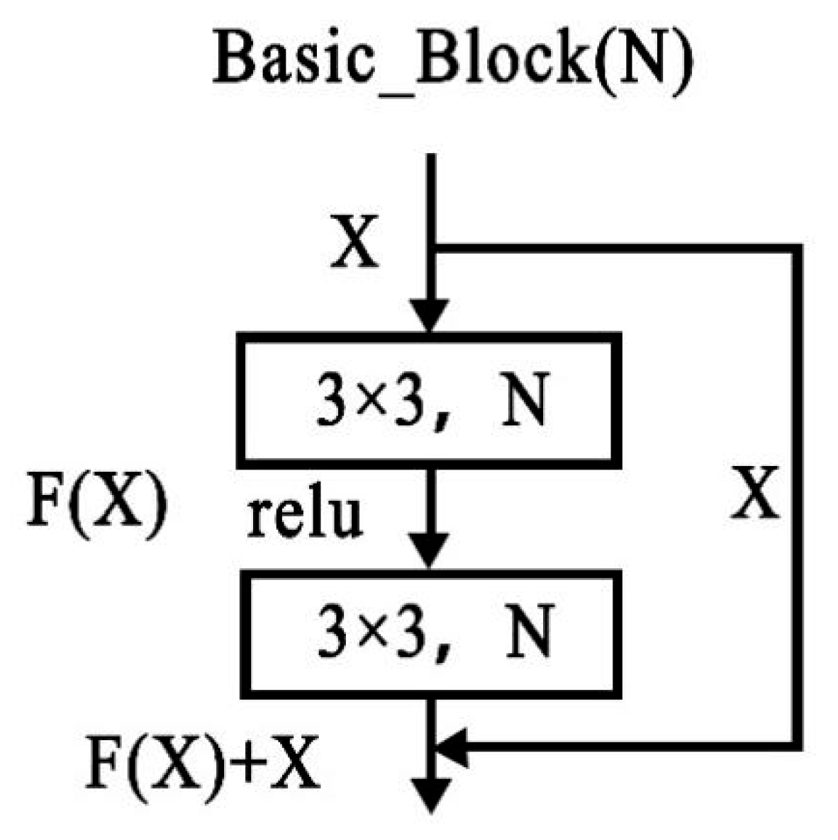
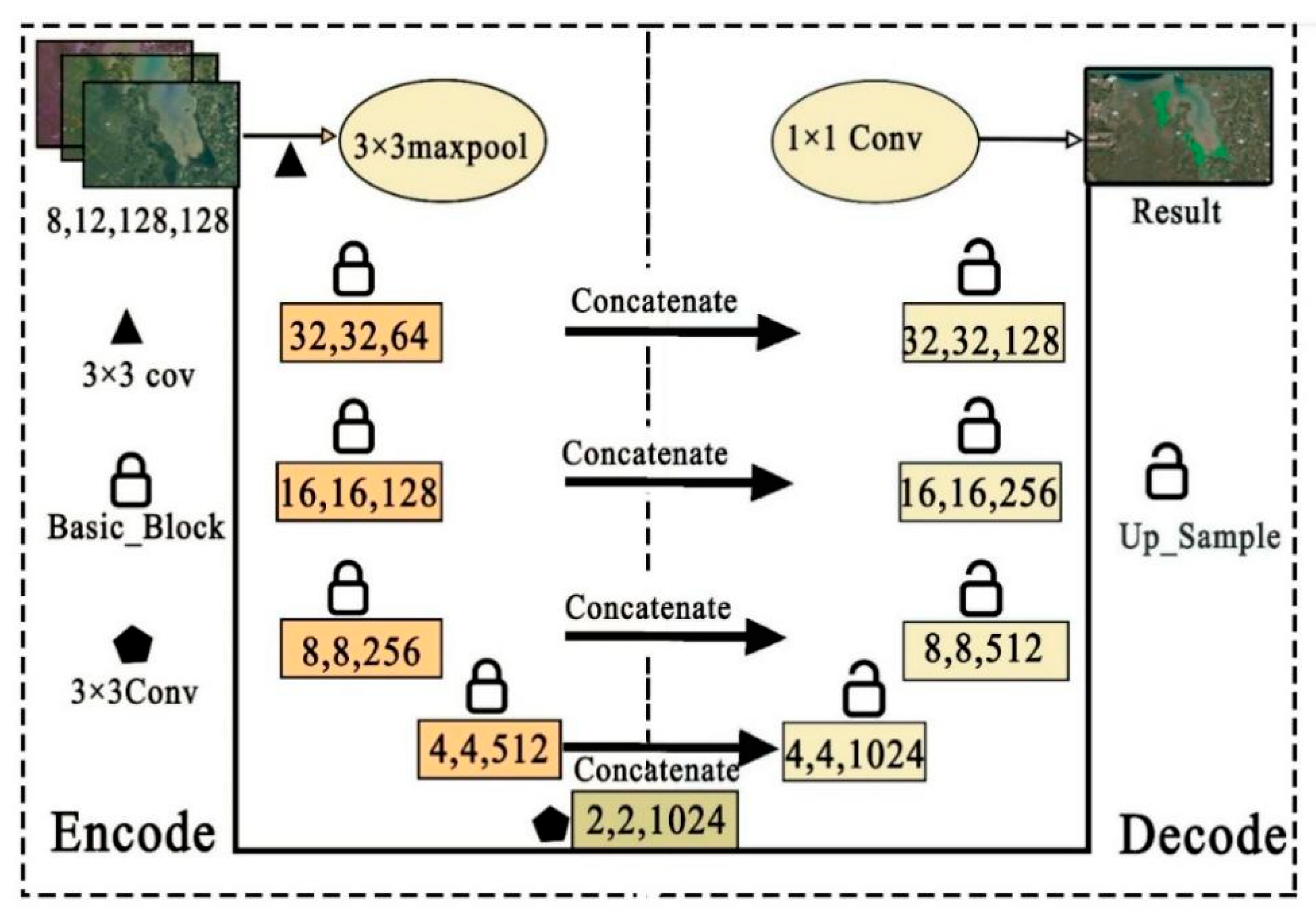
We constructed a ResNet34–UNet deep-learning model to identify mangrove distribution, while a deep residual network (ResNet) served as the primary feature-extraction backbone. Its residual learning mechanism mitigates the vanishing gradient problem, enabling effective extraction of deep spectral and spatial features from remote sensing imagery. The U-Net architecture uses skip connections during the decoding phase to fuse multiscale features, thereby enhancing spatial and semantic accuracy in pixel-level classification. The model was implemented within the TensorFlow framework using the Adam optimizer for parameter updates. It incorporates mixed-up data augmentation alongside a weighted cross-entropy loss function to address class imbalance and bolster model generalization capabilities. The model architecture and optimization strategy are illustrated in Figure 2 and Figure 3.
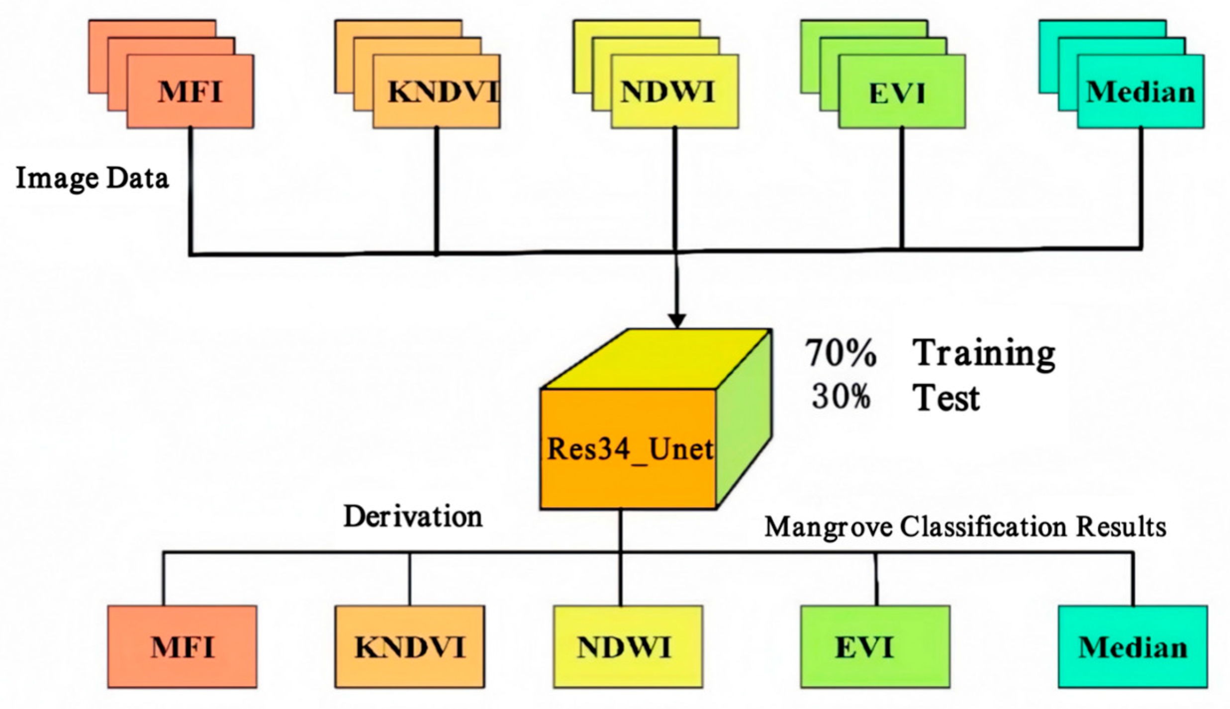
To enhance the accuracy of mangrove classification, this study implemented a deep-learning-based classification approach combined with a multi-rule remote sensing image compositing strategy, following previously reported methods. Multiple compositing rules, including maximum KNDVI (MAX-KNDVI), maximum EVI (MAX-EVI), maximum NDWI (MAX-NDWI), maximum MFI (MAX-MFI), and the median rule, were used to generate complementary image representations that characterize different ecological conditions of mangrove forests.
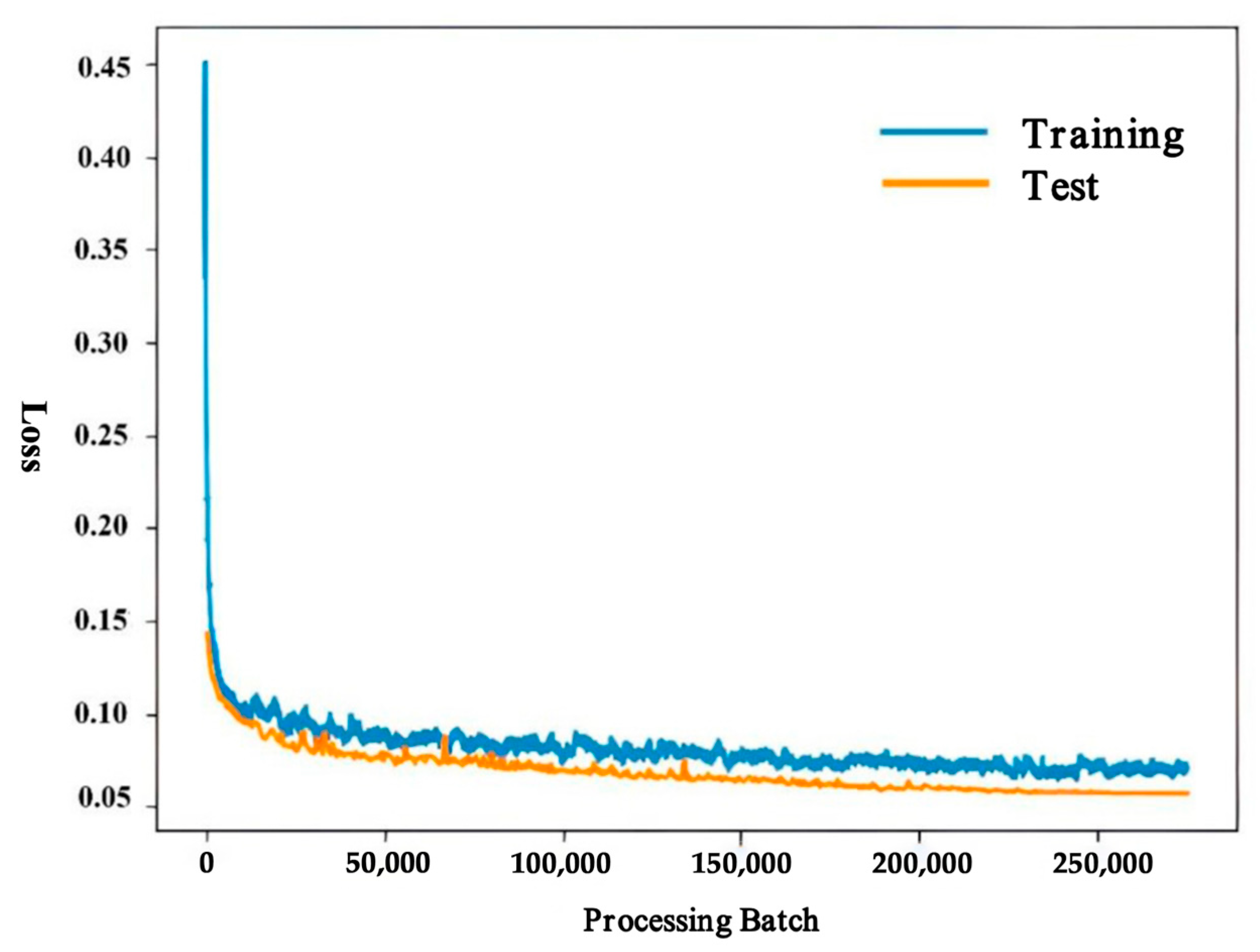
All composited images were generated from multi-temporal Sentinel-2 observations after cloud masking and radiometric correction and were stacked as multi-channel inputs to the deep-learning model to achieve feature-level data fusion. Training samples were validated using high-resolution Google imagery and field survey data to ensure labeling accuracy. The dataset was divided into training and testing subsets at a ratio of 7:3 to ensure model stability and reliable performance evaluation. Internal and external validation strategies were adopted to evaluate the recognition accuracy of the deep-learning-based model. Model training was implemented using the PyTorch 2.0 framework on a hardware environment comprising an Intel i9-13900HX CPU (Intel Corporation, Santa Clara, California, USA) (24 cores and 32 threads, up to 5.40 GHz) and an NVIDIA RTX 4060 GPU with 8 GB of graphics memory. During training, the variation in the cross-entropy loss function was monitored to assess model convergence, as illustrated in Figure 4. The loss curve indicates that the model achieved stable convergence after approximately 100,000 iterations. The overall workflow of the multi-rule compositing and deep-learning classification process is illustrated in Figure 5.

2.3.2. Estimation of Mangrove Canopy Height and Aboveground Carbon Storage

To estimate canopy height and aboveground carbon storage (AGC) in Hainan’s mangrove forests, this study integrated Sentinel-1 SAR, Sentinel-2 multispectral, and ground-based plot survey data to estimate the canopy height and AGC in Hainan’s mangrove forests. The research workflow comprised four stages: feature extraction, feature selection, model construction, and validation.
The input features encompassed 11 Sentinel-2 spectral bands, 17 vegetation indices (such as NDVI and EVI), 88 texture features based on the grey-level co-occurrence matrix (GLCM), and the VV and VH polarization backscatter coefficients from Sentinel-1. These features characterize mangrove ecological traits across multiple dimensions, including spectral, structural, and microwave responses. To mitigate redundant information and collinearity interference, Pearson correlation coefficients were first calculated between each feature and the target variable. The Pearson correlation quantifies the linear relationship between two variables; a higher absolute value indicates a stronger influence of that feature on the target variable. Highly collinear features were then filtered out using a variance inflation factor (VIF) analysis (VIF < 10) to ensure independence of the input variables and model robustness.
The modeling phase used three ensemble learning algorithms: extreme gradient boosting (XGBoost), gradient boosting decision trees (GBDT), and random forests (RF). XGBoost is a scalable gradient boosting framework that optimizes model complexity and computational efficiency through regularization terms and second-order gradient-based tree splitting strategies [56]. The GBDT algorithm constructs an additive ensemble of decision trees by iteratively fitting residuals, thereby progressively improving predictive accuracy [57], and the RF model enhances robustness and reduces overfitting through bootstrap sampling and ensemble averaging across multiple decorrelated decision trees [58]. All models were constructed using the Python 3.8.19 environment (PyCharm 2020.1, Prague, Czech Republic), with key hyperparameters (including learning rate, tree depth, sample proportion, and L2 regularization coefficient) optimized through grid search and 10-fold cross-validation.
The model performance was assessed using the coefficient of determination (R2), root mean square error (RMSE), and mean absolute error (MAE). The model demonstrating optimal performance was ultimately used to generate spatial distribution results for the Hainan mangrove canopy height and aboveground carbon storage from 2019 to 2023.

3. Results

3.1. Distribution Range of Mangroves in Hainan

3.1.1. Results of Mangrove Distribution Identification in Hainan

The multi-rule remote sensing image synthesis and deep learning model (MR_DLM_2020) was used to identify the spatial distribution range of Hainan mangrove forests from 2019 to 2023. This model integrated Sentinel-1 radar data with Sentinel-2 multispectral data and combined multiple spectral indices (KNDVI, EVI, NDWI, MFI, median rule) to achieve a detailed characterization of mangrove distribution. Different image synthesis methods exhibited variations in mangrove distribution. Of these, the median synthesis method demonstrated optimal performance in mitigating cloud interference and enhancing image consistency, thereby providing high-quality input data for subsequent classification.
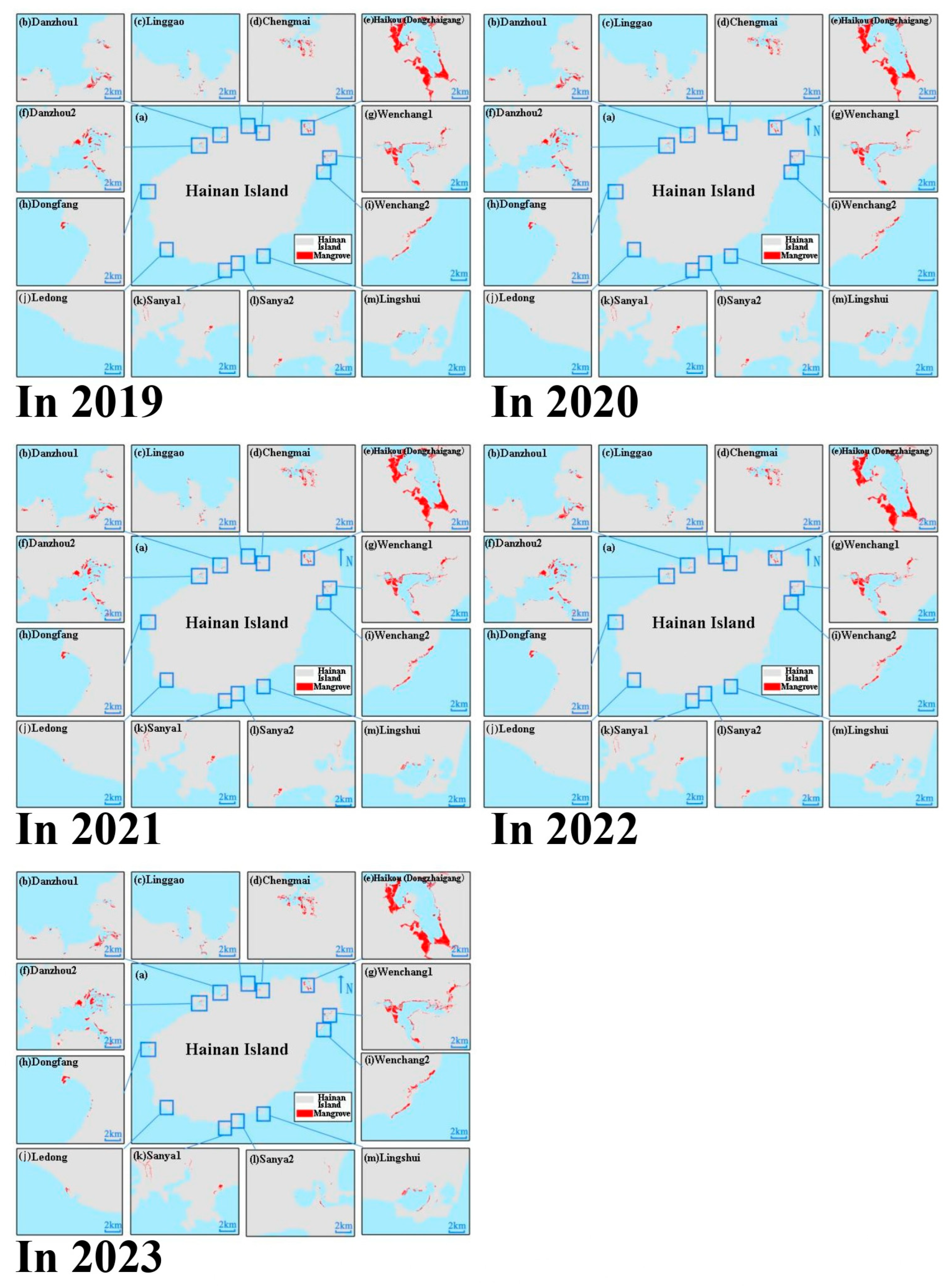
Spatial identification results indicated that Hainan’s mangrove forests were primarily distributed across coastal intertidal zones in Haikou, Wenchang, Danzhou, Dongfang, Ledong, and Sanya, exhibiting a typical ‘estuary–bay–lagoon’ zonal distribution pattern (Figure 6). Of these, Dongzhai Harbor, Qinglan Bay, Xincun Bay, and Yingge Bay constituted concentrated mangrove areas with relatively intact ecosystems. In contrast, the mangrove distribution in the northwestern coastal regions (such as Lingao and Danzhou) is more fragmented and often intermingled with artificial aquaculture ponds. Overall, the mangrove distribution in Hainan exhibited a spatial pattern characterized by eastern concentration, southern sparseness, and western stability.

3.1.2. Model Accuracy Validation and Result Evaluation

The internal validation results (Table 3) indicate that the precision, recall, and F1-score for the mangrove category were 0.92, 0.89, and 0.91, respectively, and the corresponding values for the non-mangrove category were 0.98, 0.99, and 0.99, respectively. These findings demonstrated the high accuracy of the model for mangrove identification and its superior precision in distinguishing non-mangrove areas. The external validation comparisons are presented in Appendix A (Table A1) and Table 4. MR_DLM_2020 outperformed the existing datasets (HGMF_2020, GMW_V3.0_2020, LREIS_V2_2020) in terms of overall precision (90%) and kappa coefficient (80%). In particular, under the median rule, the producer accuracy for mangroves reached 94.6%, with a user accuracy of 85.1%, substantially surpassing the other rules.
The MR_2020_Median model demonstrated superior performance in mangrove spatial identification and accurately reflected mangrove boundaries and spatial continuity. Further validation using drone aerial imagery confirmed that the mangrove distribution inferred by the MR_DLM_2020 model aligned closely with the actual mangrove areas, successfully identifying newly formed mangroves that were not covered by existing datasets. This outcome demonstrates the robust generalization capability and environmental adaptability of the model, rendering it suitable for the high-precision remote-sensing monitoring of mangroves.

3.1.3. Analysis of Distribution Patterns in Mangrove Forests

Based on the inference results from the MR_DLM_2020 model, the Hainan mangrove forests tended to increase between 2019 and 2023 (Table 5). The total mangrove area across the province increased from 3948.83 ha in 2019 to 4304.29 ha in 2023, representing a growth rate of 9.0%. Of these, Wenchang City recorded the most marked increase (from 947.21 ha to 1083.83 ha), followed by Lingshui County (from 44.8 ha to 94.97 ha) and Sanya City (from 78.27 ha to 107.39 ha). Haikou City consistently maintained the largest mangrove area in the province (1775.08–1817.85 ha), sustaining a steady expansion. Dongfang City and Lingao County experienced minor fluctuations in mangrove coverage between 2022 and 2023, which were primarily attributed to coastal development and natural disturbances. The eastern coastline (Wenchang, Qionghai) witnessed marked expansion driven by both natural regeneration and artificial replanting, the southern region (Sanya, Lingshui) experienced substantial mangrove fragmentation due to coastal construction and tourism activities, and the western area (Dongfang, Ledong) maintained a growth trajectory propelled by ecological restoration projects. To facilitate comparison among regions with different baseline mangrove extents, the relative percentage growth of mangrove area was additionally calculated for each municipality. When expressed as percent change, some regions with smaller initial mangrove areas exhibited higher relative growth rates despite smaller absolute increases. The results indicate that Hainan’s mangrove ecological restoration and conservation policies have yielded considerable outcomes, with mangrove ecosystems demonstrating a clear trajectory towards recovery. The MR_DLM_2020 model exhibited robust stability and reliability in dynamically monitoring mangrove areas and spatial changes, providing a scientific basis for coastal ecological conservation and blue carbon assessment in Hainan Province.

3.2. Accuracy Verification Results

3.2.1. Validation Results for Canopy Height Modeling Accuracy

To evaluate the performance of different machine-learning algorithms in estimating mangrove canopy height, this study constructed three models: random forest (RF), extreme gradient boosting tree (XGBoost), and gradient boosting decision tree (GBDT). Cross-validation was conducted using independent sample points. The model accuracy was comprehensively assessed using the coefficient of determination (R2), root mean square error (RMSE), and relative root mean square error (RRMSE).
All three models achieved high-precision canopy height inversion, although their performances exhibited notable differences (Table 6). Among them, the GBDT model performed best, with an R2 of 0.89, RMSE of 1.39 m, and RRMSE of 0.39. The XGBoost model ranked second (R2 = 0.85), and the RF model showed lower performance (R2 = 0.82). The superior estimation performance of the GBDT model stems primarily from its efficient fitting capability for nonlinear relationships among the multisource remote sensing features. This suppresses noise effects and enhances the overall generalization ability when simultaneously integrating spectral, radar, and textural features. Although the RMSE magnitude exceeds the reported multi-year mean canopy height change (0.58 m), the model is primarily intended to characterize spatial variability in canopy height rather than detect subtle interannual changes at the pixel level. To account for sampling uncertainty, the robustness of model performance was evaluated using repeated cross-validation; however, confidence intervals for R2 were not explicitly reported due to the limited sample size (n = 64). This limitation is further discussed in Section 4.
The results of the feature importance analysis elucidated the sources of variation in the model accuracy. The red-edge bands (B5–B8A), shortwave infrared bands (B11 and B12), and grey-level co-occurrence matrix (GLCM) texture indices contributed most to canopy height estimation, indicating a close coupling between canopy structure and spectral reflectance characteristics. Overall, the GBDT model demonstrated marked advantages in handling complex terrain features and provided reliable technical support for subsequent studies on mangrove vertical structures.

3.2.2. Validation Results for Aboveground Carbon Storage Modeling Accuracy

Building on the canopy height inversion results, this study constructed three models—RF, GBDT, and XGBoost—using canopy height, multispectral bands, vegetation indices, and textural features as input variables. These models were used to compare and validate the accuracy of above-ground carbon storage (AGC) in the Hainan mangroves. A similar model evaluation was conducted using the R2, RMSE, and RRMSE metrics. The results indicate that all three models demonstrated satisfactory fitting performance (Table 7). Of them, the RF model exhibited the best overall performance, with an R2 of 0.67, RMSE of 17.33 MgC, and RRMSE of 0.34. The GBDT model ranked second (R2 = 0.63), whereas the XGBoost model performed slightly poorer (R2 = 0.61). The RF model demonstrated stable performance under multiple feature inputs, effectively handling nonlinear relationships between variables and noise interference, thereby exhibiting a high generalization capability.
Feature importance analysis indicated that canopy height was the most important explanatory variable in aboveground carbon Storage estimation, followed by the B8 (near-infrared) and B11 (shortwave infrared) bands, with spectral indices, such as ARVI and MTCI. These variables reflect the combined variations in the mangrove canopy leaf area index, chlorophyll content, and biomass, which play pivotal roles in carbon stock estimation. Furthermore, texture features such as B9_SEC and B12_IOM contribute to the characterization of canopy structural complexity, thereby enhancing the overall accuracy of the model.
Overall, the RF model demonstrated optimal robustness and reliability in estimating terrestrial carbon stocks, providing a solid modeling foundation for subsequent research on the spatiotemporal dynamics of carbon sinks in Hainan’s mangrove forests.

3.3. Changes in Canopy Height of Hainan Mangroves, 2019–2023

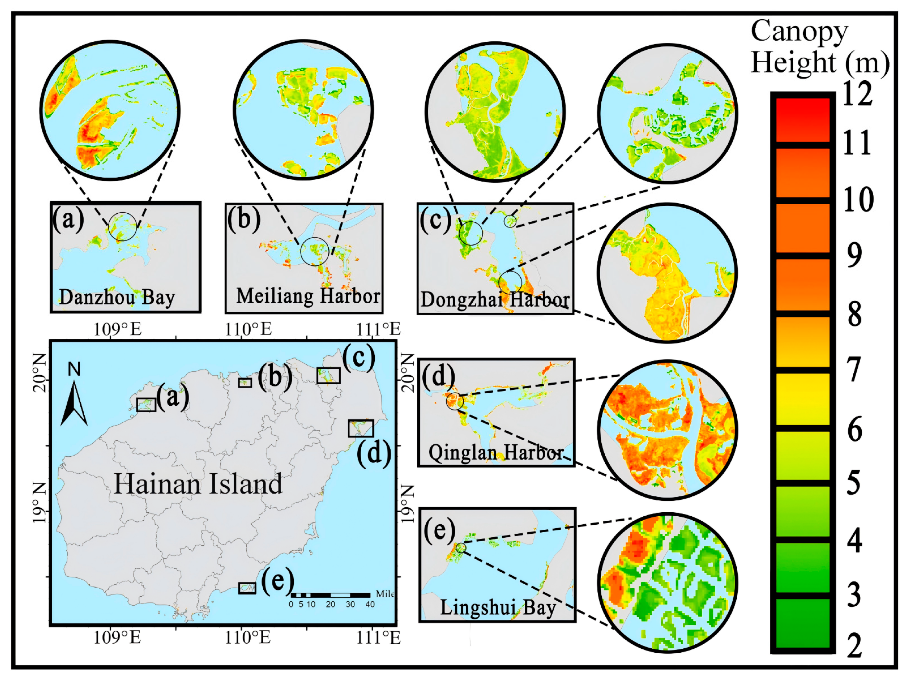
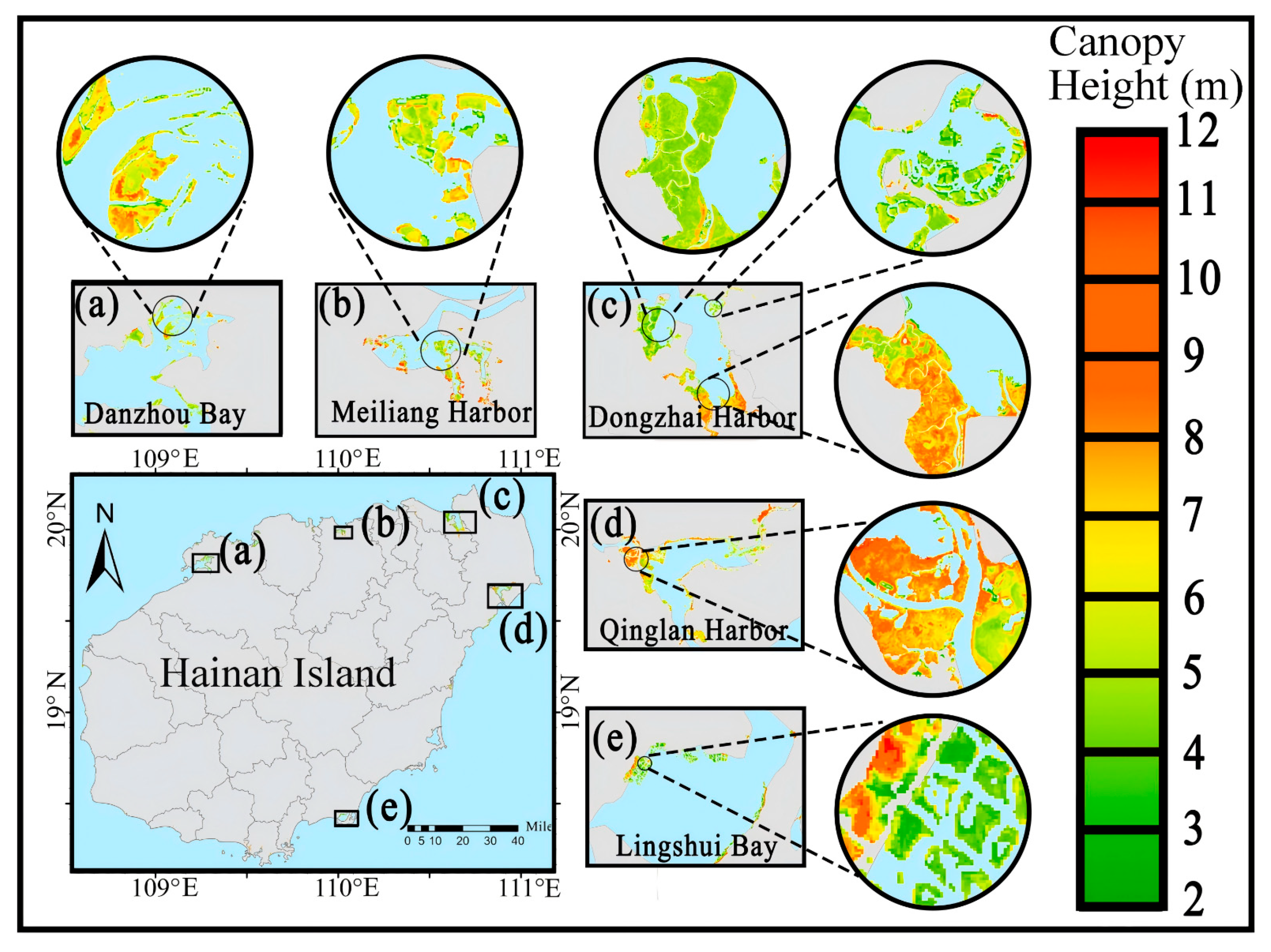
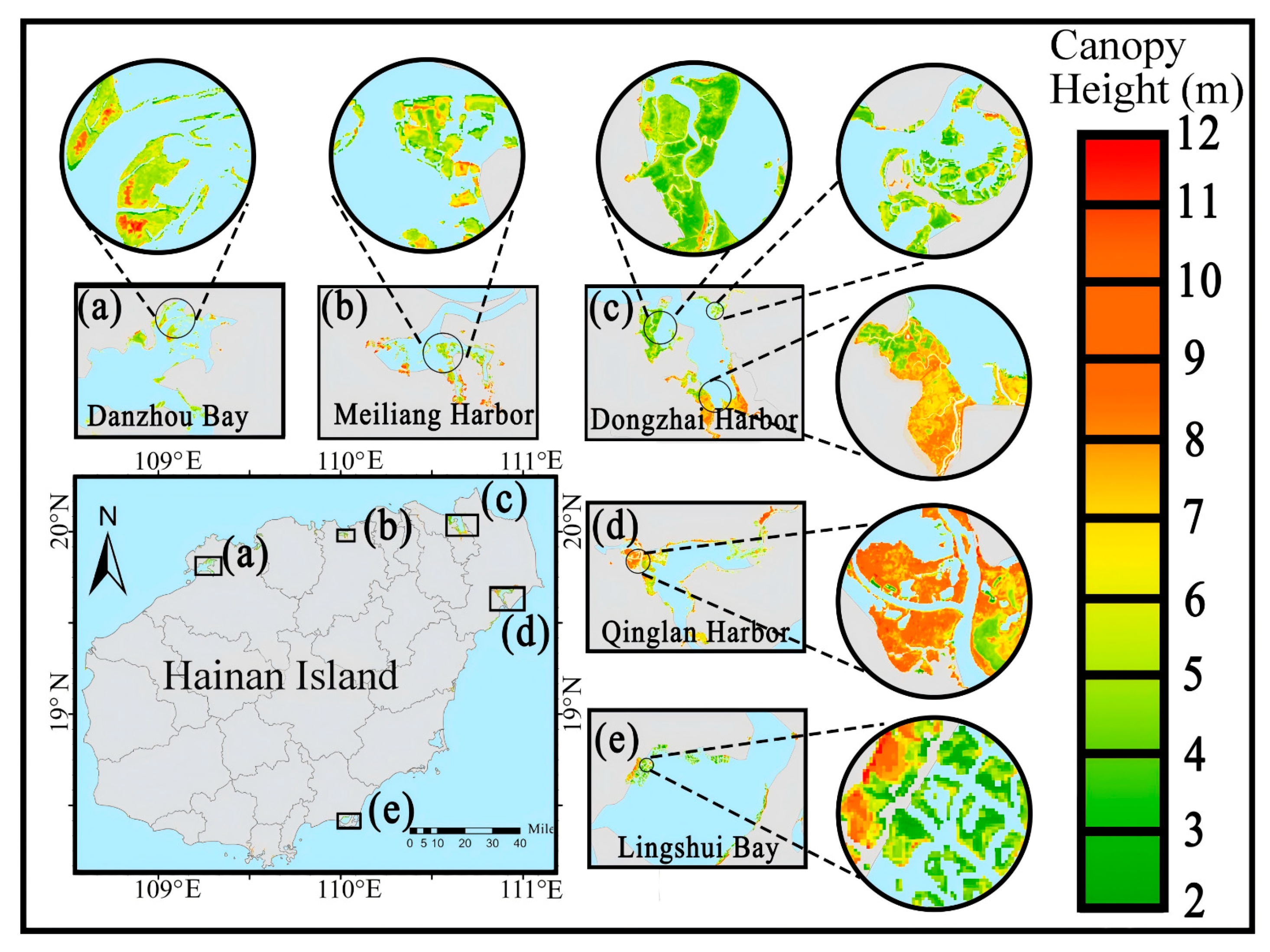
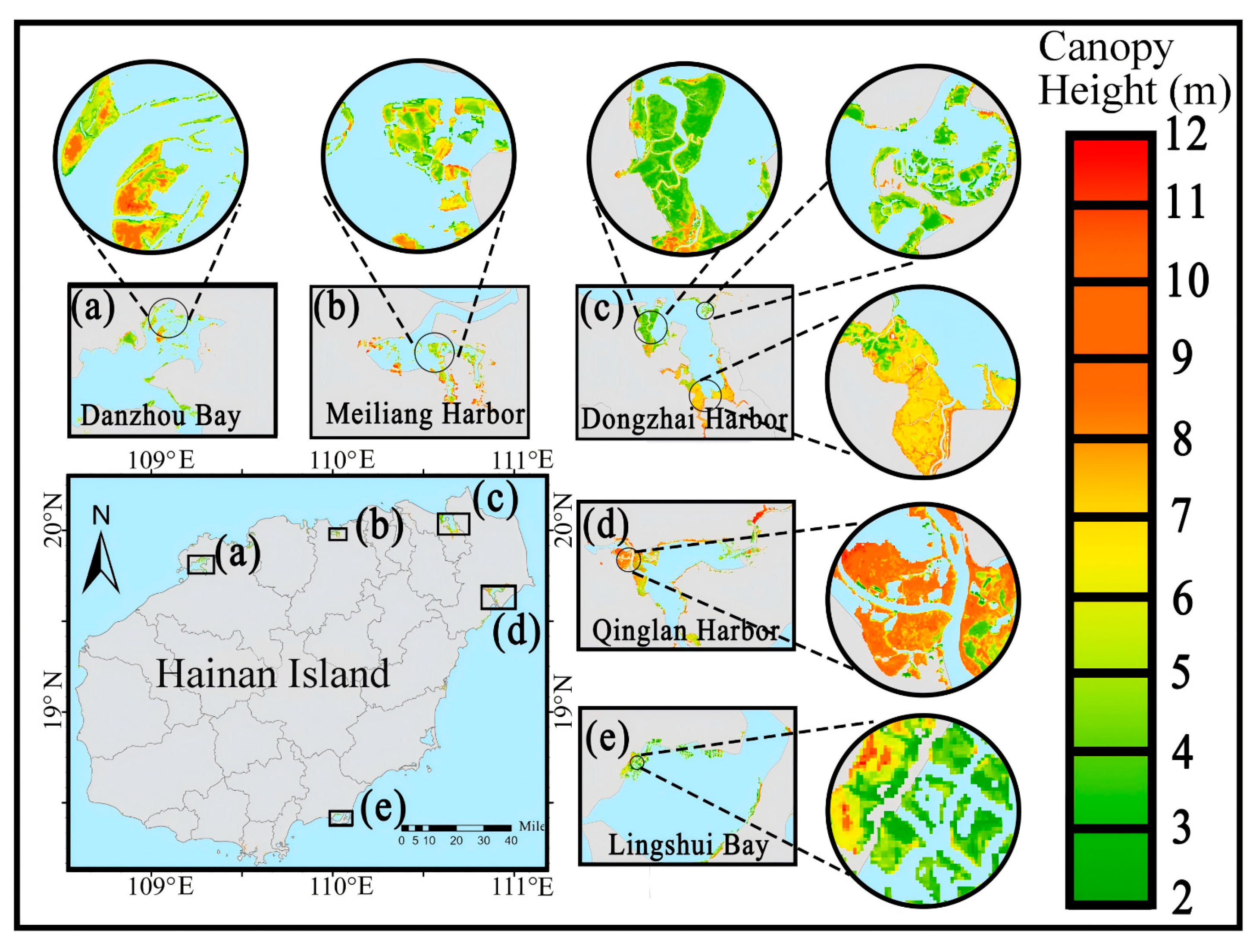
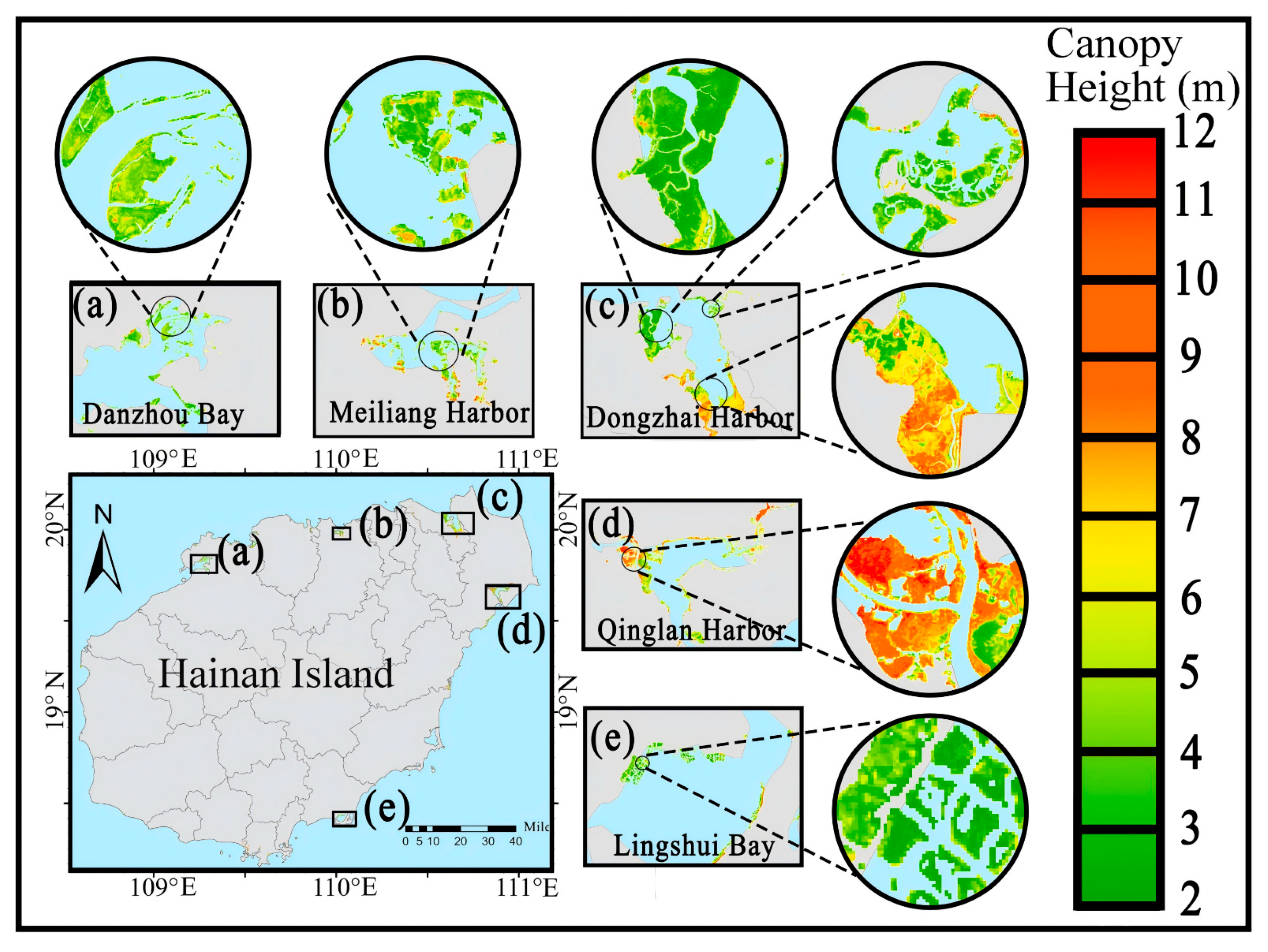
Based on the GBDT model estimation results, the canopy height of Hainan’s mangrove forests overall showed an upward trend followed by a slight decline between 2019 and 2023. Spatially, areas with high canopy heights were concentrated in coastal zones, such as Dongzhai Harbor, Qinglan Harbor in Wenchang, and Qionghai. These regions feature mature mangrove community structures, older stands, and favorable site conditions, demonstrating strong vertical growth potential. In contrast, areas such as Dongfang, Lingao, and Ledong generally exhibited lower canopy heights and were predominantly distributed in disturbed or early-stage recovery zones. This indicates that their ecosystems remained in the process of restoration and reconstruction (Figure 7, Figure 8, Figure 9, Figure 10 and Figure 11).
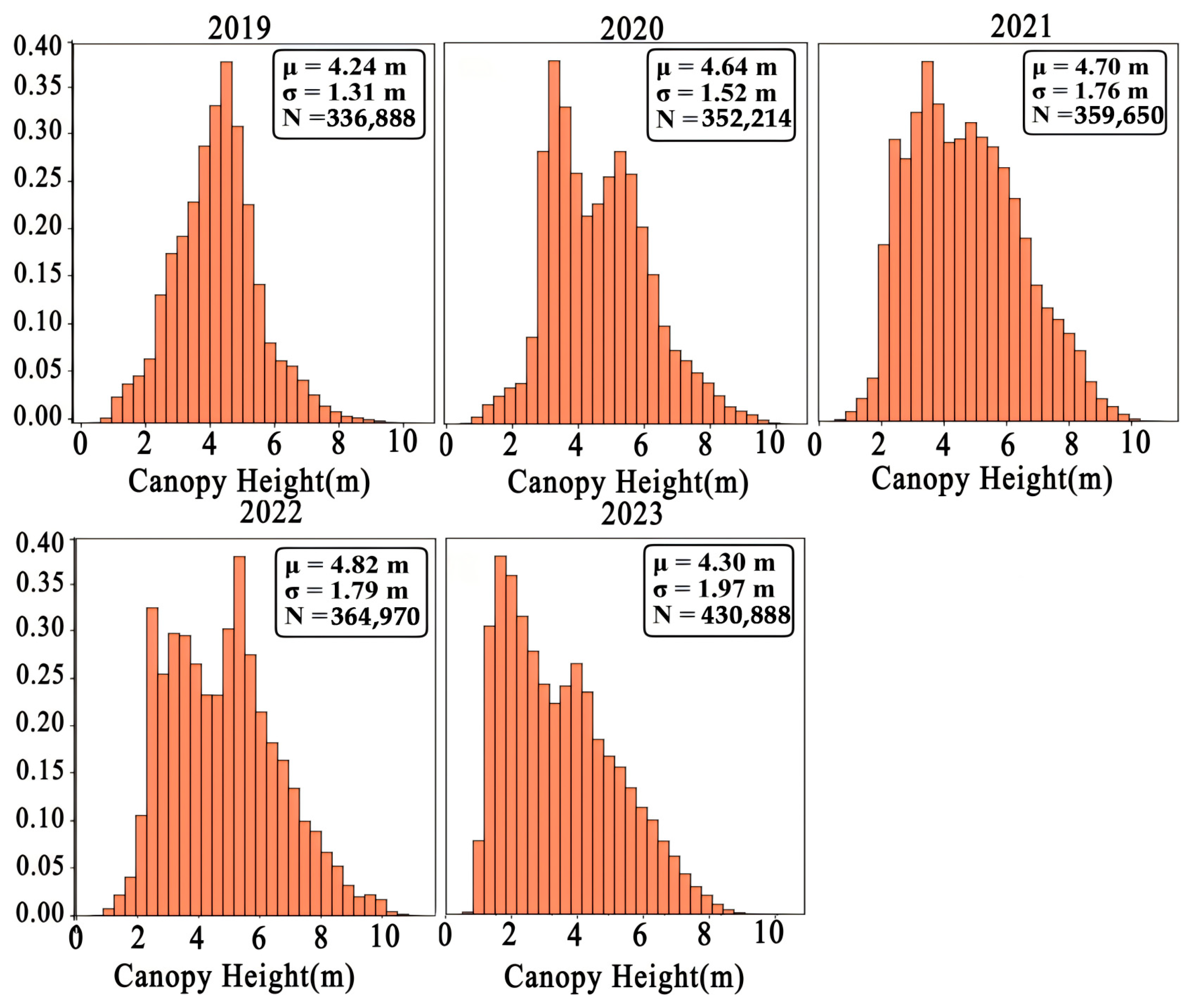
Based on the arithmetic mean, the average canopy height increased from 4.24 m in 2019 to 4.82 m in 2022 before declining slightly to 4.30 m in 2023. However, considering the skewed distribution of canopy height (Figure 12), the median canopy height exhibited a more stable temporal pattern, suggesting that the apparent decline in 2023 is mainly driven by a limited number of low-height pixels rather than a generalized reduction in canopy structure. Between 2019 and 2021, the distribution of mangrove canopy height was relatively concentrated and exhibited an approximately normal distribution, indicating a stable mangrove ecosystem structure. From 2022 onwards, the canopy height distribution shifted markedly to the right with an increased standard deviation (from 1.31 m to 1.79 m), reflecting heightened spatial heterogeneity. This indicated varying growth rates across different regions within the Hainan mangroves during their rapid recovery and natural expansion (Figure 12).
In 2023, the canopy height distribution declined, with an increase in the proportion of mangroves with low canopy heights (<2 m). The average height decreased to 4.30 m, whereas the standard deviation increased to 1.97 m. These changes may be associated with extreme weather events, human disturbances, or local ecological renewal processes. Despite short-term declines in certain areas, the overall pattern indicated that the mangrove canopy height remained relatively high, suggesting that Hainan’s mangrove ecosystems have generally maintained a favorable developmental trajectory over the past five years.
At the municipal and county levels, the canopy height variations exhibited distinct regional disparities. Mangrove canopy heights in areas such as Qionghai, Wanning, and Sanya were notably elevated, with minimal fluctuations, reaching peak values in 2021. Qionghai recorded the highest at 6.05 m, whereas Sanya reached 5.87 m, indicating stable ecological environments and favorable growth conditions in these regions. In contrast, the canopy heights in Ledong and Lingshui remained persistently low, declining to 2.59 m and 3.26 m, respectively, by 2023 with slow recovery rates. This may be attributed to poor site conditions and frequent human disturbance. Areas such as Chengmai and Wenchang exhibited minimal canopy height fluctuations and overall stability, indicating a relatively balanced mangrove community. Overall, the spatial pattern of the mangrove canopy height variation in Hainan was stronger in the east, weaker in the west, higher in the north, and lower in the south, reflecting the combined influence of climatic conditions, tidal dynamics, and human activity on the vertical structural evolution of mangrove forests (Table 8).

3.4. Changes in Aboveground Carbon Storage in Hainan Mangroves, 2019–2023

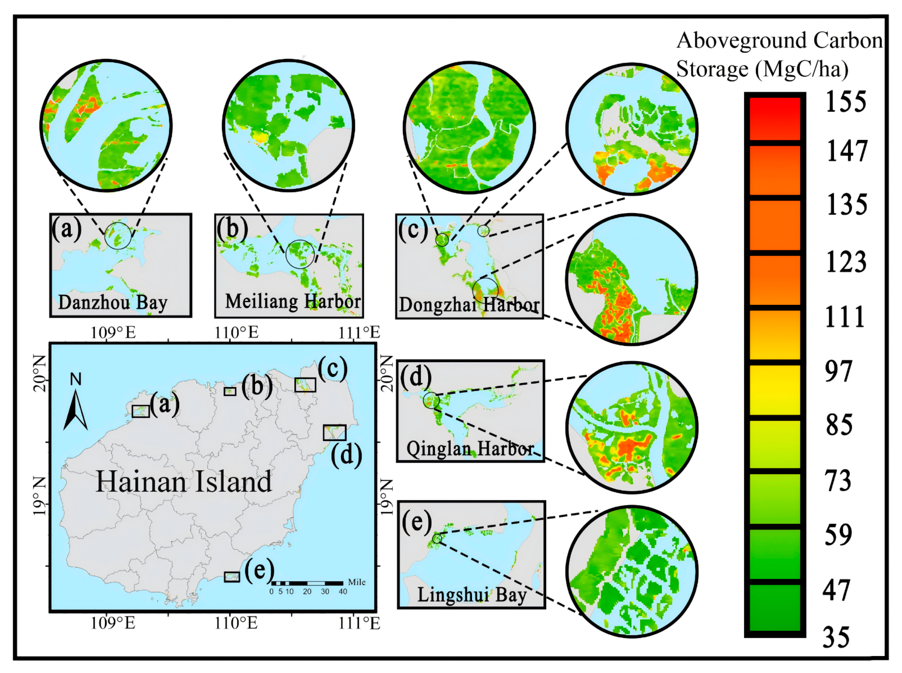
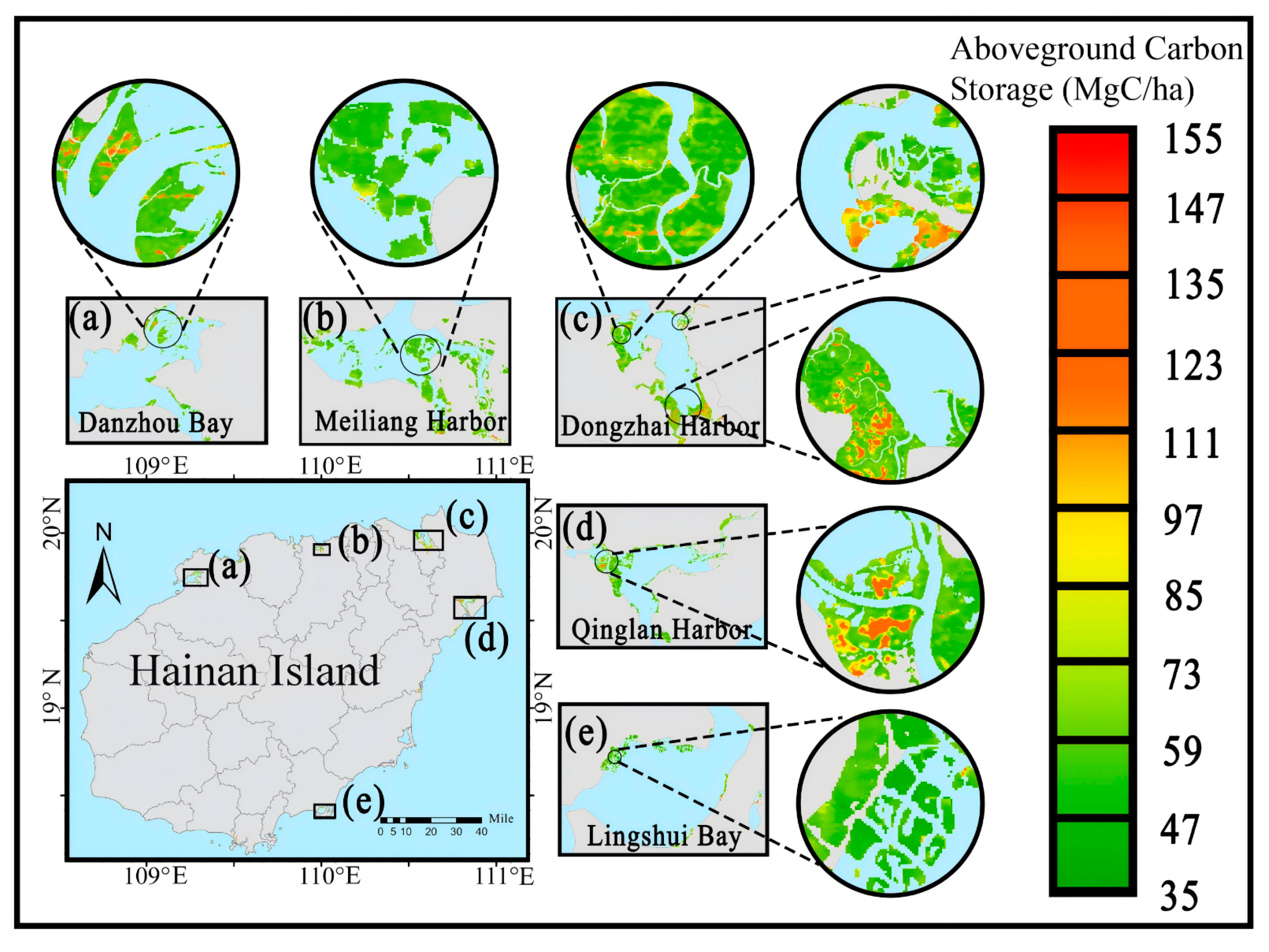
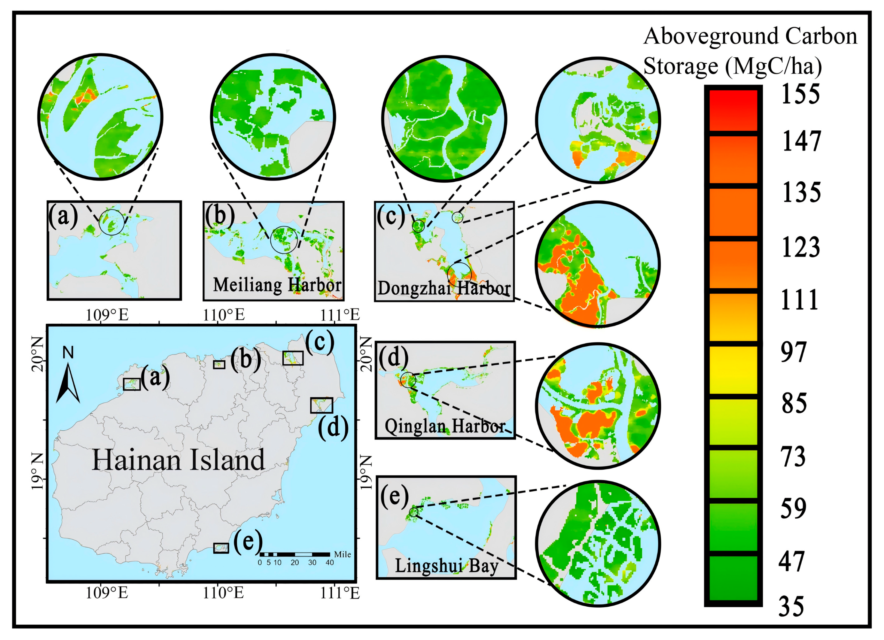
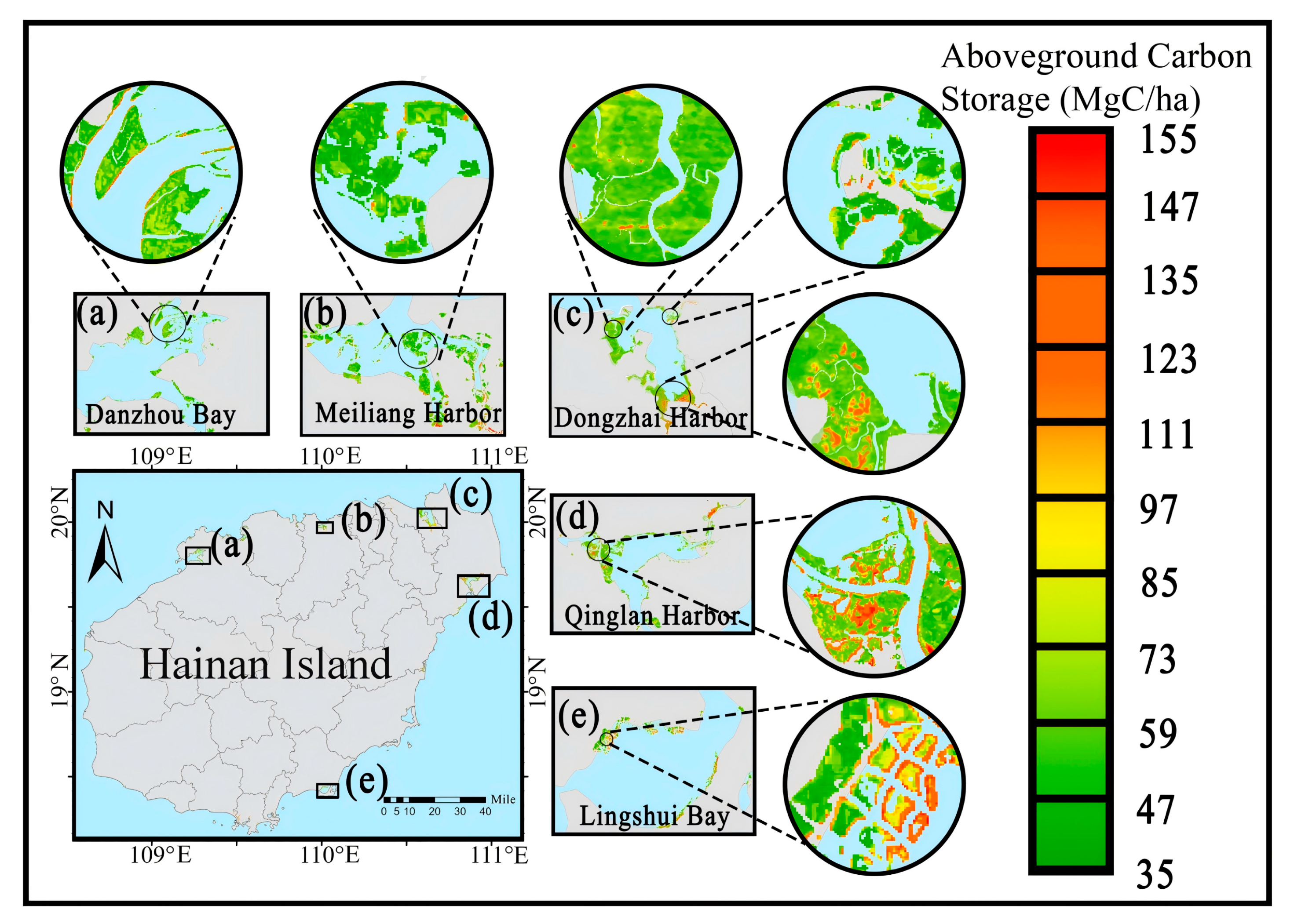
Based on the estimation results from the random forest (RF) model, the aboveground carbon storage (ACS) of Hainan’s mangrove forests exhibited a steady upward tendency between 2019 and 2023. It is acknowledged that mangrove-specific carbon fractions reported for Chinese mangroves typically range from 0.45 to 0.48. Using a uniform factor of 0.5 may lead to a slight overestimation of aboveground carbon storage; however, this systematic bias does not affect the relative spatial patterns or temporal trends emphasized in this study. Spatial distribution analysis indicated that high-carbon storage areas were concentrated in the eastern and northern coastal zones, particularly around Dongzhai Harbor, Qinglan Harbor in Wenchang, Qionghai, and the coastal regions of Haikou. These areas feature extensive mangrove coverage, mature stands, and well-established community structures, demonstrating a robust carbon sequestration capacity. In contrast, the mangrove areas in the western and southern regions (such as Dongfang, Ledong, and Sanya) were relatively small and scattered, with generally low aboveground carbon storage. This reflects regional variations in the progress of mangrove restoration and ecological productivity (Figure 13, Figure 14, Figure 15, Figure 16 and Figure 17).
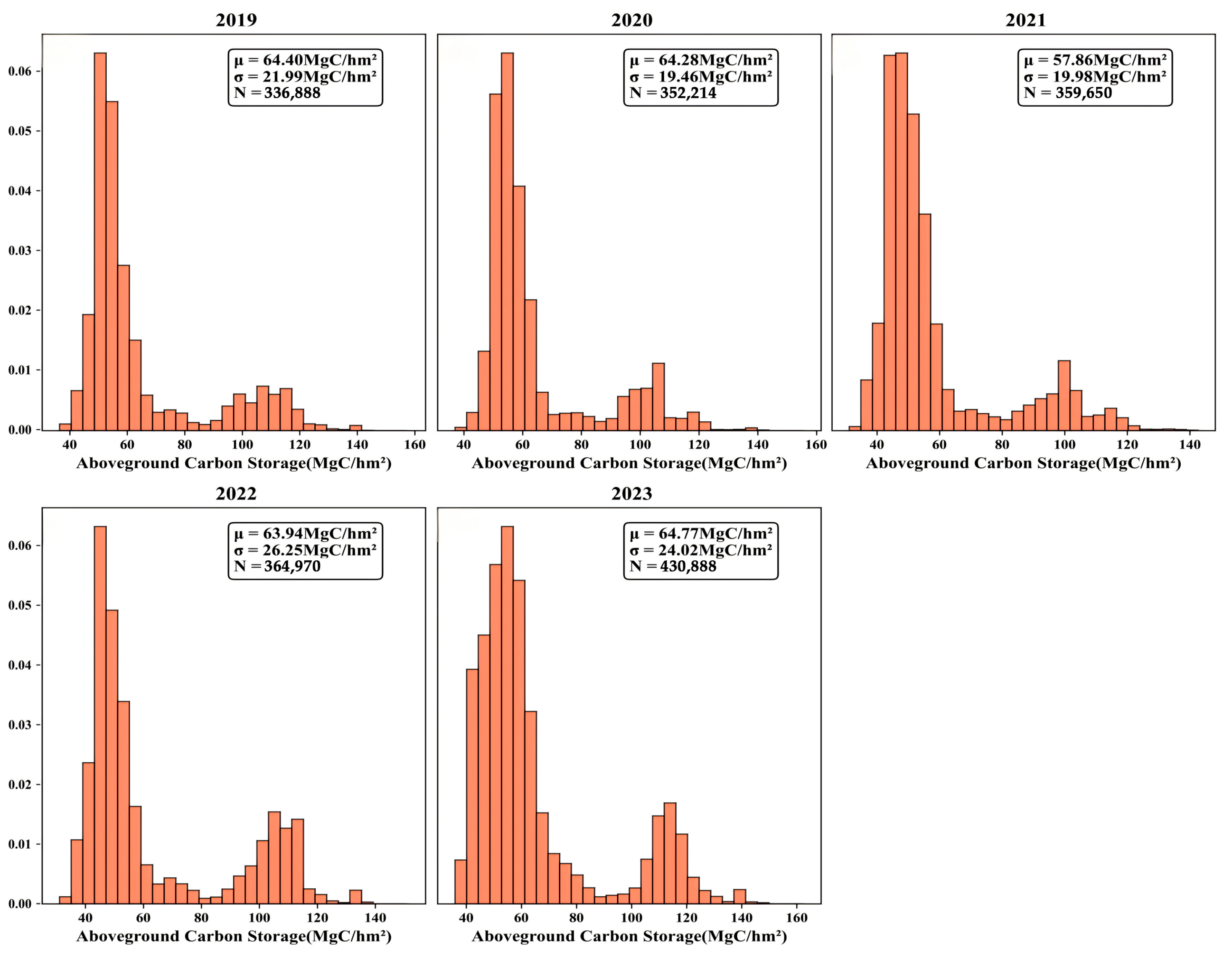
From an interannual perspective, the aboveground carbon storage of Hainan’s mangrove forests exhibited an overall dynamic pattern of initial decline, followed by an increase between 2019 and 2023. From 2019 to 2020, the island’s total carbon storage remained relatively stable before declining in 2021. In the absence of independent disturbance records, this reduction is more appropriately interpreted as a short-term fluctuation associated with increased spatial heterogeneity and asynchronous growth processes across different mangrove regions, rather than a confirmed ecosystem-wide carbon loss. Subsequently, Carbon storage increased again in both 2022 and 2023, suggesting that the Hainan mangrove ecosystem is resilient to short-term fluctuations. Total aboveground carbon storage increased from 254.30 GgC in 2019 to 278.79 GgC in 2023, corresponding to an average annual growth rate of approximately 4.8%. This demonstrates the continuous enhancement of the carbon sink function within mangrove ecosystems (Figure 18). The distribution of aboveground carbon storage (Figure 18) shows a clear bimodal pattern, suggesting the coexistence of mangrove stands with different structural characteristics and biomass levels. This pattern likely reflects contrasts between relatively young or regenerating mangroves and more mature, high-biomass stands across the study area. While the arithmetic mean may mask this internal heterogeneity, the present analysis focuses on regional-scale spatiotemporal trends rather than stand-level differentiation. A more detailed separation of these groups, for example, through cluster-based approaches, could be explored in future studies.
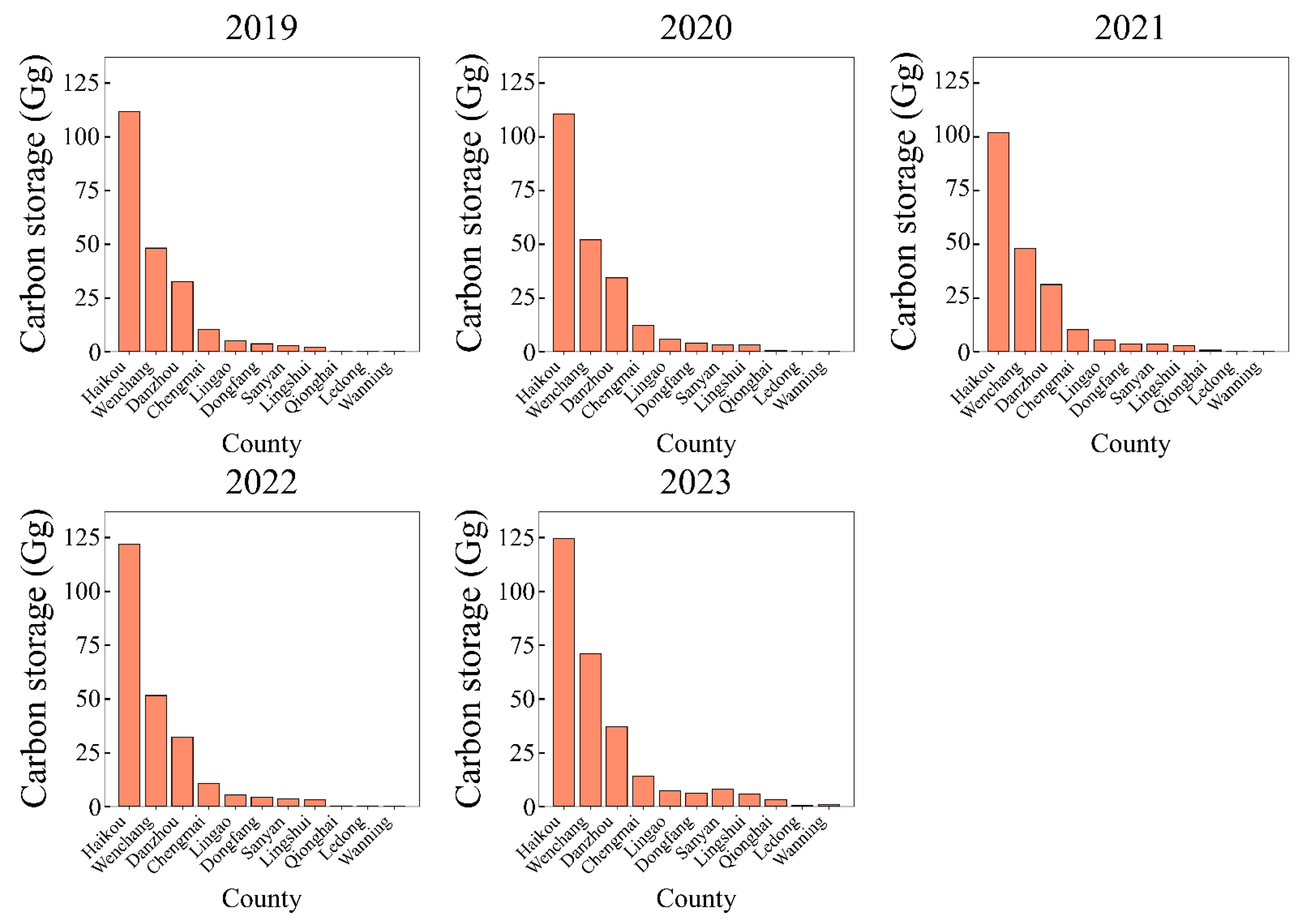
From a spatial perspective, the aboveground carbon storage in the Hainan mangrove forests exhibited marked regional variation across the province. Haikou consistently maintained the highest aboveground carbon storage in the province (110–125 GgC), accounting for over 40% of the island’s total. This was primarily attributable to the extensive mangrove distribution and stable forest structure. Wenchang followed, with carbon storage maintained between 40 and 55 GgC, whereas Danzhou and Chengmai exhibited intermediate levels. In contrast, areas such as Lingshui and Sanya demonstrated lower carbon storage because of mangrove fragmentation and human disturbance (Figure 19).
At the municipal and county level, Hainan’s mangrove aboveground carbon storage increased in 2020, declined in 2021, and gradually recovered between 2022 and 2023. Recovery was particularly pronounced in Wenchang, Danzhou, and Qionghai. Wenchang reached 60.41 GgC in 2023, an increase of 9.04 GgC from 2022, marking the largest recovery. Carbon storage in the Haikou region stabilized after peaking at 101.80 GgC in 2021. In contrast, areas such as Ledong, Dongfang, and Wanning exhibited lower carbon storage with pronounced fluctuations, even recording negative carbon sinks in certain years, indicating slower mangrove recovery in these regions. Overall, the spatial distribution of aboveground carbon storage in Hainan’s mangroves followed a pattern of higher in the north, lower in the south, denser in the east, and sparser in the west. High-carbon storage areas were concentrated in the Beibu Gulf region and eastern coastal zones, whereas the southern and western areas showed slower recovery (Table 9).

4. Discussion

4.1. The Applicability of a Deep Learning-Assisted Multi-Rule Remote Sensing Image Synthesis Method

This study examined the applicability and advantages of different algorithms for mangrove classification, canopy height estimation, and aboveground carbon storage inversion through a comparative analysis of deep-learning-assisted, multi-rule remote sensing image synthesis methods versus multi-source machine-learning models. The results demonstrated that integrating multi-rule image synthesis strategies with deep learning frameworks substantially enhanced mangrove classification accuracy, exhibiting strong robustness and generalization capabilities in complex wetland environments. The NDVI-MAX, MFI-MAX, and EVI-MAX imagery effectively captured the spectral characteristics of mangroves during their active growth phase, reflecting high vegetation density and canopy structural variations. NDWI imagery plays a pivotal role in segmenting mangroves from other water bodies, substantially enhancing the discrimination capability of the classification model. The median synthesis method further mitigated the impact of outliers, enabling the model to achieve an overall classification accuracy exceeding 90%, outperforming existing datasets, such as HGMF_2020, GMW_V3.0_2020, and LREIS_v2_2020 [59]. These results indicate that multi-rule synthetic imagery can effectively enhance the stability and reliability of mangrove identification in tropical wetland environments characterized by frequent cloud cover and complex spectral features.
However, variations persist in the performances of the different spectral indices. NDVI-MAX and EVI-MAX demonstrated outstanding effectiveness in characterizing the peak vegetation growth period. However, they may overemphasize vegetation biomass while overlooking spectral differences between mangroves and water bodies, thereby reducing local classification accuracy. This aligns with prior research findings concerning spectral saturation effects in wetland regions when using single vegetation indices [60]. Therefore, future work should integrate multi-dimensional features, such as tidal variations, topographical factors, and structural parameters, to optimize image synthesis strategies, thereby further enhancing the accuracy and spatiotemporal adaptability of mangrove distribution identification. Overall, the fusion of multi-rule synthesis methods with deep-learning frameworks offers a reliable technical pathway for the refined identification of mangrove ecosystems, demonstrating strong potential for broader applications.

4.2. The Applicability of Machine-Learning-Assisted Multi-Source Remote Sensing Data Fusion Methods

The comparative results of the XGBoost, GBDT, and Random Forest (RF) algorithms in modeling canopy height and aboveground carbon storage indicated distinct performance characteristics across different models when estimating mangrove ecological parameters. The GBDT model demonstrated superior performance in canopy height modeling (R2 = 0.89). It should be noted that, even under low-tide conditions, the extracted ground surface in mangrove environments may still include pneumatophores or prop roots, which can lead to a systematic overestimation of canopy height. Previous studies have shown that canopy height models derived from different remote sensing sources, including airborne LiDAR and other sensor-derived models, can exhibit systematic biases due to differences in sensor characteristics, spatial resolution, and terrain effects, potentially leading to over- or under-estimation of canopy height in mangrove forests. For example, Lagomasino et al. [61] reported measurable discrepancies among multiple canopy height products derived from independent measurements over mangrove ecosystems. In this study, ground point filtering and manual correction were applied to minimize this effect; however, a small residual bias cannot be entirely excluded. Nevertheless, this uncertainty is unlikely to alter the observed spatial patterns or multi-year trends at the regional scale. It should be noted that tidal stage can influence both radar backscatter and optical spectral indices in intertidal mangrove forests, particularly when canopies are partially submerged during high-tide conditions. Although multi-temporal compositing was used to reduce the influence of individual tidal states, explicit tidal height data (e.g., FES2014 or TPXO tidal models) were not incorporated in this study. As a result, residual tidal effects may remain, potentially introducing additional uncertainty in canopy height and carbon estimates at local scales. However, this effect is unlikely to alter the regional spatial patterns and multi-year trends emphasized in this study. It should be noted that the relatively small number of ground reference plots (n = 64) may result in increased uncertainty in model performance metrics, including R2 and RMSE. Furthermore, spatial autocorrelation of residuals was not explicitly quantified (e.g., using Moran’s I), which may partially violate the independence assumption underlying cross-validation. While multi-temporal compositing and spatially distributed sampling were used to mitigate this effect, residual spatial dependence cannot be entirely excluded. Consequently, the reported accuracy metrics should be interpreted as indicative of regional-scale performance rather than precise point-level prediction accuracy. Despite the above-mentioned sources of uncertainty, the comparative analysis of different machine-learning algorithms remains informative for understanding their relative strengths and suitability for modeling mangrove ecological parameters at the regional scale.
Through iterative residual optimization, it effectively captured nonlinear relationships, maintaining a high fitting accuracy even under conditions of limited sample size and low noise levels [60,62]. Concurrently, the enhanced sensitivity of the GBDT to spectral and topographic features improved the interpretability of the model, which is consistent with Pham’s (2020) findings in mangrove biomass inversion [63]. In contrast, XGBoost exhibited high sensitivity to parameter settings and demonstrated poor adaptability when processing low-dimensional data. However, the RF model displayed greater robustness in the carbon storage estimation. Random feature selection and bootstrap resampling reduced the model variance and effectively suppressed overfitting [64]. Moreover, the random forest model exhibited strong robustness to outliers and adapted well to uncertainties in field data, thereby demonstrating favorable generalization performance in carbon storage estimation. However, some studies have indicated that random forests tend to underestimate carbon storage in areas with high biomass [65]. The findings of the present study corroborate this observation. This discrepancy may be attributed to the complex canopy structure of mangrove forests, saturation of remote sensing signals, and uneven distribution of training samples [66,67]. Therefore, in the future, the model structure could be enhanced by integrating ground-based radar data with allometric growth equations, thereby improving the fitting accuracy and ecological interpretability of the model for high-biomass regions.
Overall, the superior performance of the GBDT and RF models in estimating different ecological parameters demonstrates that machine-learning approaches integrated with multi-source data fusion have high feasibility and scientific merit for mangrove ecosystem monitoring. The GBDT is more suitable for handling continuous variables dominated by a single primary factor (such as canopy height), whereas the RF excels in processing multi-dimensional complex feature interactions (such as aboveground carbon storage). These complementary strengths provide methodological guidance for future mangrove ecological parameter retrieval and platform the integrated research that combines multisource remote sensing and ecological modeling.

4.3. Ecological Significance

Based on the inversion results from the GBDT and RF models, this study indicated substantial spatiotemporal variations in the canopy height and aboveground carbon storage of the Hainan mangroves between 2019 and 2023. Overall, Hainan’s mangrove ecosystems tended toward sustained recovery and structural optimization. The average canopy height increased from 4.24 m in 2019 to 4.82 m in 2022 before slightly decreasing to 4.30 m in 2023. Concurrently, aboveground carbon storage (ACS) increased from 254.30 GgC to 278.79 GgC, indicating a sustained enhancement in the ecosystem’s carbon sequestration capacity. This growth pattern demonstrates that Hainan mangroves, driven by recent ecological conservation policies and natural recovery processes, exhibit overall expansion and structural maturation. Changes in mangrove canopy height directly reflect enhanced biomass accumulation and ecological function, consistent with the positive correlation between mangrove height and biomass reported by Hickey et al. [68].
Compared with mangrove forests in other regions, the average canopy height of Hainan’s mangroves is 3.2 m higher than that of northwestern Australia [68], approximately 5.0 m from the Florida mangrove forests in the United States [69], but below the 7.5 m recorded in the African region [21]. The aboveground carbon storage density (63.05 ± 17.33 Mg C ha−1) is higher than that of Australian mangroves (35 Mg C ha−1) but lower than that of Papua, Indonesia (186.36 Mg C ha−1) [70]. This variation reflects the combined influence of climatic conditions, species composition, and human disturbance on the carbon storage capacity. Hainan’s mangroves lie within a tropical monsoon climate zone, where average annual temperatures are 22–26 °C and annual precipitation is 1000–2600 mm, providing favorable growing conditions for mangroves. Concurrently, the region exhibits rich mangrove species diversity, hosting 26 trueand 12 semi-mangrove species. Increased species diversity enhances biomass accumulation and increases carbon storage potential [70].
In terms of spatial distribution, both canopy height and aboveground carbon storage in Hainan’s mangrove forests exhibited pronounced regional variations. The highest carbon storage was found in the Haikou and Wenchang areas, primarily because of the extensive mangrove coverage, older forest age, and high level of protection in these regions. Conversely, the Lingshui and Sanya areas displayed lower carbon storage, largely attributable to the severe fragmentation of mangrove habitats and considerable disturbance from human activities [71]. Moreover, the temporary decline in aboveground carbon storage observed in 2021 may be linked to mangrove damage caused by severe typhoons that year. This phenomenon further demonstrates that extreme weather events can substantially affect both the carbon sequestration capacity and structural stability of mangrove ecosystems. Overall, the spatial heterogeneity of both canopy height and carbon storage reflects the combined effects of environmental factors and human disturbance.
Hainan’s mangrove forest area has seen a net increase of 355.46 ha over the past 5 y, which coincides temporally with the implementation of ecological restoration policies, including the Special Action Plan for Mangrove Conservation and Restoration (2020–2025), suggesting that policy interventions may have contributed to this expansion. It should be noted that this study did not explicitly distinguish between mangrove expansion resulting from artificial planting and that driven by natural recruitment, due to the lack of spatially explicit restoration activity records. Therefore, the relative contributions of different restoration pathways could not be quantitatively separated in this analysis. Since the implementation of the Special Action Plan for Mangrove Conservation and Restoration (2020–2025), restoration projects in mangrove reserves and wetland parks have effectively mitigated ecosystem damage caused by aquaculture expansion and coastal development, thereby providing stable habitat conditions for mangroves. Moreover, the observed increase in mangrove area outside formally protected reserves indicates that additional drivers may also play an important role in mangrove expansion. These drivers may include natural sediment accretion, hydrological changes, and the abandonment or ecological conversion of shrimp ponds and other aquaculture facilities, as reported in previous studies. The combined effects of ecological restoration projects and natural sedimentation processes have gradually led to the spatial consolidation and structural optimization of mangrove forests, enhancing the ecosystem’s self-renewal capacity and carbon sequestration function [62]. These findings indicate that policy interventions and natural succession have produced a substantial synergistic effect on the ecological restoration of the Hainan mangrove forests. In addition, this study focused on mangrove dynamics during 2019–2023 and did not explicitly compare pre-2020 long-term trends (e.g., 2015–2019). Future studies incorporating longer time-series analyses using Landsat or other historical datasets would help to better disentangle policy-driven effects from background expansion trends.
In summary, the spatiotemporal evolution of canopy height and aboveground carbon storage in Hainan’s mangrove forests not only reflects the ecosystem’s recovery process but also validates the effectiveness of ecological restoration policies. The integration of machine learning with multisource remote sensing offers a viable approach for long-term mangrove dynamic monitoring and carbon storage assessment. Future research should combine ground-based observations, radar remote sensing, and ecological modeling to establish a mangrove carbon cycle monitoring system with higher spatiotemporal resolution. This would provide scientific support for mangrove ecological conservation and climate change mitigation at the regional and global scales.

4.4. Study Limitations

Despite the promising performance of the proposed approach, several limitations should be acknowledged. First, the accuracy of canopy height and aboveground carbon storage estimation is constrained by the availability and spatial distribution of ground reference data. The relatively limited number of field plots may introduce uncertainty in model calibration and validation, particularly when extrapolating results to heterogeneous mangrove environments.
Second, technical limitations inherent to Sentinel-2 imagery may affect the retrieval of mangrove structural parameters. The moderate spatial resolution (10–20 m) of Sentinel-2 may not fully capture fine-scale canopy heterogeneity, especially in fragmented or narrow mangrove belts. In addition, optical observations are sensitive to atmospheric conditions and tidal inundation, which may introduce residual uncertainty despite the use of multi-temporal compositing strategies.
Third, the use of NDVI as a key vegetation indicator is subject to well-known limitations. NDVI tends to saturate in high-biomass and dense-canopy conditions, which may reduce its sensitivity to structural variations in mature mangrove forests. Moreover, NDVI can be influenced by background water reflectance and soil moisture, particularly in intertidal environments, potentially affecting its ability to accurately represent vegetation condition. Although additional indices and texture features were incorporated to mitigate these effects, NDVI-related uncertainty cannot be entirely eliminated.
Future research could address these limitations by incorporating higher-resolution optical or radar data, explicitly accounting for tidal dynamics, and integrating alternative vegetation indices or physically based models to improve sensitivity to mangrove canopy structure and biomass.

5. Conclusions

This study systematically enhanced the accuracy of mangrove distribution identification, canopy height inversion, and aboveground carbon storage estimation in Hainan by integrating multi-source remote sensing data, multi-rule image synthesis, and collaborative deep-learning algorithms. Results indicated that the qualityMosaic image synthesis method, which combined the Res34_U-Net with the GEE platform and integrated multiple spectral indices (KNDVI, EVI, NDWI, MFI), significantly improved image quality and classification generalization. This approach achieved an overall mangrove distribution identification accuracy of 92% with a Kappa coefficient of 0.80. Between 2019 and 2023, Hainan’s mangrove area expanded from 3948.83 hm2 to 4304.29 hm2, with an average annual growth rate of 1.8%. Patch connectivity within core protected areas markedly increased, indicating that recent ecological restoration policies had effectively promoted mangrove ecosystem recovery. In the ecological parameter estimation model integrating Sentinel-1/2 and UAV field data, GBDT performed best in canopy height inversion (R2 = 0.89), while RF excelled in aboveground carbon storage estimation (R2 = 0.67). Further calculations revealed an average aboveground carbon storage density of 50.66 Mg C ha−1 for Hainan’s mangroves, with total carbon storage increasing from 254.30 Gg in 2019 to 278.79 Gg in 2023. Significant spatial heterogeneity was observed, with Haikou and Wenchang contributing the most, while Lingshui and Sanya exhibited lower values due to severe fragmentation.
Although this study has made significant progress in mangrove remote sensing monitoring and ecological quantification, there remains room for further improvement. Future efforts could incorporate technologies such as Transformers, 3D-CNNs, and attention mechanisms into deep-learning architectures. Integrating these with multi-source data—including high-resolution LiDAR, hyperspectral imagery, and ground-penetrating radar (GPR)—would strengthen dynamic monitoring and spatial structure analysis capabilities for mangroves. This approach would also enhance the precision of biomass and total carbon storage estimates. Simultaneously, efforts should focus on expanding the regional applicability of the models to scale up findings to larger spatial scales, providing a transferable technical framework for mangrove conservation and ecological management both domestically and internationally. Quantifying mangrove ecosystem services—including carbon sequestration, wind and wave attenuation, and biodiversity maintenance—through ecological models like InVEST would optimize ecological compensation mechanisms and wetland restoration policies. This approach would lay a more robust scientific foundation for sustainable mangrove utilization and enhanced ecosystem resilience.

Author Contributions

Conceptualization, Z.Q.; methodology, Z.L., Z.Y. and Z.Q.; software, Z.L.; validation, Z.L., Z.Y., W.Z., Z.F. and H.P.; formal analysis, Z.L., Z.Y. and Z.Q.; investigation, Z.L.; resources, Z.Q.; data curation, Z.L., Z.Y. and Z.F.; writing—original draft preparation, Z.L. and Z.Y.; writing—review and editing, Z.L. and Z.Q.; visualization, Z.L., Z.Y. and W.Z.; supervision, Z.Q. and P.G.; project administration, Z.Q.; funding acquisition, Z.Q. All authors have read and agreed to the published version of the manuscript.

Funding

This research was funded by “National Natural Science Foundation of China, grant number 32160364”.

Data Availability Statement

Item-Mangrove distribution, canopy height, and above-ground carbon stock data in https://figshare.com/articles/dataset/Mangrove_distribution_canopy_height_and_above-ground_carbon_stock_data_in_Hainan_from_2019_to_2023/29150048?file=54841109 (accessed on 23 December 2025).

Acknowledgments

The authors thank those students who assisted with fieldwork and data collection, and instructors for their constructive comments on the improvement of this study.

Conflicts of Interest

The authors declare no conflicts of interest.

Appendix A

This appendix provides detailed external validation results that complement the internal validation metrics reported in the main text (Table 3). While the main manuscript summarizes key accuracy indicators, such as precision, recall, F1-score, overall accuracy, and kappa coefficient, this appendix presents the complete confusion matrices and class-specific accuracy metrics used to derive these indicators. Specifically, Appendix A Table A1 reports the external validation results of the proposed classification approach in comparison with existing mangrove datasets (HGMF_2020, GMW_V3.0_2020, and LREIS_V2_2020). The table includes producer accuracy, user accuracy, and overall accuracy for mangrove and non-mangrove categories under different compositing rules. These detailed metrics support the conclusions drawn in the main text, including the superior overall precision (90%) and kappa coefficient (80%) achieved by the proposed approach, as well as the high producer accuracy (94.6%) and user accuracy (85.1%) for mangroves under the median compositing rule.
Table A1. Confusion matrix results.
Confusion MatrixReference Data
HGMF_2020MangroveNon-mangroveTotal
Classification ResultsMangrove44256275052
Non-mangrove78345195302
Total5208514610,354
GMW_V3.0_2020
Classification ResultsMangrove31416143755
Non-mangrove206745326599
Total5208514610,354
LREIS__v2_2020
Classification ResultsMangrove39714094380
Non-mangrove123747375974
Total5208514610,354
MR_2020_KNDVI
Classification ResultsMangrove35801663776
Non-mangrove162849506578
Total5208514610,354
MR_2020_MFI
Classification ResultsMangrove32951563451
Non-mangrove191349906903
Total5208514610,354
MR_2020_EVI
Classification ResultsMangrove33081663471
Non-mangrove190349806883
Total5208514610,354
MR__2020_NDWI
Classification ResultsMangrove35151953710
Non-mangrove169349516640
Total5208514610,354
MR__2020_Median
Classification ResultsMangrove44335244687
Non-mangrove77548925667
Total5208514610,354

References

  1. Mumby, P.J.; Edwards, A.J.; Arias-González, J.E.; Lindeman, K.C.; Blackwell, P.G.; Gall, A.; Gorczynska, M.I.; Harborne, A.R.; Pescod, C.L.; Renken, H.; et al. Mangroves enhance the biomass of coral reef fish communities in the Caribbean. Nature 2004, 427, 533–536. [Google Scholar] [CrossRef]
  2. Srikanth, S.; Lum, S.K.Y.; Chen, Z. Mangrove root: Adaptations and ecological importance. Trees 2016, 30, 451–465. [Google Scholar] [CrossRef]
  3. Sarker, S.; Masud-Ul-Alam, M.; Hossain, M.S.; Rahman Chowdhury, S.; Sharifuzzaman, S. A review of bioturbation and sediment organic geochemistry in mangroves. Geol. J. 2021, 56, 2439–2450. [Google Scholar] [CrossRef]
  4. Nagelkerken, I.; Blaber, S.; Bouillon, S.; Green, P.; Haywood, M.; Kirton, L.G.; Meynecke, J.-O.; Pawlik, J.; Penrose, H.; Sasekumar, A.; et al. The habitat function of mangroves for terrestrial and marine fauna: A review. Aquat. Bot. 2008, 89, 155–185. [Google Scholar] [CrossRef]
  5. Donato, D.C.; Kauffman, J.B.; Murdiyarso, D.; Kurnianto, S.; Stidham, M.; Kanninen, M. Mangroves among the most carbon-rich forests in the tropics. Nat. Geosci. 2011, 4, 293–297. [Google Scholar] [CrossRef]
  6. Liao, J.; Zhen, J.; Zhang, L.; Metternicht, G. Understanding dynamics of mangrove forest on protected areas of Hainan Island, China: 30 years of evidence from remote sensing. Sustainability 2019, 11, 5356. [Google Scholar] [CrossRef]
  7. Goldberg, L.; Lagomasino, D.; Thomas, N.; Fatoyinbo, T. Global declines in human-driven mangrove loss. Glob. Change Biol. 2020, 26, 5844–5855. [Google Scholar] [CrossRef]
  8. West, R.C. Mangrove swamps of the Pacific coast of Colombia. Ann. Assoc. Am. Geogr. 1956, 46, 98–121. [Google Scholar] [CrossRef]
  9. Wang, L.; Sousa, W.P.; Gong, P.; Biging, G.S. Comparison of IKONOS and QuickBird images for mapping mangrove species on the Caribbean coast of Panama. Remote Sens. Environ. 2004, 91, 432–440. [Google Scholar] [CrossRef]
  10. Thomas, N.; Lucas, R.; Itoh, T.; Simard, M.; Fatoyinbo, L.; Bunting, P.; Rosenqvist, A. An approach to monitoring mangrove extents through time-series comparison of JERS-1 SAR and ALOS PALSAR data. Wetl. Ecol. Manag. 2015, 23, 3–17. [Google Scholar] [CrossRef]
  11. Spalding, M.; Kainuma, M.; Collins, L. World Atlas of Mangroves; Routledge: London, UK, 2010. [Google Scholar]
  12. Pham, T.D.; Yokoya, N.; Bui, D.T.; Yoshino, K.; Friess, D.A. Remote sensing approaches for monitoring mangrove species, structure, and biomass: Opportunities and challenges. Remote Sens. 2019, 11, 230. [Google Scholar]
  13. Lucas, R.; Otero, V.; Van De Kerchove, R.; Lagomasino, D.; Satyanarayana, B.; Fatoyinbo, T.; Dahdouh-Guebas, F. Monitoring Matang’s Mangroves in Peninsular Malaysia through Earth observations: A globally relevant approach. Land Degrad. Dev. 2021, 32, 354–373. [Google Scholar]
  14. Lorenzo, E.N.; De Jesus, B.R., Jr.; Jara, R.S. Assessment of mangrove forest deterioration in Zamboanga Peninsula, Philippines, using Landsat MSS data. In Proceedings of the Thirteenth International Symposium on Remote Sensing of the Environment; Environmental Research Institute of Michigan (ERIM): Ann Arbor, MI, USA, 1979; pp. 1737–1745. [Google Scholar]
  15. Heumann, B.W. Satellite remote sensing of mangrove forests: Recent advances and future opportunities. Prog. Phys. Geogr. 2011, 35, 87–108. [Google Scholar]
  16. Hamilton, S.E.; Casey, D. Creation of a high spatio-temporal resolution global database of continuous mangrove forest cover for the 21st century (CGMFC-21). Glob. Ecol. Biogeogr. 2016, 25, 729–738. [Google Scholar]
  17. Green, E.P.; Clark, C.; Mumby, P.; Edwards, A.; Ellis, A. Remote sensing techniques for mangrove mapping. Int. J. Remote Sens. 1998, 19, 935–956. [Google Scholar] [CrossRef]
  18. Giri, C.; Ochieng, E.; Tieszen, L.L.; Zhu, Z.; Singh, A.; Loveland, T.; Masek, J.; Duke, N. Status and distribution of mangrove forests of the world using earth observation satellite data. Glob. Ecol. Biogeogr. 2011, 20, 154–159. [Google Scholar]
  19. Zhang, J.; Liu, Z.; Jiang, W.; Liu, Y.; Zhou, X.; Li, X. Application of deep generative networks for SAR/ISAR: A review. Artif. Intell. Rev. 2023, 56, 11905–11983. [Google Scholar] [CrossRef]
  20. Tsokas, A.; Rysz, M.; Pardalos, P.M.; Dipple, K. SAR data applications in earth observation: An overview. Expert Syst. Appl. 2022, 205, 117342. [Google Scholar] [CrossRef]
  21. Simard, M.; Zhang, K.; Rivera-Monroy, V.H.; Ross, M.S.; Ruiz, P.L.; Castañeda-Moya, E.; Twilley, R.R.; Rodriguez, E. Mapping height and biomass of mangrove forests in Everglades National Park with SRTM elevation data. Photogramm. Eng. Remote Sens. 2006, 72, 299–311. [Google Scholar]
  22. Li, J.; Yu, Z.; Yu, L.; Cheng, P.; Chen, J.; Chi, C. A comprehensive survey on SAR ATR in deep-learning era. Remote Sens. 2023, 15, 1454. [Google Scholar] [CrossRef]
  23. Lee, S.-K.; Fatoyinbo, T.E. TanDEM-X Pol-InSAR inversion for mangrove canopy height estimation. IEEE J. Sel. Top. Appl. Earth Obs. Remote Sens. 2015, 8, 3608–3618. [Google Scholar] [CrossRef]
  24. Lagomasino, D.; Fatoyinbo, T.; Castañeda-Moya, E.; Cook, B.D.; Montesano, P.M.; Neigh, C.S.; Corp, L.A.; Ott, L.E.; Chavez, S.; Morton, D.C. Storm surge and ponding explain mangrove dieback in southwest Florida following Hurricane Irma. Nat. Commun. 2021, 12, 4003. [Google Scholar] [CrossRef]
  25. Fatoyinbo, T.E.; Simard, M.; Washington-Allen, R.A.; Shugart, H.H. Landscape-scale extent, height, biomass, and carbon estimation of Mozambique’s mangrove forests with Landsat ETM+ and Shuttle Radar Topography Mission elevation data. J. Geophys. Res. Biogeosci. 2008, 113, G02S06. [Google Scholar] [CrossRef]
  26. Cloude, S.R.; Pottier, E. A review of target decomposition theorems in radar polarimetry. IEEE Trans. Geosci. Remote Sens. 2002, 34, 498–518. [Google Scholar] [CrossRef]
  27. Abdullahi, S.; Kugler, F.; Pretzsch, H. Prediction of stem volume in complex temperate forest stands using TanDEM-X SAR data. Remote Sens. Environ. 2016, 174, 197–211. [Google Scholar] [CrossRef]
  28. Xiao, W.; Cao, H.; Tang, M.; Zhang, Z.; Chen, N. 3D urban object change detection from aerial and terrestrial point clouds: A review. Int. J. Appl. Earth Obs. Geoinf. 2023, 118, 103258. [Google Scholar] [CrossRef]
  29. Ranjan, R.K.; Singh, G.; Routh, J.; Ramanathan, A. Trace metal fractionation in the Pichavaram mangrove–estuarine sediments in southeast India after the tsunami of 2004. Environ. Monit. Assess. 2013, 185, 8197–8213. [Google Scholar] [CrossRef]
  30. Qiu, S.; Ooi, J.L.S.; Chen, W.; Poong, S.-W.; Zhang, H.; He, W.; Su, S.; Luo, H.; Hu, W.; Affendi, Y.A.; et al. Heterogeneity of fish taxonomic and functional diversity evaluated by eDNA and Gillnet along a mangrove–seagrass–coral reef continuum. Animals 2023, 13, 1777. [Google Scholar] [CrossRef]
  31. Jia, X.; Jiang, D.; Tsang, D.C.; Choi, J.; Yip, A.C. Stacking MFI zeolite structures for improved Sonogashira coupling reactions. Microporous Mesoporous Mater. 2019, 276, 147–153. [Google Scholar] [CrossRef]
  32. Jia, M.; Wang, Z.; Mao, D.; Ren, C.; Song, K.; Zhao, C.; Wang, C.; Xiao, X.; Wang, Y. Mapping global distribution of mangrove forests at 10-m resolution. Sci. Bull. 2023, 68, 1306–1316. [Google Scholar] [CrossRef]
  33. Janiesch, C.; Zschech, P.; Heinrich, K. Machine learning and deep learning. Electron. Mark. 2021, 31, 685–695. [Google Scholar] [CrossRef]
  34. Holben, B.N. Characteristics of maximum-value composite images from temporal AVHRR data. Int. J. Remote Sens. 1986, 7, 1417–1434. [Google Scholar] [CrossRef]
  35. Gupta, K.; Mukhopadhyay, A.; Giri, S.; Chanda, A.; Majumdar, S.D.; Samanta, S.; Mitra, D.; Samal, R.N.; Pattnaik, A.K.; Hazra, S. An index for discrimination of mangroves from non-mangroves using LANDSAT 8 OLI imagery. MethodsX 2018, 5, 1129–1139. [Google Scholar] [CrossRef] [PubMed]
  36. Ghosh, S.M.; Behera, M.D.; Paramanik, S. Canopy height estimation using sentinel series images through machine learning models in a mangrove forest. Remote Sens. 2020, 12, 1519. [Google Scholar] [CrossRef]
  37. Chen, Z.; Zhang, M.; Zhang, H.; Liu, Y. Mapping mangrove using a red-edge mangrove index (REMI) based on Sentinel-2 multispectral images. IEEE Trans. Geosci. Remote Sens. 2023, 61, 4409511. [Google Scholar] [CrossRef]
  38. Chen, G.; Azkab, M.H.; Chmura, G.L.; Chen, S.; Sastrosuwondo, P.; Ma, Z.; Dharmawan, I.W.E.; Yin, X.; Chen, B. Mangroves as a major source of soil carbon storage in adjacent seagrass meadows. Sci. Rep. 2017, 7, 42406. [Google Scholar] [CrossRef]
  39. Bunting, P.; Rosenqvist, A.; Lucas, R.M.; Rebelo, L.-M.; Hilarides, L.; Thomas, N.; Hardy, A.; Itoh, T.; Shimada, M.; Finlayson, C.M. The global mangrove watch—A new 2010 global baseline of mangrove extent. Remote Sens. 2018, 10, 1669. [Google Scholar] [CrossRef]
  40. Baloloy, A.B.; Blanco, A.C.; Ana, R.R.C.S.; Nadaoka, K. Development and application of a new mangrove vegetation index (MVI) for rapid and accurate mangrove mapping. ISPRS J. Photogramm. Remote Sens. 2020, 166, 95–117. [Google Scholar] [CrossRef]
  41. Tran, T.V.; Reef, R.; Zhu, X. A review of spectral indices for mangrove remote sensing. Remote Sens. 2022, 14, 4868. [Google Scholar] [CrossRef]
  42. Kuenzer, C.; Bluemel, A.; Gebhardt, S.; Quoc, T.V.; Dech, S. Remote sensing of mangrove ecosystems: A review. Remote Sens. 2011, 3, 878–928. [Google Scholar] [CrossRef]
  43. Zhang, X.; Treitz, P.M.; Chen, D.; Quan, C.; Shi, L.; Li, X. Mapping mangrove forests using multi-tidal remotely-sensed data and a decision-tree-based procedure. Int. J. Appl. Earth Obs. Geoinf. 2017, 62, 201–214. [Google Scholar] [CrossRef]
  44. Shen, L.; Sun, Y.; Yu, Z.; Ding, L.; Tian, X.; Tao, D. On efficient training of large-scale deep learning models. ACM Comput. Surv. 2024, 57, 1–36. [Google Scholar] [CrossRef]
  45. Navarro, A.; Young, M.; Macreadie, P.I.; Nicholson, E.; Ierodiaconou, D. Mangrove and saltmarsh distribution mapping and land cover change assessment for south-eastern Australia from 1991 to 2015. Remote Sens. 2021, 13, 1450. [Google Scholar] [CrossRef]
  46. Baloloy, A.B.; Blanco, A.C.; Candido, C.G.; Argamosa, R.J.L.; Dumalag, J.B.L.C.; Dimapilis, L.L.C.; Paringit, E.C. Estimation of mangrove forest aboveground biomass using multispectral bands, vegetation indices and biophysical variables derived from optical satellite imageries: Rapideye, planetscope and sentinel-2. ISPRS Ann. Photogramm. Remote Sens. Spat. Inf. Sci. 2018, 4, 29–36. [Google Scholar] [CrossRef]
  47. Wicaksono, P.; Danoedoro, P.; Hartono; Nehren, U. Mangrove biomass carbon stock mapping of the Karimunjawa Islands using multispectral remote sensing. Int. J. Remote Sens. 2016, 37, 26–52. [Google Scholar] [CrossRef]
  48. Purnamasari, E.; Kamal, M.; Wicaksono, P. Comparison of vegetation indices for estimating above-ground mangrove carbon stocks using PlanetScope image. Reg. Stud. Mar. Sci. 2021, 44, 101730. [Google Scholar] [CrossRef]
  49. Wicaksono, P. Mangrove above-ground carbon stock mapping of multi-resolution passive remote-sensing systems. Int. J. Remote Sens. 2017, 38, 1551–1578. [Google Scholar] [CrossRef]
  50. Hamdan, O.; Aziz, H.K.; Hasmadi, I.M. L-band ALOS PALSAR for biomass estimation of Matang Mangroves, Malaysia. Remote Sens. Environ. 2014, 155, 69–78. [Google Scholar] [CrossRef]
  51. Lu, Y.; Wang, L. The current status, potential and challenges of remote sensing for large-scale mangrove studies. Int. J. Remote Sens. 2022, 43, 6824–6855. [Google Scholar] [CrossRef]
  52. Xie, Y.; Rui, X.; Zou, Y.; Tang, H.; Ouyang, N. Mangrove monitoring and extraction based on multi-source remote sensing data: A deep learning method based on SAR and optical image fusion. Acta Oceanol. Sin. 2024, 43, 110–121. [Google Scholar] [CrossRef]
  53. Mai, X.; Li, Q.; Xu, W.; Deng, S.; Wang, W.; Wu, W.; Zhang, W.; Wang, Y. Estimation of Mangrove Aboveground Carbon Using Integrated UAV-LiDAR and Satellite Data. Sustainability 2025, 17, 8211. [Google Scholar] [CrossRef]
  54. Komiyama, A.; Ong, J.E.; Poungparn, S. Allometry, biomass, and productivity of mangrove forests: A review. Aquat. Bot. 2008, 89, 128–137. [Google Scholar] [CrossRef]
  55. Kavzoglu, T. Object-oriented random forest for high resolution land cover mapping using quickbird-2 imagery. In Handbook of Neural Computation; Elsevier: Amsterdam, The Netherlands, 2017; pp. 607–619. [Google Scholar]
  56. Chen, T.; Guestrin, C. XGBoost: A Scalable Tree Boosting System. In Proceedings of the KDD ’16: Proceedings of the 22nd ACM SIGKDD International Conference on Knowledge Discovery and Data Mining, San Francisco, CA, USA, 13–17 August 2016. [Google Scholar]
  57. Friedman, J.H. Greedy function approximation: A gradient boosting machine. Ann. Stat. 2001, 29, 1189–1232. [Google Scholar] [CrossRef]
  58. Breiman, L. Random forests. Mach. Learn. 2001, 45, 5–32. [Google Scholar] [CrossRef]
  59. Geng, L.; Che, T.; Ma, M.; Tan, J.; Wang, H. Corn biomass estimation by integrating remote sensing and long-term observation data based on machine learning techniques. Remote Sens. 2021, 13, 2352. [Google Scholar] [CrossRef]
  60. Chen, J.; Li, X.; Wang, K.; Zhang, S.; Li, J.; Sun, M. Assessment of intertidal seaweed biomass based on RGB imagery. PLoS ONE 2022, 17, e0263416. [Google Scholar] [CrossRef] [PubMed]
  61. Lagomasino, D.; Fatoyinbo, T.; Lee, S.; Feliciano, E.; Trettin, C.; Simard, M. A comparison of mangrove canopy height using multiple independent measurements from land, air, and space. Remote Sens. 2016, 8, 327. [Google Scholar] [CrossRef]
  62. Yan, X.; Li, J.; Smith, A.R.; Yang, D.; Ma, T.; Su, Y.; Shao, J. Evaluation of machine learning methods and multi-source remote sensing data combinations to construct forest above-ground biomass models. Int. J. Digit. Earth 2023, 16, 4471–4491. [Google Scholar] [CrossRef]
  63. Pham, T.D.; Le, N.N.; Ha, N.T.; Nguyen, L.V.; Xia, J.; Yokoya, N.; To, T.T.; Trinh, H.X.; Kieu, L.Q.; Takeuchi, W. Estimating mangrove above-ground biomass using extreme gradient boosting decision trees algorithm with fused sentinel-2 and ALOS-2 PALSAR-2 data in can Gio biosphere reserve, Vietnam. Remote Sens. 2020, 12, 777. [Google Scholar] [CrossRef]
  64. Esteban, J.; McRoberts, R.E.; Fernández-Landa, A.; Tomé, J.L.; Nӕsset, E. Estimating forest volume and biomass and their changes using random forests and remotely sensed data. Remote Sens. 2019, 11, 1944. [Google Scholar] [CrossRef]
  65. Roy, M.-H.; Larocque, D. Robustness of random forests for regression. J. Nonparametric Stat. 2012, 24, 993–1006. [Google Scholar] [CrossRef]
  66. Zhu, Y.; Liu, K.; Liu, L.; Myint, S.W.; Wang, S.; Cao, J.; Wu, Z. Estimating and mapping mangrove biomass dynamic change using WorldView-2 images and digital surface models. IEEE J. Sel. Top. Appl. Earth Obs. Remote Sens. 2020, 13, 2123–2134. [Google Scholar] [CrossRef]
  67. Hu, T.; Su, Y.; Xue, B.; Liu, J.; Zhao, X.; Fang, J.; Guo, Q. Mapping global forest aboveground biomass with spaceborne LiDAR, optical imagery, and forest inventory data. Remote Sens. 2016, 8, 565. [Google Scholar] [CrossRef]
  68. Hickey, S.; Callow, N.; Phinn, S.; Lovelock, C.; Duarte, C.M. Spatial complexities in aboveground carbon stocks of a semi-arid mangrove community: A remote sensing height-biomass-carbon approach. Estuar. Coast. Shelf Sci. 2018, 200, 194–201. [Google Scholar] [CrossRef]
  69. Simard, M.; Fatoyinbo, L.; Smetanka, C.; Rivera-Monroy, V.H.; Castañeda-Moya, E.; Thomas, N.; Van der Stocken, T. Mangrove canopy height globally related to precipitation, temperature and cyclone frequency. Nat. Geosci. 2019, 12, 40–45. [Google Scholar] [CrossRef]
  70. Bai, J.; Meng, Y.; Gou, R.; Lyu, J.; Dai, Z.; Diao, X.; Zhang, H.; Luo, Y.; Zhu, X.; Lin, G. Mangrove diversity enhances plant biomass production and carbon storage in Hainan island, China. Funct. Ecol. 2021, 35, 774–786. [Google Scholar] [CrossRef]
  71. Fu, C.; Song, X.; Xie, Y.; Wang, C.; Luo, J.; Fang, Y.; Cao, B.; Qiu, Z. Research on the spatiotemporal evolution of mangrove forests in the Hainan Island from 1991 to 2021 based on SVM and Res-UNet Algorithms. Remote Sens. 2022, 14, 5554. [Google Scholar] [CrossRef]
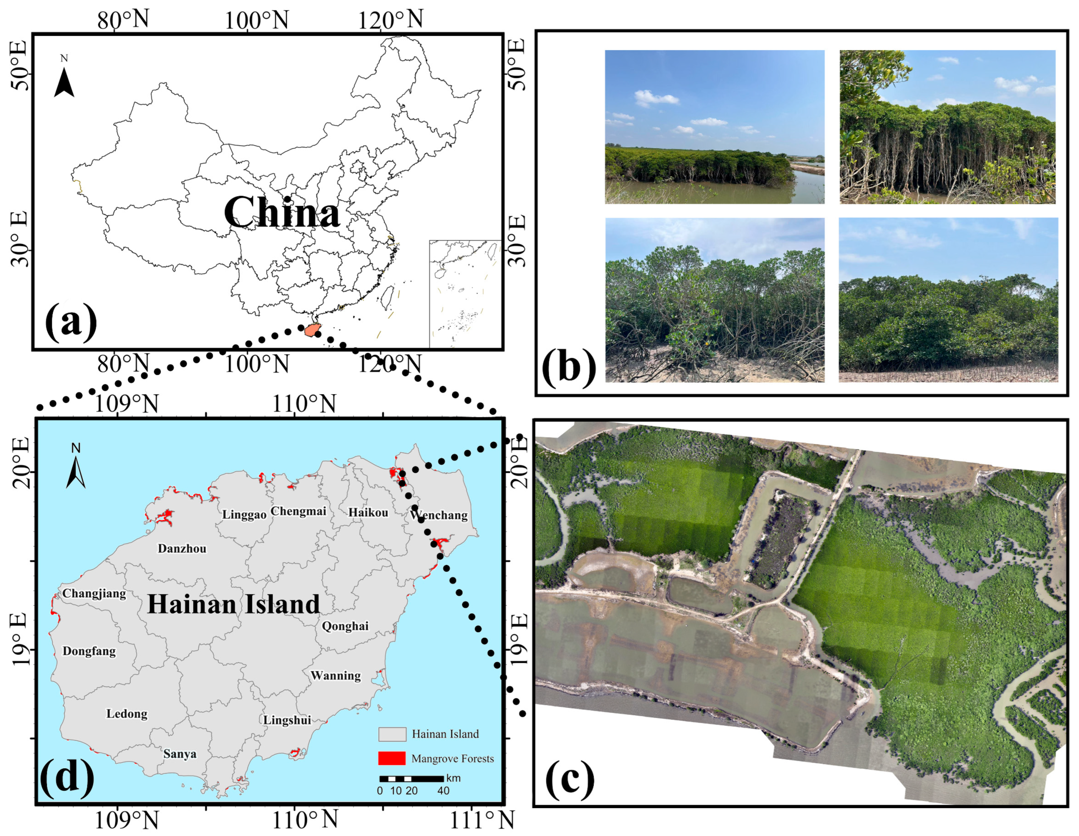
Figure 1. Overview of mangroves in Hainan Island. (a) China; (b) field photo of Dongzhai Harbor mangroves; (c) unmanned aerial vehicle orthophoto of Dongzhai Harbor partial mangrove; (d) mangrove distribution map of Hainan Island.
Forests 17 00131 g001
Figure 2. Network structure of ResNet34. “F(X)” represents the residual term of X, where X is the output feature map of the previous convolutional layer.
Forests 17 00131 g002
Figure 3. The structure of Res34_Unet.
Forests 17 00131 g003
Figure 4. Cross-entropy loss curve of MR_DLM_2020, where the x-axis represents the number of training iterations.
Forests 17 00131 g004
Figure 5. Multi-rule fusion deep learning architecture.
Forests 17 00131 g005
Figure 6. Mangrove distribution range on Hainan Island in 2019–2023.
Forests 17 00131 g006
Figure 7. Canopy height distribution of mangroves in Hainan Island in 2019.
Forests 17 00131 g007
Figure 8. Canopy height distribution of mangroves in Hainan Island in 2020.
Forests 17 00131 g008
Figure 9. Canopy height distribution of mangroves in Hainan Island in 2021.
Forests 17 00131 g009
Figure 10. Canopy height distribution of mangroves in Hainan Island in 2022.
Forests 17 00131 g010
Figure 11. Canopy height distribution of mangroves in Hainan Island in 2023.
Forests 17 00131 g011
Figure 12. Histogram of canopy height distribution from 2019 to 2023.
Forests 17 00131 g012
Figure 13. Distribution of aboveground carbon storage in mangroves of Hainan Island in 2019.
Forests 17 00131 g013
Figure 14. Distribution of aboveground carbon storage in mangroves of Hainan Island in 2020.
Forests 17 00131 g014
Figure 15. Distribution of aboveground carbon storage in mangroves of Hainan Island in 2021.
Forests 17 00131 g015
Figure 16. Distribution of aboveground carbon storage in mangroves of Hainan Island in 2022.
Forests 17 00131 g016
Figure 17. Distribution of aboveground carbon storage in mangroves of Hainan Island in 2023.
Forests 17 00131 g017
Figure 18. Histogram of aboveground carbon storage from 2019 to 2023.
Forests 17 00131 g018
Figure 19. Histogram of aboveground carbon storage by municipality and county from 2019 to 2023.
Forests 17 00131 g019
Table 1. Remote sensing characterization factor.
CategoryRemote Sensing FactorsDescription
Sentinel-2 Band Reflectance 11B2Blue light band, centre wavelength 0.490 μm
B3Green light band, centre wavelength 0.560 μm
B4Red light band, centre wavelength 0.665 μm
B5Vegetation Red Edge Band, Centre Wavelength 0.705 μm
B6Vegetation Red Edge Band, Centre Wavelength 0.740 μm
B7Vegetation Red Edge Band, Centre Wavelength 0.783 μm
B8Near-infrared band, centre wavelength 0.842 μm
B8AVegetation Red Edge Band, Centre Wavelength 0.865 μm
B9Water vapour band, centre wavelength 0.945 μm
B11Shortwave infrared band, centre wavelength 1.610 μm
B12Shortwave infrared band, centre wavelength 2.190 μm
Sentinel-2 Derived Vegetation Index 17RVIRatio Vegetation Index, B8/B4
DVIDifferential Vegetation Index, B8 − B4
WDVIWeighted Difference Vegetation Index, B8 − 0.5 × B4
IPVIInfrared Percentage Vegetation Index, B8/(B8 + B4)
NDVINormalized Vegetation Index, (B8 − B4)/(B8 + B4)
NDI45Optimize the Normalized Difference Vegetation Index, (B5 − B4)/(B5 + B4)
GNDBIGreen Band Normalized Difference Vegetation Index (B7 − B3)/(B7 + B3)
SAVISoil Regulation Vegetation Index, 1.5 × (B8 −B4)/8 × (B8 + B4 + 0.5)
TSAVIConverted soil conditioning vegetation index, 0.5 × (B8 − 0.5 × B4 − 0.5)/(0.5 × B8 + B4 − 0.15)
MSAVICorrected Soil Adjustment Index, (2 − NDVI × WDVI) × (B8 − B4)/8 × (B8 + B4 + 1 − NDVI × WDVI)
ARVIAtmospheric Correction Vegetation Index, [B8 − (2 × B4 − B2)]/[B8 + (2 × B4 − B2)]
PSSRaSimple Ratio Index of Characteristic Pigments, B7/B4
MTCIMedium-resolution terrestrial chlorophyll index, (B6 − B5)/(B5 − B4)
MCARIImproved chlorophyll absorption ratio index, [(B5 − B4) − 0.2 × (B5 − B3)] × (B5 − B4)
S2REPSentinel-2 Red Edge Position Index, 705 + 35 × [(B4 + B7)/2 − B5]/(B6 − B5)
REIPRed-bordered curvature position index, 700 + 40 × [(B4 + B7)/2 − B5]/(B6 − B5)
GEMIGlobal Environmental Monitoring Index, eta × (1 − 0.25 × eta) − (B4 − 0.125)/(1 − B4), In the formula eta = [2 × (B8A − B4) + 1.5 × B8A + 0.5 × B4]/(B8A + B4 + 0.5)
Sentinel-2 Band Texture Features 88
(3 × 3 window)
B1–B12 ContrastContrast reflects the sharpness of an image
B1–12 DissimilarityDiversity is analogous to contrast; the higher the local contrast, the greater the diversity
B1–12 MeanThe uniformity of dispersion of mean-reversed pixel grey values within the image
B1–12 HomogeneityCoherence reflects the uniformity of local grey levels within an image
B1–12 Second MomentThe second-order moment reflects the uniformity and thickness characteristics of texture information in the distribution of grey values within an image
B1–12 EntropyEntropy reflects the complexity of texture within an image
B1–12 VarianceVariance inverse image element value and mean deviation
B1–12 CorrelationThe correlation reflects the similarity between elements in the rows and columns of the grey-scale co-occurrence matrix
Sentinel-1 Normalized Backscatter CoefficientVVVV’s backscatter coefficient
VHVH’s backscattering coefficient
Table 2. Formulae for four vegetation indices.
Vegetation IndexAbbreviationFormula
Kernel Normalized Difference KernelKNDVI t a n ( ( ρ n i r ρ r e d ) / ( ρ n i r + ρ r e d ) 2 )
Enhanced Vegetation IndexEVI 2.5 × ρ n i r ρ r e d ρ n i r + 6 ρ r e d 7.5 ρ b l u e 1
Normalized Difference Water IndexNDWI ( ρ g r e e n ρ n i r ) / ( ρ g r e e n + ρ n i r )
Mangrove Forest IndexMFI [ ( ρ 1 ρ λ 1 ) + ( ρ 2 ρ λ 2 ) + ( ρ 3 ρ λ 3 ) + ( ρ 4 ρ λ 4 ) ] 4
ρ τ i = ρ s w i r 2 + ( ρ i ρ s w i r 2 ) × ( 2190 τ i ) / ( 2190 665 )
Table 3. Internal evaluation results of MR_DLM_2020.
MangroveNon-Mangrove
precision0.920.98
recall0.890.99
F1-score0.910.99
Table 4. External evaluation results of MR_DLM_2020 and other mangrove data.
Data SourceCategoryAccuracy
Producer
Accuracy %
User
Accuracy %
Overall
Precision %
Kappa Coefficient %
HGMF_2020Mangrove87.684.986.372.6
Non-mangrove85.288.0
GMW_V3.0_2020Mangrove83.660.374.150.0
Non-mangrove68.688.0
LREIS__v2_2020Mangrove90.676.384.168.2
Non-mangrove79.392.0
MR_2020_KNDVIMangrove94.868.782.364.7
Non-mangrove75.296.1
MR_2020_MFIMangrove94.868.780.060.1
Non-mangrove75.696.9
MR_2020_EVIMangrove95.263.480.060.2
Non-mangrove72.396.8
MR__2020_NDWIMangrove94.767.581.863.7
Non-mangrove74.596.2
MR__2020_MedianMangrove94.685.190.080.0
Non-mangrove86.395.0
Table 5. Distribution area of mangrove forests in cities and counties from 2019 to 2023.
Municipal and County2019 (ha)2020 (ha)2021 (ha)2022 (ha)2023 (ha)Growth (%)
Chengmai224.66242.14230.47252.44238.92+6.35%
Dongfang75.4880.5584112.6199.38+31.66%
Wenchang947.21977.011009.751021.591083.83+14.42%
Ledong4.194.685.858.528.51+103.10%
Haikou1775.081762.931798.341841.391817.85+2.41%
Sanya78.2784.7490.8100.04107.39+37.20%
Lingshui44.863.967.8973.8694.97+111.99%
Wanning7.78.778.236.5612.31+59.87%
Danzhou644.46655.45653.81671.27668.61+3.75%
Lingao134.12141.97145.39135.55130.76−2.51%
Qionghai12.8627.4320.8810.9641.76+224.73%
Hainan Island3948.834049.574115.414234.794304.29+9.00%
Table 6. Accuracy comparison of three machine-learning models in mangrove canopy height modeling.
Model AlgorithmsR2Bias (m)Relative Bias (%)RMSE (m)RRMSE (%)
XGboost0.720.020.611.3539.86
GBDT0.890.010.421.3939.84
RF0.830.072.001.3539.76
Table 7. Accuracy comparison of three machine learning models in aboveground carbon storage modeling.
Model AlgorithmsR2Bias (MgC/hm2)Relative Bias (%)RMSE (MgC/hm2)RRMSE (%)
XGboost0.740.700.6020.9035.99
GBDT0.770.430.4219.0136.52
RF0.674.464.3817.3334.05
Table 8. Statistics of average canopy height of mangroves in various counties of Hainan from 2019 to 2023.
Municipal and County2019 (m)2020 (m)2021 (m)2022 (m)2023 (m)
Chengmai4.844.875.224.354.23
Dongfang4.705.465.673.634.24
Wenchang4.625.025.264.874.35
Ledong2.953.623.973.882.59
Haikou4.624.574.804.344.13
Sanya5.415.685.875.324.97
Lingshui3.743.823.803.333.26
Wanning5.495.706.225.834.59
Danzhou4.104.064.143.253.88
Lingao4.644.664.683.943.86
Qionghai5.655.806.055.785.18
Hainan Island4.244.644.704.824.30
Table 9. Carbon sequestration statistics of aboveground biomass in mangroves across counties of Hainan from 2019 to 2023.
Municipal and CountyYearArea (hm2)Aboveground Carbon
Storage Density (Mg C ha−1)
Aboveground Carbon Storage (GgC)Carbon Sink (GgC/yr)
Chengmai2019224.6658.813.21/
2020242.1463.0315.262.05
2021230.4752.3312.06−3.20
2022252.4453.7313.561.50
2023238.9258.4313.960.40
Dongfang201975.4863.184.77/
202080.5563.235.090.32
20218458.224.89−0.20
2022112.6158.016.531.64
202399.3862.886.25−0.28
Wenchang2019947.2156.553.52/
2020977.0158.4957.153.63
20211009.7551.3851.88−5.26
20221021.5950.2951.38−0.51
20231083.8355.7460.419.04
Ledong20194.1967.790.28/
20204.6866.50.310.03
20215.8560.330.350.04
20228.5271.320.610.25
20238.5167.450.57−0.03
Haikou20191775.0854.1696.14/
20201762.9355.3997.651.51
20211798.3456.61101.804.16
20221841.3955.71102.580.78
20231817.8556.29102.33−0.26
Sanya201978.2760.354.72/
202084.7463.735.400.68
202190.856.635.14−0.26
2022100.0456.865.690.55
2023107.3960.466.490.80
Lingshui201944.8059.582.67/
202063.959.633.811.14
202167.8951.863.52−0.29
202273.8653.093.920.40
202394.9758.685.571.65
Wanning20197.761.190.47/
20208.7760.690.530.06
20218.2355.650.46−0.07
20226.5657.170.38−0.08
202312.3164.10.790.41
Danzhou2019644.4660.1538.76/
2020655.4561.0139.991.22
2021653.8157.7637.76−2.22
2022671.2757.6338.690.92
2023668.6161.2840.972.29
Lingao2019134.1256.237.54/
2020141.9759.268.410.87
2021145.3959.538.660.24
2022135.5551.596.99−1.66
2023130.7663.948.361.37
Qionghai201912.86610.78/
202027.43621.700.92
202120.8855.161.15−0.55
202210.9659.010.65−0.50
202341.7660.422.521.88
Hainan Island20193948.8364.40254.30/
20204049.5764.28260.306.00
20214115.4157.86238.11−22.18
20224234.7963.94270.7732.65
20234304.2964.77278.798.01
Disclaimer/Publisher’s Note: The statements, opinions and data contained in all publications are solely those of the individual author(s) and contributor(s) and not of MDPI and/or the editor(s). MDPI and/or the editor(s) disclaim responsibility for any injury to people or property resulting from any ideas, methods, instructions or products referred to in the content.