Article

Age-Based Biomass Carbon Estimation and Soil Carbon Assessment in Rubber Plantations Integrating Geospatial Technologies and IPCC Tier 1–2 Guidelines

by
Supet Jirakajohnkool
1,
Sangdao Wongsai
2,3,
Manatsawee Sanpayao
4 and
Noppachai Wongsai
4,*
1
Department of Sustainable Development Technology, Faculty of Science and Technology, Thammasat University, Pathum Thani 12121, Thailand
2
Department of Mathematics and Statistics, Faculty of Science and Technology, Thammasat University, Pathum Thani 12121, Thailand
3
Thammasat University Research Unit in Data Learning, Thammasat University, Pathum Thani 12121, Thailand
4
College of Arts, Media and Technology, Chiang Mai University, Chiang Mai 50200, Thailand
*
Author to whom correspondence should be addressed.
Forests 2025, 16(11), 1652; https://doi.org/10.3390/f16111652 (registering DOI)
Submission received: 15 August 2025 / Revised: 12 October 2025 / Accepted: 28 October 2025 / Published: 30 October 2025

Abstract

This study presents an integrated framework for spatiotemporal mapping of carbon stocks in rubber plantations in Rayong Province, Eastern Thailand—an area undergoing rapid agricultural transformation and rubber expansion. Unlike most existing assessments that rely on Tier 1 IPCC defaults or coarse plantation age classes, our framework combines annual plantation age derived from Landsat time series, age-specific allometric growth models, and Tier 2 soil organic carbon (SOC) accounting. This enables fine-scale, age- and site-sensitive estimation of both tree and soil carbon. Results show that tree biomass dominates the carbon pool, with mean tree carbon stocks of 66.94 ± 13.1% t C ha−1, broadly consistent with national field studies. SOC stocks averaged 45.20 ± 0.043% t C ha−1, but were overwhelmingly inherited from pre-conversion land use (43.7 ± 0.042% t C ha−1). Modeled SOC changes ( Δ SOC ) were modest, with small gains (2.06 t C ha−1) and localized losses (−9.96 t C ha−1), producing a net mean increase of only 1.44 t C ha−1. These values are substantially lower than field-based estimates (5–15 t C ha−1), reflecting structural limitations of the global empirical ΔSOC model and reliance on generalized default parameters. Uncertainties also arise from allometric assumptions, generalized soil factors, and Landsat resolution constraints in smallholder landscapes. Beyond carbon, ecological trade-offs of rubber expansion—including biodiversity loss, soil fertility decline, and hydrological impacts—must be considered. By integrating methodological innovation with explicit acknowledgment of uncertainties, this framework provides a conservative but policy-relevant basis for carbon accounting, subnational GHG reporting, and sustainable land-use planning in tropical agroecosystems.

1. Introduction

Rubber is a globally important commodity, produced in both synthetic and natural forms. Natural rubber is primarily derived from Hevea brasiliensis, a species extensively cultivated across tropical and subtropical regions [1,2,3]. In recent decades, the expansion of rubber plantations has accelerated, particularly in Southeast Asia and West Africa, where forested and agricultural landscapes are increasingly being converted into rubber monocultures. While this expansion contributes to economic development, it has also raised significant environmental concerns, including carbon storage loss, land degradation, biodiversity decline, and disruption of ecosystem functions [3,4].
The transformation of forests and croplands into rubber plantations significantly alters both above-ground biomass (AGB) and soil organic carbon (SOC) stocks, with direct implications for regional carbon dynamics [4,5]. Accurate and spatially explicit estimation of these carbon pools is critical for assessing the role of rubber plantations in climate change mitigation and for informing sustainable land-use planning and policy [6]. Importantly, however, most SOC in rubber plantations is inherited from pre-conversion land uses, while modeled changes during the plantation cycle ( Δ SOC ) are comparatively small and often much lower than field-based estimates. This nuance highlights the need for cautious interpretation of SOC gains, ensuring that results are framed in terms of inherited versus newly sequestered carbon.
Empirical studies on tree carbon stocks in both natural forests and rubber plantations show substantial variability, driven by environmental and silvicultural factors such as stand age, elevation, and management practices. In rubber plantations, carbon sequestration generally increases with age, particularly during the early phases of stand development. Studies applying species-specific allometric equations [7] and long-term field measurements [8] have demonstrated that rubber trees rapidly accumulate biomass carbon in the early years. A recent global review indicates that well-managed rubber plantations can store carbon at levels comparable to other perennial systems, such as agroforestry and secondary forests [9]. Nevertheless, natural tropical forests typically maintain higher overall carbon stocks, underscoring the importance of integrating rubber systems within broader landscape-level carbon assessments.
SOC plays a central role in plantation sustainability by enhancing soil fertility, water retention, and resilience to climate variability [10]. However, its dynamics in rubber systems remain complex, shaped by prior land use, stand age, management intensity, and site-specific soil and climatic conditions [11]. While perennial crops are often assumed to increase SOC relative to annual systems, findings from the Tropics are mixed. Some studies report gradual SOC recovery under mature plantations, whereas others document declines linked to forest-to-plantation conversion, soil disturbance, or reduced litter inputs [4,10,12,13,14]. Guo and Gifford’s (2002) meta-analysis highlighted consistent SOC losses after forest conversion [15], while Liu et al. [16] showed that forest-to-rubber conversion reduced SOC, but intercropping increased it. Regional studies further emphasize the influence of fine-scale biophysical factors such as soil texture, elevation, and microclimate [17,18,19]. Despite these insights, many large-scale assessments still rely on coarse age classes, static land-use maps, or NDVI-based proxies [20]. Although recent advancements in machine learning and remote sensing have significantly improved AGB estimation in rubber plantations [21,22,23], many of these methods still lack the temporal and spatial resolution necessary for fine-scale carbon accounting. Furthermore, SOC remains underrepresented in spatial models, largely due to limitations in data availability and the absence of robust, transferable estimation frameworks.
Recent innovations in remote sensing, particularly in plantation age mapping, present new opportunities to improve carbon assessments. For instance, annual-scale rubber age maps developed by Chen et al. (2018) [24], Somching et al. (2020) [25], and Wongsai et al. (2025) [26], using time-series satellite imagery, have demonstrated the potential for more dynamic and accurate monitoring of plantation development. When combined with species-specific allometric equations, the Intergovernmental Panel on Climate Change (IPCC) Tier 2 carbon accounting methods, and empirical models of SOC change that incorporate plantation age and site-specific soil properties (e.g., Ledo et al., 2020) [11], these tools enable spatially detailed assessments of both tree and soil carbon across heterogeneous landscapes.
At the same time, advances in high-resolution remote sensing—such as Sentinel-2 multispectral imagery (10–20 m resolution) and UAV-based approaches—have substantially improved the capacity to map plantation structure, stand age, and biomass with fine spatial detail (e.g., Phiri et al., 2020 [27]; Li et al., 2022 [28]). These methods are particularly effective for local-scale assessments and for capturing subtle structural differences in heterogeneous landscapes. However, their relatively short temporal coverage (Sentinel-2 since 2015; UAV surveys since the mid-2010s) limits their ability to reconstruct multi-decadal plantation histories. In contrast, the Landsat archive offers a unique 37-year record that enables long-term tracking of plantation establishment and stand age dynamics across broad landscapes. This study leverages that temporal depth to provide insights at a provincial scale, complementing high-resolution approaches by offering the multi-decadal perspective needed for carbon accounting and policy applications.
Beyond their direct carbon sequestration role, rubber plantations also influence ecological processes such as biodiversity conservation and soil fertility maintenance. Conversion of natural ecosystems into monoculture plantations has been associated with biodiversity loss and soil nutrient decline (e.g., Ahrends et al., 2015 [29]; Warren-Thomas et al., 2015 [3]). These ecological changes are closely linked to carbon accounting because reduced soil fertility can limit long-term productivity and carbon accumulation, while biodiversity decline may reduce ecosystem resilience to climate stressors. Positioning carbon stock estimation within this broader ecological context highlights the dual importance of rubber plantations for both climate mitigation and sustainable land management.
This study develops a spatially explicit framework for estimating both tree biomass carbon and soil organic carbon (SOC) in rubber plantations, using plantation age derived from remote sensing as a central input. Existing approaches often lack the resolution and ecological specificity required to capture dynamic carbon changes across continuously transforming landscapes. By integrating annual plantation age maps, species-specific biomass models, and an empirical SOC change model, this study fills a critical methodological gap: the absence of age- and site-sensitive carbon accounting tools at fine spatial scales. Importantly, we emphasize that while tree biomass stocks can be estimated with relatively high precision, modeled SOC change during the plantation cycle ( Δ SOC ) remains small and conservative compared with field-based measurements. Most of the SOC inventory is inherited from pre-conversion land uses, and Δ SOC values should therefore be interpreted as indicative rather than definitive. By explicitly separating inherited stocks from modeled changes, the framework delivers fine-resolution, age-sensitive estimates of both tree and soil carbon, enabling more transparent assessments of carbon dynamics in rubber-dominated landscapes. Beyond rubber systems, the framework is transferable to other perennial agroecosystems, offering a scalable template for tropical land-use carbon accounting with direct applications for climate monitoring, land-use policy, and subnational greenhouse gas reporting.

2. Materials and Methods

2.1. Study Area

Rayong Province, located in eastern Thailand, lies approximately 189 km southeast of Bangkok and covers an area of 3659 km2 along the northeastern coast of the Gulf of Thailand (Figure 1a). It is one of three designated special development zones under Thailand’s Eastern Economic Corridor (EEC) Development Plan and serves as a key industrial hub, home to the Map Ta Phut Industrial Estate—the largest chemical and petrochemical complex in the country.
The province’s topography is primarily composed of rolling terrain, which accounts for 65% of the total area, followed by hilly–mountainous regions (23.16%) and floodplains (11.40%). Urban and industrial areas are mainly concentrated along the coastal plains, whereas agricultural lands dominate the elevated inland zones, particularly within the Rayong and Prasae watershed regions (Figure 1b).
Rayong experiences a tropical savanna climate, which falls within the tropical moist ecological zone according to the IPCC Climate Classification [30] (Chp3, Figure 3A.5.1, p. 3.47), and more specifically, the tropical moist deciduous forest ecological zone [31] (Chp4, Figure 4.1, p. 4.9). Sea breezes help moderate the region’s temperature, maintaining annual averages between 22 °C and 33 °C. The rainy season extends from mid-May to mid-October and is dominated by southwest monsoon winds, creating favorable conditions for the cultivation of fruits, vegetables, and perennial cash crops such as para rubber trees.
The province’s dominant soils are deep silty sands and clayey sands, covering approximately 65.28% of the total land area. According to the Office of Agricultural Economics (OAE, 2023) [32], Rayong ranked first among the seven eastern provinces in terms of rubber cultivation, accounting for 29.9% of the region’s total rubber plantation area. In 2021, the Agricultural Map for Adaptive Management (Agri-Map) system reported that approximately 900.48 km2 of titled land was used for rubber cultivation [33]. In contrast, Land Use and Land Cover (LULC) data from the Land Development Department (LDD, 2024) estimated a higher rubber cultivation area of 1348 km2 (Figure 1b), making rubber the dominant crop in the province—covering 56.9% of all agricultural land—followed by pineapple at 8.8% and cassava at 7.9%.

2.2. Data

2.2.1. Landsat Time Series

This study utilized a time series of Landsat Collection 2 (C2) Tier 1 Level-2 (L2) Surface Reflectance (SR) imagery accessed via the Google Earth Engine (GEE) platform. Landsat was chosen for its 30-m spatial resolution, consistent radiometric quality, and extensive 37-year archive, making it ideal for long-term land-use monitoring. While MODIS offers higher temporal frequency, its coarse resolution (250–500 m) is unsuitable for detecting smallholder rubber plots. Sentinel-2 provides finer spatial detail (10–20 m) but lacks the historical depth, with continuous data available only since 2015.
Although Sentinel-2 (10 m) offers higher spatial resolution, its short temporal coverage limits its suitability for reconstructing multi-decadal plantation histories. To maintain methodological consistency across the 1988–2024 study period, Landsat (30 m) imagery was exclusively employed. This ensured a harmonized analysis of long-term dynamics at the provincial scale, though very smallholder plantations may be underrepresented. Future research could combine Sentinel-2 with land use/land cover (LULC) and land title maps, together with object-based segmentation, to enhance smallholder-focused assessments. Thus, Landsat remains the most appropriate source for efficient time-series analysis across large landscapes and retrospective plantation age mapping in this study. The imagery was acquired from two adjacent scenes—Path 128, Row 51, and Path 129, Row 51—according to the Worldwide Reference System-2 (WRS-2), with approximately eight-day acquisition intervals. All available images spanning a 37-year period (from November 1987 to October 2024) were used to generate a time series of annually composited Bare Soil Index (BSI) images [34], providing a comprehensive temporal dataset for analysis and enabling the annual prediction of rubber plantation establishment years.
Our previous study identified two distinct patterns in interannual BSI profiles [26]. The first, during the initial 10–15 years of the 37-year study period, reflects land-use conversion from annual crops, paddy fields, or shrubland to rubber plantations. The second, around after 2010, indicates either rubber replanting or conversion from fruit and mixed orchards. Therefore, the full Landsat time series were used to train a predictive model to capture interannual BSI patterns, enabling accurate estimation of plantation establishment across the study period and various land-use transitions.

2.2.2. Land Use and Land Cover (LULC) Data

LULC data for 10 years (1991, 2001, 2006, 2008, 2010, 2013, 2015, 2018, 2020, and 2024) were obtained from the Land Development Department (LDD), Ministry of Agriculture and Cooperatives of Thailand. The obtained LULC maps were in shapefile vector format, using the WGS 84/UTM zone 47N Coordinate Reference System (CRS) with a map scale 1:25,000. According to LDD, these datasets were derived through the interpretation of aerial photographs and satellite imagery. Each version was developed based on the previous dataset, resulting in progressive improvements in spatial accuracy over time.
LULC data were classified into five primary land cover classes, each subdivided into three hierarchical levels. For this study, only the level-3 land use code “A302,” representing rubber plantations in the 2024 dataset, was used to delineate rubber cultivation areas. Earlier LULC datasets were also used to assess historical land-use changes and associated management practices linked to the establishment years of current rubber plantations.
The 2024 LULC dataset used in this study (code A302 = rubber plantation) was obtained directly from LDD. According to LDD’s official documentation, the overall thematic accuracy of the 1:25,000-scale LULC products ranges between 87% and 92%, based on stratified random field verification. While local misclassification may occur in mixed or fragmented landscapes, this high overall accuracy ensures that potential errors in the rubber plantation mask have a negligible impact on provincial-scale analyses.

2.2.3. Soil Series

A soil series shapefile of Rayong Province was acquired from the LDD, using the same projection and map scale as the LULC data. The dataset includes detailed attribute information such as soil series name and group (as defined by the LDD), local climate classification, particle size distribution (percent sand, silt, and clay), topsoil and subsoil textures, bulk density, and soil temperature. No new soil samples were collected for this study; all soil organic carbon (SOC) estimates were derived from existing soil-series datasets provided by the Land Development Department (LDD). These data were harmonized with the IPCC 2019 [30] Tier 2 reference values and applied as the baseline for SOC estimation. Soil series data were reclassified into IPCC soil classes and harmonized for SOC estimation (details in Supplementary Materials).

2.2.4. Rubber Farmer Registration Database

Rubber farmer registration records from the Rubber Authority of Thailand (RAOT) were used to identify sample rubber plantations for stand age classification. RAOT, a government agency under the Ministry of Agriculture and Cooperatives, is responsible for the integrated management of Thailand’s rubber production system. The registration dataset includes key attributes such as year of planting, rubber tree species, and plantation location, with geographic coordinates (latitude and longitude) representing the plantation center, as well as sub-district and district information. These records were used to define regions of interest (ROI) and evaluate the accuracy of rubber stand age classification outcomes.

2.2.5. Rubber Tree Inventory Survey Data

Rubber tree growth characteristics from sample plantations in the study area were collected to develop an empirical tree growth model for estimating AGB. The sampling design and field survey were conducted under a research project on carbon fixation capacity and sustainable carbon management in rubber plantations during the tapping period, supported by RAOT.
To ensure representativeness across key ecological and management gradients, a stratified random sampling framework was employed. The sample design accounted for three major sources of variation: stand age, fertilization regime, and rubber variety. Stand age was categorized into eight groups (4, 7, 10, 13, 16, 19, 22, and 25 years), each spanning a three-year interval to capture different stages of plantation development. Fertilization practices were classified into three levels—under-fertilization, normal fertilization, and over-fertilization—based on RAOT recommendations. The two dominant rubber clones in the region, RRIM 600 and RRIT 251, were included to represent varietal differences in growth behavior and carbon accumulation potential.
This stratification resulted in 24 sampling categories. For each category, three plantations were randomly selected from the RAOT registration database, totaling 72 plantations across Rayong Province. These plantations were geographically dispersed to reflect variation in soil conditions, topography, and land-use history.
Within each selected plantation, five rubber trees were measured. Three trees were randomly selected, while the other two were chosen to represent the smallest and largest girths based on visual inspection of circumference at breast height (CBH). In total, 360 individual trees were recorded. CBH was measured at 1.37 m (4.5 feet) above ground using a measuring tape and converted to diameter at breast height (DBH). Tree height was recorded using a Nikon Forestry Pro II laser rangefinder. DBH serves as a key indicator of tree size and age, while tree height provides complementary information for estimating total above-ground biomass. The sample of 72 plantations and 360 trees was stratified by stand age, fertilization regime, and rubber variety. This sample size was consistent with prior regional studies of rubber carbon accounting (e.g., Chiarawipa et al., 2012 [35]; Nattharom et al., 2021 [36]) and was adequate for developing age- and site-sensitive models at the provincial scale. The sampling strategy ensured a robust representation of the spatial, temporal, and management diversity within the study landscape.

2.3. Tree and Soil Carbon Stock Estimation Framework for Rubber Plantations

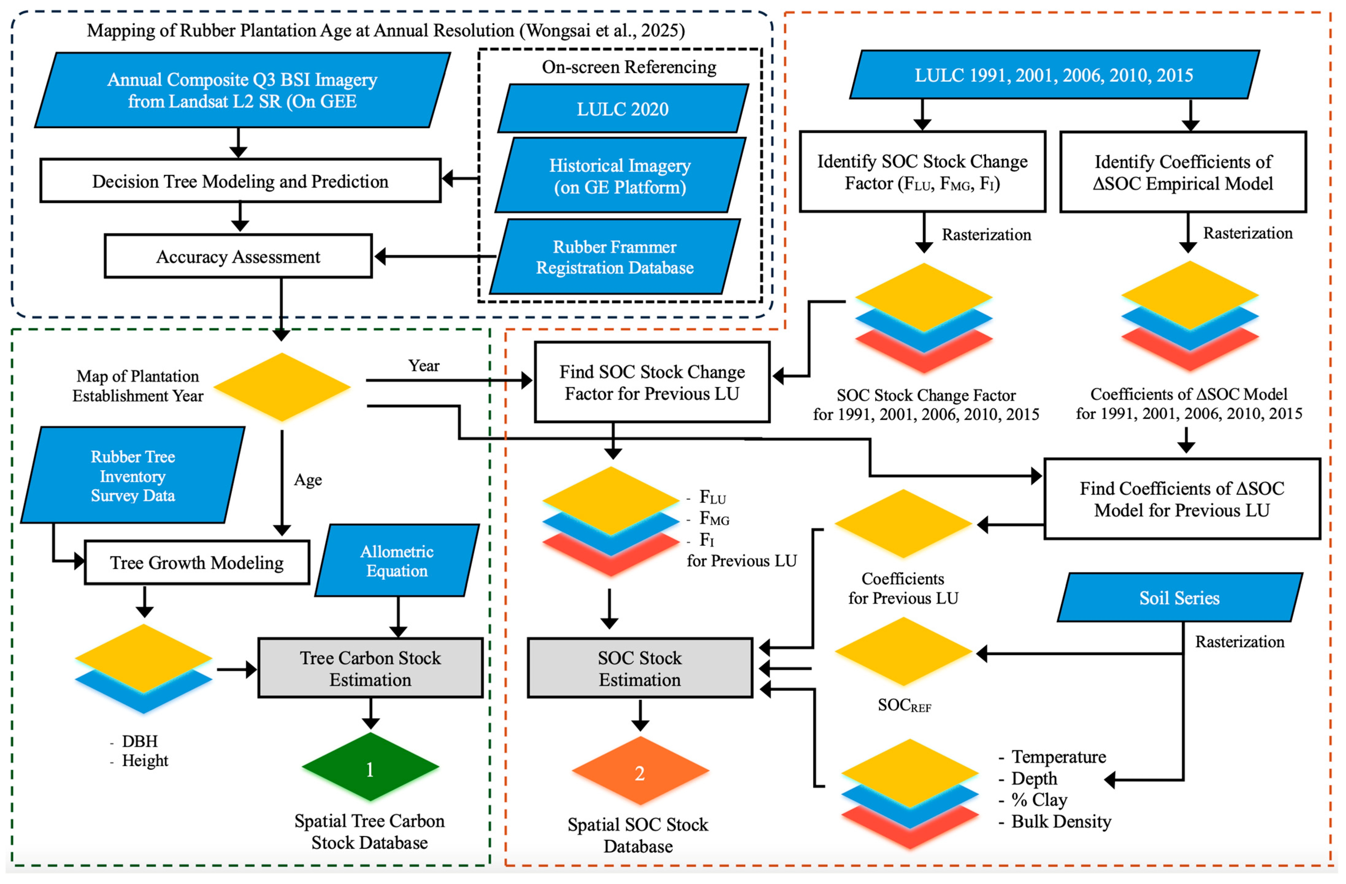
A schematic overview of the framework used to estimate tree and soil carbon stocks in rubber plantations is presented in Figure 2. This framework integrates remote sensing, field inventory data, historical land use, and soil properties to generate spatially explicit carbon stock databases.
The top-left section of the workflow outlines the process for mapping rubber plantation establishment years using annual composite 75th percentile (Q3) BSI imagery derived from Landsat L2 Surface Reflectance (SR) via GEE platform. This mapping process was adopted from our previous study [26]. It involves on-screen referencing using historical imagery, the 2020 LULC dataset, and records from the rubber farmer registration database to create the training dataset, followed by decision tree modeling and prediction of plantation establishment year.
The bottom-left section, newly introduced in this study, focuses on tree carbon stock estimation. Plantation age, derived from the establishment year map, is combined with rubber tree inventory survey data to model tree growth characteristics, specifically DBH and height. These growth parameters are then used to estimate above- and below-ground biomass, resulting in a spatial tree carbon stock database.
The right section of the figure depicts the estimation of SOC stock, which is also newly introduced in this study. This process incorporates IPCC Tier 2 stock change factors—including land use ( F LU ), land management ( F MG ), and fertilizer input ( F I )—along with coefficients from the empirical Δ SOC model. Soil physical properties such as temperature, depth, clay content, and bulk density, derived from soil series data, are also integrated. All input variables are rasterized and processed at the pixel level to estimate SOC dynamics, producing a spatial SOC stock database.

2.4. Data Preparation

2.4.1. Annual BSI Time Series for Predicting Rubber Plantation Establishment Year

Annually composited BSI images were generated from 1895 Landsat SR scenes—including Landsat 5 TM, Landsat 7 ETM+, Landsat 8–9 OLI—using the GEE platform [37]. These composites were used to highlight exposed soil surfaces and support the detection of land-clearing events. For each annual period, images acquired between November of one year and October of the following year were clipped to the study area boundary, cloud-masked using the ‘QA_PIXEL’ quality assurance layer, and processed to compute BSI values. While various formulations of the BSI have been proposed, they generally follow the same structure—comparing visible and shortwave infrared reflectance to the vegetation-sensitive near-infrared reflectance. The standard formulation adopted in this study follows Diek et al. (2017) [34], which is well-suited for Landsat TM, ETM+, and OLI imagery:
BSI   =   SWIR 2   +   Red     NIR   +   Blue SWIR 2   +   Red   +   NIR   +   Blue
Alternatively, some studies substitute SWIR1 with SWIR2, or replace the Blue band with the Green band, and may apply scaling constants to tailor the formulation to specific regions or Landsat sensor platforms [37,38,39,40,41].
BSI values range from –1 to +1 and indicate the degree of land surface exposure. Positive values typically correspond to bare or sparsely vegetated areas—often linked to land clearing activities—while negative values indicate densely vegetated areas. However, anomalously high BSI values can result from persistent cloud cover during the rainy season or from scan line corrector (SLC) errors in Landsat 7 imagery. To mitigate these effects and reduce noise, the Q3 statistic was used during annual compositing [26]. As a result, a 37-year time series of annual Q3 BSI images in the WGS 84/UTM zone 47N CRS was generated and chronologically stacked for further analysis.
To minimize confusion between bare soil and other high-reflectance surfaces such as rooftops, quarries, and sand pits, all annual BSI composites were spatially masked using the 2024 LULC dataset prior to ROI on-screen referencing and model training. Pixels classified as urban, industrial, or barren land in the LULC layer were excluded from the analysis. This masking step effectively reduced false-positive detection of land-clearing events in peri-urban areas.

2.4.2. Soil Organic Carbon Stock Map

Default reference soil organic carbon stocks ( SOC REF ) for mineral soils were assigned to each soil series in the vector soil series map. The attributed fields included topsoil texture descriptions that were matched to six IPCC soil classes as defined in Table 2.3 (p. 2.35) of the IPCC 2019 Guidelines [30] and inferred from the FAO-1990/WRB-2006 soil classification system (see Supplementary Materials for mapping details).

2.4.3. Change in Carbon Stock Before and After Land-Use Conversion

To estimate SOC in mineral soils under rubber plantations, information on the land-use type prior to conversion was required. Level-3 land-use classifications from LULC datasets for nine time points (1991, 2001, 2006, 2008, 2010, 2013, 2015, 2018, and 2020) were reclassified into IPCC land-use management activity categories: land-use system or sub-system ( F LU ), management regime ( F MG ), and organic amendment input ( F I ) [30]. Combined with the year of plantation establishment, this enabled the assignment of default IPCC Tier 2 carbon stock change factors associated with land-use and land management categories at the time of convention supporting SOC change estimation (see Supplementary Materials for full classification).

2.5. Mapping Para Rubber Stand Age

The annual-scale classification of para rubber plantation stand age in this study was adapted from the methodology proposed by Somching et al. (2020) [25] and Wongsai et al. (2025) [26]. The method relies on interannual BSI time series within a seven-year contextual window to detect land-clearing events, which were then used to assign plantation establishment years at the pixel level. The workflow (Figure 2, top-left) includes ROI referencing, supervised model training, and validation. Full methodological details—including feature engineering, sensitivity tests, and validation metrics—are provided in the Supplementary Materials.

2.6. Carbon Stock Estimation

2.6.1. Above- and Below-Ground Biomass

The key predictive variables for estimating AGB in trees are diameter at breast height (DBH) and tree height (H), both of which vary with tree age. To model rubber tree growth in the study area, inventory survey data were used to develop cubic polynomial regression models that capture the non-linear relationships between DBH, H, and tree age. The general form of the regression model is as follows:
y   =   b 0   +   b 1 x   +   b 2 x 2   +   b 3 x 3
A cubic form was selected for its statistical flexibility and strong empirical fit (R2 > 0.95) across the observed age range (5–27 years), offering a practical balance between model simplicity and predictive accuracy without overfitting. Alternative growth functions such as logistic and Chapman–Richards were also tested, but they underestimated early growth and overemphasized long-term decline beyond the commercial rotation age. Given the limited age span of the field data and the ~30-year economic life span of rubber plantations, these more complex sigmoidal models—typically used to capture full biological growth cycles including senescence—were deemed unsuitable [7,42,43]. The cubic polynomial therefore provided the most data-oriented and realistic representation of growth dynamics within the productive phase.
To estimate AGB and below-ground biomass (BGB) of rubber trees, three published allometric models were adopted:
(1)
Witthawatchutikul and Jirasuktaveekul (1988) model [44]
This model was developed from dry weight measurements of rubber trees across 23 plantations of varying ages in the Rayong watershed. Biomass of individual tree components was estimated using the integrated variable DBH 2   ×   H , as follows:
W s   =   0.0556   ×   DBH 2   ×   H 0.866    R 2   =   0.991
W b   = 0.0023   ×   DBH 2   ×   H 1.144    R 2 = 0.878
W l = 0.0705   ×   DBH 2   ×   H 0.572    R 2 = 0.922
  W AGB = W s + W b + W l  
where W s , W b , and W l are the biomass yields (kg) of stem, branches, and leaves, respectively. DBH is measured in centimeters and H in meters.
Although root biomass was not directly measured in this study, below-ground biomass (BGB) was estimated using a root-to-shoot ratio (R), as follows:
W BGB   =   W AGB   ×   R
Root-to-shoot ratios vary widely by species and ecosystem type. In the absence of rubber-specific values, the IPCC 2019 [30] (Chp4, Table 4.4, p. 4.18) recommends the following ratios for tropical moist regions in Asia: (a) R = 0.246 when AGB > 125 t ha−1 and R = 0.323 otherwise. In this study, the threshold was evaluated after converting per-tree AGB to per-area AGB using an assumed planting density of 500 trees ha−1, in line with RAOT recommendations. The Witthawatchutikul and Jirasuktaveekul (1988) model predicted per-area AGB values exceeding 125 t ha−1, which occurred at approximately ≥ 22 years of stand age.
(2)
Chiarawipa et al. (2024) model [45]
This model was developed using five age groups (2, 5, 12, 16, and 26 years) of RRIM 600 rubber trees, each represented by a 1-rai sample plot (approximately 76–80 trees) in Songkhla Province. The allometric equations are as follows:
W s   =   0.1496   ×   DBH 2.2494    R 2   =   0.94
W b   = 0.0023   ×   DBH 2.7559    R 2 = 0.98
W l = 0.0705   ×   DBH 0.8796    R 2 = 0.94
    W BGB = W r = 0.0563   ×   DBH 1.9903    R 2 = 0.9 3
where W r is the root biomass (kg). This model requires only DBH as input, eliminating the need for height measurements.
(3)
Hytönen et al. (2018) model [46]
This model was developed from 18 harvested Hevea brasiliensis (RRIM 600) trees in Songkhla Province. It is widely used in Thailand’s Voluntary Emission Reduction Program (T-VER) projects, supported by the Thailand Greenhouse Gas Management Organization (TGO). The component-wise equations are as follows:
  W l   =   0.001928   ×   DBH 2.499    R 2   =   0.69
W b 1   = 0.007381   ×   DBH 2.551    R 2 = 0.85
W b 2   = 0.01074   ×   DBH 2.382    R 2 = 0.82
  W s = 0.0351   ×   DBH 2.863    R 2 = 0.98
    W BGB = W s ,   r = 0.0 244   ×   DBH 2.470    R 2 = 0.88
where W b 1 and W b 2 are branch biomass for diameters < 3 cm and 3–5 cm, respectively, and W s ,   r represents combined stump and root biomass.
The authors also proposed a simplified model for predicting leafless above-ground biomass (LABG):
  W LABG   =   0.0 5155   ×   DBH 2.783    R 2   =   0.98
Thus, total tree biomass can be estimated by summing all components:
W tree   =   W s ,   r   +   W l   +   W LABG
Similar to the Chiarawipa et al. (2024) model, these equations rely solely on DBH as input and do not require height data.
The three allometric models applied in this study were selected based on their direct applicability to Hevea brasiliensis under Thai growing conditions and their demonstrated use in carbon accounting frameworks. All three were developed from empirical measurements of rubber trees in Thailand, ensuring species specificity and climatic relevance. Using multiple regionally calibrated models allows us to capture a plausible range of biomass estimates for mature and developing plantations, and this inter-model variability is incorporated into our total carbon stock uncertainty estimation.

2.6.2. Estimating Carbon Stock from Rubber Tree Biomass

The carbon stock of an individual rubber tree ( C T , kg C) was estimated as the product of the tree’s total dry biomass ( W T , kg), and the carbon fraction ( CF ) of biomass. In IPCC-aligned REDD+ protocols, carbon in biomass was calculated as [47]:
C T   =   W T   ×   CF  
where W T is the total dry biomass of a rubber tree, computed as the sum of above-ground biomass ( W AGB ) and below-ground biomass ( W BGB ). The carbon fraction ( CF ) represents the proportion of dry biomass composed of carbon. The IPCC default value of 0.47 for tropical tree species, which assumes consistent carbon content across all biomass components (stem, branches, leaves, and roots) in tropical environments was used [31] (Ch4, Table 4.3, p. 4.48). Although field-based allometric models were used to estimate above- and below-ground biomass (aligning with Tier 2-level structural modeling), a Tier 1 carbon conversion factor (CF = 0.47) was applied to convert biomass into carbon stock. This choice reflects the lack of locally measured carbon content values for rubber tree components and follows IPCC guidance for tropical tree species. However, this method aligns with global carbon accounting protocols while also supporting consistency with national reporting practices, as recommended by the TGO. It provides a practical approach for estimating carbon stocks at various scales, from individual trees to entire plantation plots.
At the pixel level, the predicted age of each rubber plantation was used to estimate DBH and height through the tree growth model. These values were then applied in the selected allometric equations to calculate biomass, and subsequently converted into carbon inventory per tree. To estimate total carbon stock per pixel, the carbon content per tree was multiplied by the assumed number of trees per pixel.
A standard planting density of 500 trees per hectare (equivalent to 45 trees per 900 m2 Landsat pixel) was applied, based on the RAOT-recommended spacing of 2.5 × 8 m, which is dominant in flat terrain. This configuration reflects approximately 94% of the rubber cultivation area in Rayong Province, which is classified as flat or gently sloping. Although other alternative spacings are also practiced—such as 3 × 7 m (475 trees ha−1) and 3 × 8 m (419 trees ha−1) in sloped areas (~6% of plantations), or denser arrangements like 2.5 × 7 m (569 trees ha−1) and 3 × 6 m (556 trees ha−1) in newly planted flat zones—the standard density offers a practical and consistent basic for landscape-scale carbon accounting.
While actual stand densities can vary with terrain, clone, and management, and may gradually decline with age, commercial rubber plantations are typically replanted after ~30 years when latex yields diminish. Thus, significant stand-density reductions, such as those observed in natural forests after ~50 years, are rarely encountered in rubber systems. This assumption ensures methodological consistency at the provincial scale, although it may introduce slight over- or underestimation at local scales. Future refinements could incorporate spatially variable densities derived from high-resolution remote sensing or ground survey data.
Finally, the total carbon stock for all rubber plantations in the study area was obtained by summing the carbon stock ( C T ) across all pixels classified as rubber cultivation areas.

2.6.3. Inventory of Soil Organic Carbon (SOC)

Soil carbon inventories encompass estimates of soil SOC stock changes in mineral soils, along with CO2 emissions from organic soils resulting from enhanced microbial decomposition due to drainage and associated land management activities. SOC refers to the carbon stored in the soil in the form of organic matter [48]. Although soils contain both organic and inorganic carbon, land use and management primarily affect organic carbon stocks—particularly in mineral soils. Unlike organic soils, which are rich in organic matter and typically occur in wetlands, mineral soils are moderately to well-drained and dominate most terrestrial ecosystems. Therefore, this study focuses exclusively on mineral soils.
In rubber plantations, SOC is influenced by multiple sources of organic input over the plantation lifecycle, including the decomposition of plant residues, animal manure, organic fertilizer applications, and legacy carbon from previous land uses. While Tier 1 IPCC conversion factors were used for biomass carbon estimation due to the lack of locally measured carbon content data, Tier 2 methods were applied for SOC estimation, taking advantage of available local data such as historical land-use maps, land management factors, and soil physical properties. This mixed-tier approach reflects a balance between methodological rigor and data availability, while remaining consistent with national greenhouse gas inventory guidelines.
In this study, SOC stock at each pixel i within a rubber plantation was defined as the sum of carbon inherited from the previous land use and the net change in SOC during the rubber plantation cycle, as expressed in the following equation:
SOC stock , i   =   SOC prev , i   +   Δ SOC i
In this equation, SOC stock , i   denotes the total SOC stock (in t C/900 m2) at pixel i, the SOC prev , i represents the SOC stock inherited from pre-conversion land use, the Δ SOC i refers to the change in SOC during the plantation period.
The inherited SOC stock, SOC prev , i , estimated using the IPCC default reference value for mineral soils, denoted as SOC REF , and adjusted by relative stock change factors reflecting land use ( F LU ), management practices ( F MG ), and fertilizer input ( F I ). The calculation is based on Equation (2.25) from the IPCC guidelines [30] (Chp2, p. 233), as follows:
SOC prev , i   =   SOC REF , i   ×   F LU , i   ×   F MG , i   ×   F I , i
Here, SOC REF , i is the default IPCC SOC stock value (t C ha−1) under moist/wet tropical climate conditions [30] (Chp2, Table 2.3, p. 2.35), detailed in Table A1. The stock change factors F LU , i , F MG , i , and F I , i are the relative SOC adjustment coefficients for land use, management regime, and fertilizer input, respectively, based on IPCC default values over a 20-year period for cropland. These factors were assigned based on land-use classes from the LULC dataset, using the map year closest to the predicted establishment year of the rubber plantation. Details on the land-use classification and its assignment to each factor level are provided in Table A2. SOC prev , i was multiplied by 0.09 to convert its unit into tonnes of carbon per pixel.
The net change in SOC stock reflects the combined influence of plantation age, previous land use, and site-specific soil characteristics, as highlighted in Ledo et al. (2020) [11]. To enable spatially explicit, pixel-based estimation of SOC dynamics over time, this study adopted the empirical model developed by Ledo et al. for perennial cropping systems. This model was constructed using a Generalized Linear Mixed Model (GLMM) calibrated on a harmonized global dataset of paired SOC observations before and after land conversion [49]. It incorporates both fixed effects (e.g., climate, soil properties, crop age) and random effects representing previous and current land-use types to account for spatial and management variability across regions.
The Δ SOC model of Ledo et al. (2020) was selected because it explicitly incorporates plantation age, land use, management, and input factors, making it suitable for landscape-level assessments in rubber systems. Adoption of this model was also justified by its compatibility with the spatial data structure used in the analysis. A plantation age raster dataset was derived from time-series satellite imagery, and accompanying soil property rasters—such as temperature, clay content, bulk density, and depth—were compiled. These spatial layers collectively provided the necessary covariates for applying the model at the pixel level across the study area, thereby enabling consistent and scalable estimation of SOC change over time.
Following the GLMM model of Ledo et al. (2020), SOC change was estimated as a function of soil, climate, and management predictors. The relative change factor model predicts the log response ratio (lnRR) of SOC after land-use change [50]. The absolute SOC change is then obtained by applying the exponential back-transformation, exp(lnRR) − 1), and multiplying by the inherited SOC stock ( SOC prev ).
Thus, the predicted change in SOC stock ( Δ SOC ) for pixel i is expressed as:
Δ SOC i   =   SOC prev , i   ×   ( e ζ i     1 )  
The term ζ represents the linear predictor, calculated as:
ζ i =   1 100 78.584     0.533   ×   T emp i     0.189   ×   CropAge i     0.018   ×   Depth i     0.056 ×   PerClay i   +   5.352   ×   BD i   +   α PrevLU ( i )   +   γ CurrLU ( i )  
Here, T emp i is the mean annual soil temperature (°C), CropAge i is the perennial crop age (years), and   Depth i is the topsoil sampling depth (cm). The   PerClay i represents the percentage of clay in the topsoil, and BD i is the bulk density of the topsoil in g cm−3. The terms α PrevLU ( i ) and γ CurrLU ( i ) correspond to coefficients of the random effects, capturing the influence of previous and current land-use types, respectively.
In this study, the coefficient for agroforestry systems—including rubber, oil palm, and other perennial woody crops—was applied to represent current land use (CurrLU), as this category aligns well with the characteristics of rubber plantations. The coefficient for previous land use (PrevLU) was assigned based on the estimated year of plantation establishment and a nine-year historical LULC dataset spanning 1991–2020. A series of land-use coefficient maps was generated for each LULC year using values specified in Table A3, covering categories such as annual cropland, fallow land (including abandoned orchards and shrubland), grassland (including abandoned paddy fields and pastures), and natural forest. At the pixel level, the coefficient values were selected from the most recent LULC map prior to the year of plantation establishment.
At the pixel level, the coefficient value for previous land use was selected from the most recent LULC map available prior to the plantation establishment year. This ensured temporal consistency between the legacy land-use effect and the modeling framework proposed by Ledo et al. (2020) [11], thereby maintaining methodological rigor in pixel-based SOC estimation. The resulting Δ SOC values, originally expressed in tonnes of carbon per hectare, were converted to tonnes of carbon per pixel by multiplying by 0.09, corresponding to the 900 m2 spatial resolution of each raster pixel used in this study. Pixels without valid plantation-age information (hereafter referred to as “NA” pixels) were retained in the spatial dataset but excluded from Δ SOC estimation and provincial total calculations. Their potential influence on total SOC was later evaluated through a sensitivity assessment described in the Results section.
The use of these coefficients is supported by several recent studies. For instance, Næss et al. (2023) [51] applied the Ledo et al. (2020) model [11] to assess SOC dynamics in Nordic biofuel cropping systems and confirmed consistent topsoil carbon gains after conversion. A 2023 meta-analysis of perennial systems [50] also cites a model to explain variation in SOC changes, highlighting the importance of predictors such as temperature, clay content, and crop age. Furthermore, Martani et al. (2023) [52] reported approximately a 20% increase in topsoil SOC over 20 years of perennial bioenergy crop cultivation, explicitly referencing Ledo et al.’s methodology. These examples reinforce the empirical robustness and broad applicability of the Δ SOC model across a variety of cropping systems.
Temporal variation in SOC was addressed using a two-part approach. First, the initial SOC stock for each pixel was estimated using IPCC Tier 2 default reference values, adjusted by stock change factors for land use ( F LU ), management ( F MG ), and fertilizer input ( F I ). These factors were assigned based on pre-conversion land-use classifications derived from LULC datasets spanning 1991 to 2020, allowing legacy land-use impacts to be explicitly incorporated. Second, the net change in SOC over time was modeled using the empirical Δ SOC equation from Ledo et al. (2020) [11], which incorporates plantation age, soil characteristics (e.g., clay content, temperature, bulk density, and depth), and random effects associated with prior and current land uses.
All input variables—including soil properties, stock change factors, and land-use history—were processed at the pixel level, enabling the generation of spatially detailed SOC stock maps. This integrated framework captures both the legacy effects of land-use change and the temporal dynamics of SOC under rubber cultivation, providing a scalable and data-driven approach for evaluating carbon changes across heterogeneous tropical landscapes.

2.7. Estimation of Overall 95% Confidence Intervals Using the Delta Method

Uncertainty in the total carbon stock estimate, both tree and soil, arises from multiple sources, including variation in plantation age estimates, the use of different allometric growth models, and such additional steps—converting biomass to carbon and applying planting density and age-class area—also contribute to the final tree carbon stock estimate. On the other hand, different coefficients of variation of adopted IPCC references also contribute to overall SOC stock.

2.7.1. Uncertainty of Tree Carbon Stock

For each plantation age class, the fitted growth models for DBH and height produced a mean biomass per tree and an associated 95% confidence interval (CI). These age-specific CIs were then converted to standard errors (SE = (Upper − Lower)/(2 × 1.96)).
Total carbon stock was calculated as:
C total   =   a = 1 n B ¯ a   ×   CF   ×   PD a   ×   A a
where B ¯ a is the mean biomass per tree for age class a , CF is the carbon fraction (0.47), PD a is the planting density, and A a is the number of pixels representing the mapped area of that age class.
The Delta Method [53,54] was used to propagate variance from age-specific estimates through biomass-to-carbon conversion and spatial aggregation:
Var g X     g μ T g μ
assuming independence between age classes. The overall 95% CI was then:
CI 95 %   =   C total   ± 1.96   ×   Var C total
This approach allows uncertainty from individual plantation-age growth model predictions to be propagated through the biomass-to-carbon conversion and spatial aggregation process, resulting in a single provincial-scale 95% confidence interval that accounts for model-derived variability at the stand level.

2.7.2. Uncertainty of the Inherited SOC Stock from Pre-Conversion Land Use

Uncertainty in SOC prev was quantified using the Delta Method, applied at the pixel level and aggregated to the provincial scale. For each pixel i, inherited SOC was computed as the product of reference SOC ( SOC REF ), and the IPCC Tier 2 change factors for land use ( F LU ), management practices ( F MG ), and fertilizer input ( F I ), as described in Equation (21). Reported uncertainties for each parameter were expressed as coefficients of variation (CVs). The pixel-level relative variance was calculated as the sum of squared CVs:
CV i 2   =   CV SOC REF , i 2 +   CV F LU , i 2 +   CV F MG , i 2 +   CV F I , i 2  
The pixel-level standard error (SE) was derived as:
σ i   =   SOC prev , i   ×   CV i
Aggregate totals were obtained by summing pixel values, while total variance was computed as the sum of squared pixel-level errors (assuming independence):
SOC total   =   i SOC prev , i  
Var total = i σ i 2
SE total = Var total
The provincial-scale mean SOC per hectare was then calculated by dividing the total stock and its standard error by the mapped rubber area. The 95% confidence interval (CI) was reported as the mean ± 1.96 × SE, and also expressed as a relative percentage of the mean.
This hybrid class-level and pixel-wise approach ensures that parameter-level uncertainties ( SOC REF and stock change factors F LU , F MG , F I ) are consistently propagated through to landscape-scale estimates. It allows transparent reporting of both absolute uncertainty (t C ha−1 or total t C) and relative error (%), while clarifying that the uncertainty originates from class-level parameters applied pixel-wise.

2.7.3. Uncertainty of the Changed SOC Stock

Uncertainty in Δ SOC can be assessed using the same Delta Method framework applied to SOC prev . However, Δ SOC is derived from the empirical model of Ledo et al. (2020), which introduces additional sources of uncertainty: (1) uncertainty in predictor variables (e.g., soil temperature, clay content, depth, bulk density), (2) uncertainty in the land-use coefficients ( α PrevLU ( i ) and γ CurrLU ( i ) ) and (3) residual model error, since the Ledo model explains only ~20% of variance.
Because parameter-level uncertainties for the continuous predictors from the soil series dataset were not available, full variance propagation via the Delta Method was not feasible. Instead, Δ SOC was reported as point estimates, with a sensitivity range based on the 95% uncertainty reported for the land-use random effects (previous and current LU). Standard error (SE) for Δ SOC was therefore not provided. This limitation has a negligible impact on provincial-scale confidence intervals, as total uncertainty is dominated by SOC prev , for which uncertainties are fully propagated.
In addition, a simple scenario sensitivity analysis was performed to evaluate the influence of moderate variation in key input parameters on Δ SOC estimates. The analysis tested ± one category shifts in the IPCC Tier 2 stock-change factors ( F LU , F MG , F I ) and ±10% changes in soil bulk density.

3. Results

3.1. Prediction of Rubber Plantation Establishment Year

Analysis of interannual BSI time series revealed two dominant temporal patterns linked to land-use conversion. Type 1 profiles were typically associated with transitions from annual crops, paddy fields, or grasslands to rubber, while Type 2 profiles corresponded to conversions from orchards, degraded forests, or replanting events, as shown in Figure S1.
Recursive Partitioning (RP) models were trained separately for each profile type using a seven-year contextual window. Feature engineering identified a reduced set of predictive variables that maximized computational efficiency without compromising accuracy. Sensitivity analyses of model hyperparameters confirmed stable performance and helped determine optimal complexity parameter values (Figure S1b,c).
Model validation using 1500 independent ROIs demonstrated strong predictive performance, with a Pearson correlation of ρ = 0.977 between actual and predicted plantation years. Approximately 76% of ROIs were correctly classified, and most misclassifications reflected a systematic one-year delay caused by seasonal effects on BSI signals. The regression-based error analysis (RMSE = 1.87 years; adjusted R2 = 0.948) confirmed the robustness of predictions (Figure S2). These metrics confirm the reliability of the predictive model and justify its use for generating a spatial map of rubber plantation age across Rayong Province (Figure 3).
Figures S1 and S2, including examples of BSI profiles, sensitivity tests, feature selection, and validation plots, are provided in the Supplementary Materials.

3.2. Map of Rubber Plantation Age

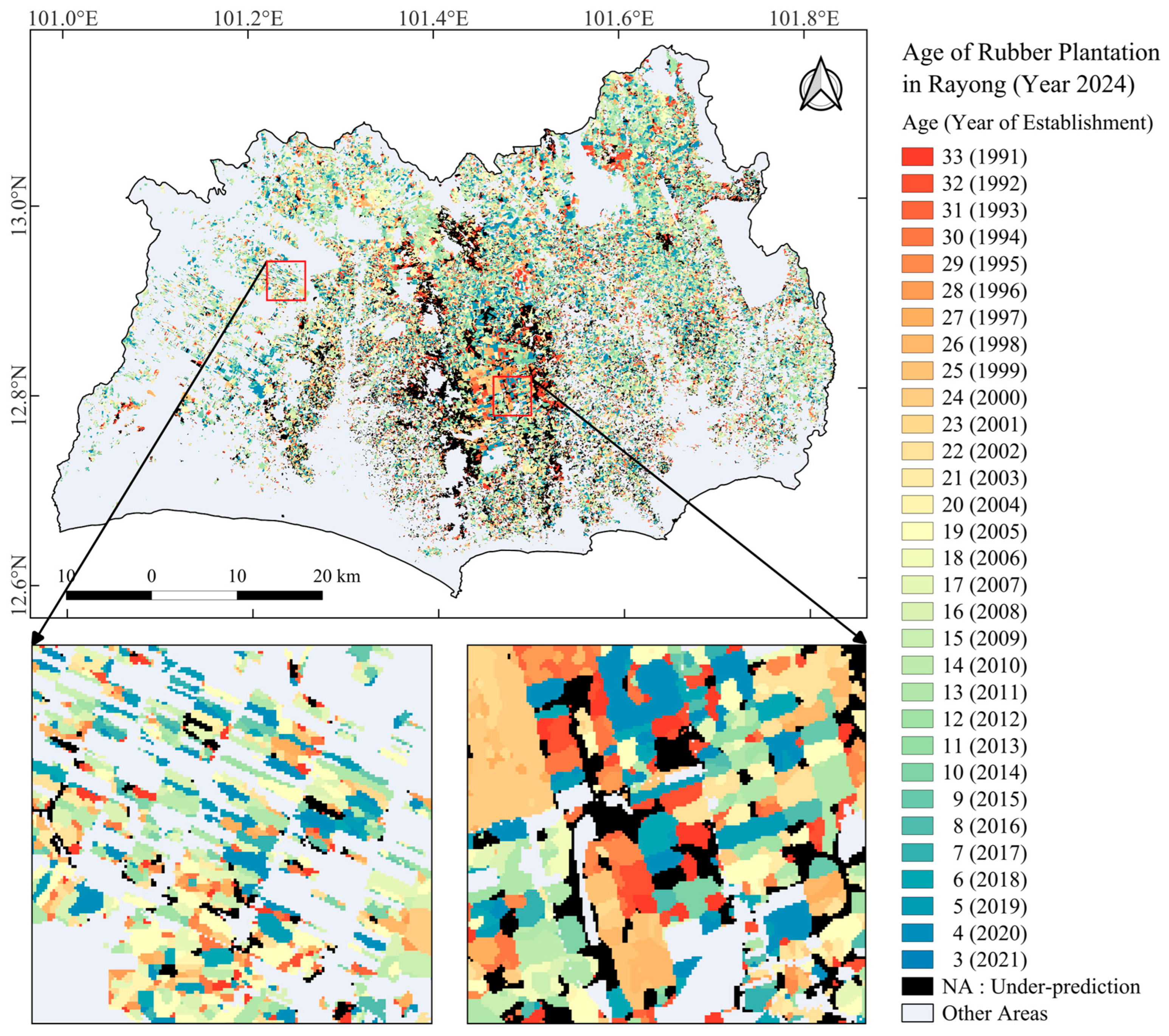
The spatial distribution of rubber plantation ages in Rayong Province was derived by subtracting the predicted plantation establishment year (T0) from the reference year 2024 (Figure 3). The total plantation area in 2024 was approximately 134,938.52 hectares, of which 110,583 hectares were classified with identifiable establishment years using the RP modeling framework.
Plantation age is depicted on the map using a graduated green color scale, where darker shades indicate older stands and lighter shades represent more recent establishments. Areas shown in black correspond to underpredicted zones where the RP model failed to identify an establishment year, totaling about 24,357.15 hectares or approximately 18% of the total plantation area.
Most underpredicted areas are concentrated along the mountainous corridor that runs north–south through the province. This topographic barrier separates the Rayong and Prasae watershed basins, and its complex terrain and vegetation patterns likely reduced model performance due to spectral heterogeneity and persistent cloud cover in the satellite archive.
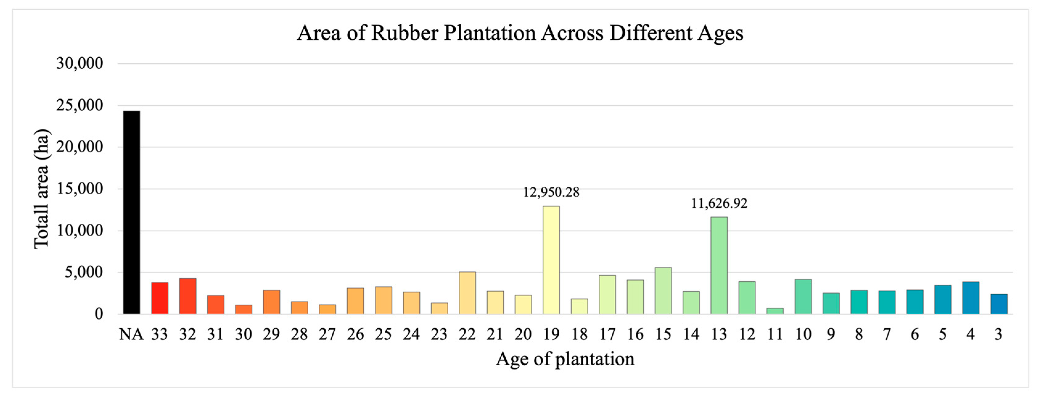
The age distribution of rubber plantations in Rayong Province shows clear peaks at 19 and 13 years (Figure 4), reflecting major planting or replanting waves around 2005 and 2011. Unclassified areas (“NA”), shown in black in Figure 3, represent plantations where establishment year could not be determined. Older stands (31–33 years) persist despite the typical 25–30 year economic lifespan, while younger plantations (3–10 years) indicate ongoing expansion and replanting. Overall, the age structure reflects both legacy cultivation and recent renewal cycles, consistent with long-term management practices in the region.
Figure 3. Map of predicted ages of rubber plantations in Rayong Province, relative to the year 2024. Plantation age is represented using a graduated green color scale, with lighter tones indicating younger stands and darker tones indicating older ones. Areas in black represent plantations where the establishment year could not be determined by the model (underprediction). Insets highlight examples of plantation patch structures at finer spatial scales.
Forests 16 01652 g003
Figure 4. Total area of rubber plantations by age class in Rayong Province, as of the year 2024. Green bars represent the total area (in hectares) for each age group. “NA” indicates areas where plantation age could not be classified.
Forests 16 01652 g004
The accuracy of plantation age prediction was evaluated using 1476 independent validation ROIs. Results showed a strong correlation between observed and predicted establishment years (ρ = 0.98; adj. R2 = 0.95) with an RMSE of 1.87 years. Approximately 76% of plantations were correctly classified, and over 90% were predicted within ±2 years of their true establishment date (Table S2). Most misclassifications involved a one-year overestimation, consistent with seasonal clearance effects reported in previous studies [26]. These results confirm the reliability of the approach for mapping plantation age at the provincial scale, while full accuracy details are provided in the Supplementary Materials (Figure S2).

3.3. Rubber Tree Growth Model

Cubic polynomial regression models with fixed intercepts were developed to characterize the relationship between rubber tree age and two key biometric variables: diameter at breast height (DBH) and tree height (H) (Figure 5). The DBH model was assigned an intercept of 2 cm to reflect the initial diameter of newly planted seedlings, while the height model was set at 1 m, consistent with the average starting height at planting. Further discussion of model assumptions, sensitivity tests, and limitations—particularly regarding fixed intercepts, extrapolation range, and the potential use of mixed-effects formulations—is provided in Section 4.3.3.
A cubic polynomial was selected because it effectively represents the nonlinear growth trajectory of rubber trees, capturing the rapid early increase in DBH and height followed by tapering as stands mature. This model provided a better fit than simpler functions typically used for general tree growth, which extend into senescence but are less applicable to the ~30-year economic life span of rubber plantations.
DBH increased rapidly during the early years of growth before tapering as trees matured (Figure 5a). The model explained 97.4% of DBH variation (R2 = 0.974), demonstrating a strong age-to-diameter relationship. Tree height showed a similar pattern, rising steadily during the first 10–15 years before leveling off (Figure 5b). The height model achieved an even stronger fit, with an R2 of 0.988, indicating highly reliable predictive performance.
The light-blue shaded regions in both panels represent the 95% confidence intervals for the fitted models. These intervals reflect the uncertainty of model estimates across the age range and were calculated based on the standard error of the residuals and the t-distribution corresponding to a 95% confidence level. They provide a statistically grounded range within which the true mean response is expected to lie.
These regression models serve as robust empirical tools for estimating DBH and height from tree age, which are essential input variables for calculating above- and below-ground biomass. The strong model fits confirm the utility of age-based biometric estimation in assessing carbon stock and sequestration potential in rubber plantations.

3.4. Carbon Stock in Rubber Plantations

3.4.1. Tree Carbon Stock

Estimated above-ground biomass (AGB) and below-ground biomass (BGB) of rubber trees aged 3 to 33 years were calculated using three allometric models: Witthawatchutikul and Jirasuktaveekul (1988) [44], Chiarawipa et al. (2024) [45], and Hytönen et al. (2018) [46] (Figure 6). All models showed a consistent increase in biomass with age, reflecting the expected growth trajectory of rubber trees. The Witthawatchutikul and Jirasuktaveekul (1988) model yielded the lowest estimates across all ages, with both AGB and BGB rising steadily until age 22 before BGB declined due to the application of a smaller root-to-shoot ratio once AGB exceeded 125 t ha−1. By contrast, the Chiarawipa et al. (2024) model predicted the highest AGB during the first ~15 years, while the Hytönen et al. (2018) model produced the highest biomass estimates beyond this age.
The average BGB growth rate under the Chiarawipa et al. model was approximately 1.09 kg per year, while the Hytönen et al. model produced a higher BGB increase of 2.36 kg per year. The total biomass predicted by Hytönen et al. (2018) model began to exceed the other two models from age 12 onward. With an average annual increase of approximately 14.21 kg in AGB, the Hytönen et al. model yielded significantly higher biomass estimates in mature plantations. These results highlight the sensitivity of biomass estimates to the selection of allometric models and emphasize the importance of model choice in carbon accounting, particularly for certain age ranges.
Table 1 summarizes predicted biomass statistics for all 360 sampled trees, enabling direct comparison of model outputs against observed field data and quantifying the variation included in the uncertainty analysis. Mean biomass estimates ranged from 220.0 kg under the Witthawatchutikul and Jirasuktaveekul model to 257.0 kg under the Hytönen et al. model, with the Chiarawipa et al. model producing an intermediate value of 242.4 kg. Median biomass was also highest under the Hytönen et al. (2018) model, with Chiarawipa et al. (2014) and Witthawatchutikul and Jirasuktaveekul (1988) models being 3.29% and 9.46% lower, respectively.
The Hytönen et al. (2018) model exhibited the greatest variability (SD = 159.3 kg), reflecting higher predictions in older age classes (Figure 6), while the Witthawatchutikul and Jirasuktaveekul (1988) model showed the narrowest range. These differences highlight the influence of allometric model choice on carbon stock estimates, which was incorporated into the uncertainty analysis. Among the three, the Hytönen et al. (2018) model is considered the most suitable because it was calibrated for Hevea brasiliensis under Thai conditions, is adopted in Thailand’s T-VER carbon accounting framework, and produces estimates consistent with national reporting practices. Notably, it also yields higher average biomass than the other models.
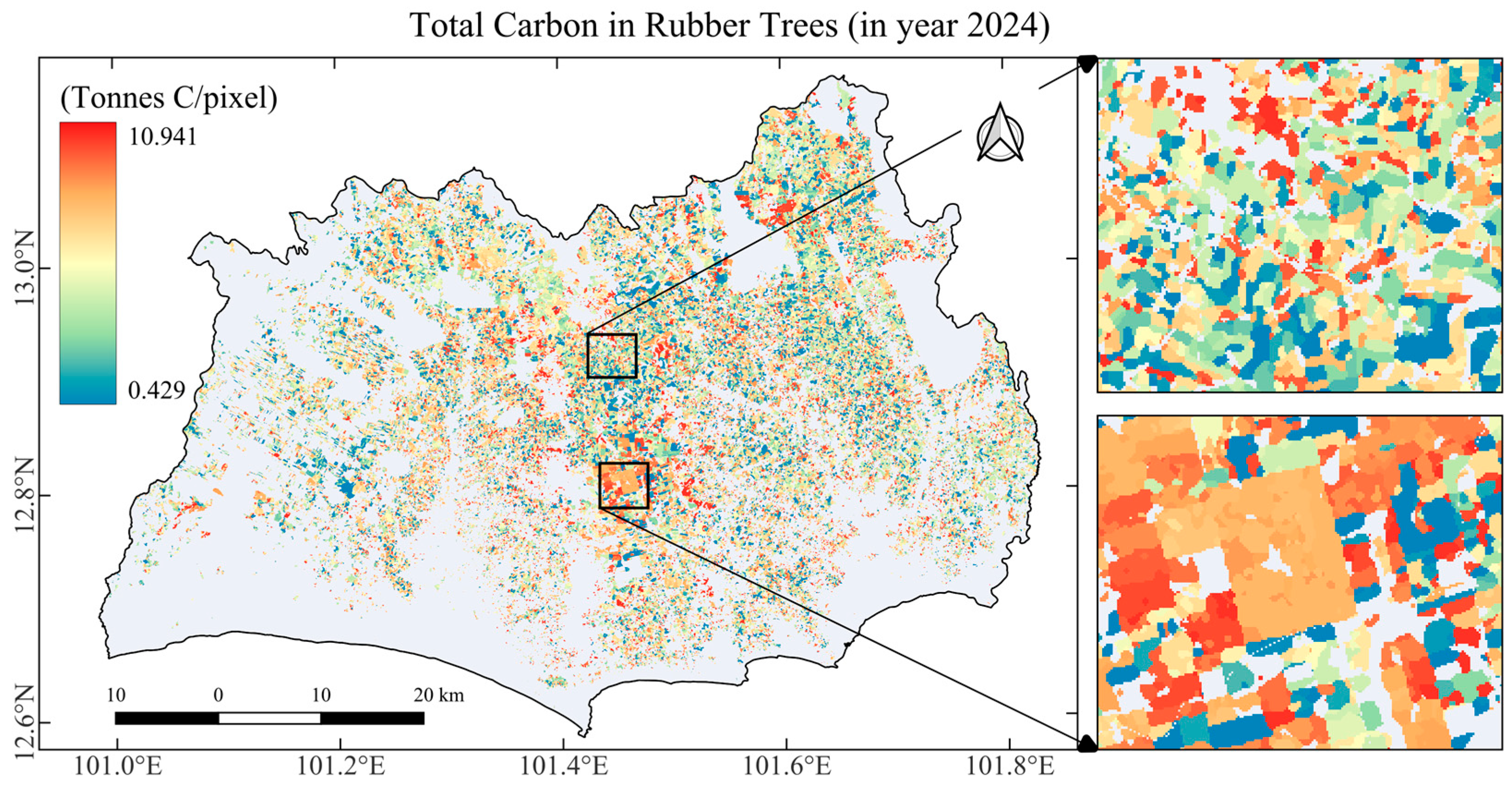
The 2024 spatial distribution of rubber tree carbon stock in Rayong Province, estimated using the Hytönen et al. model, is shown in Figure 7. Carbon stock was calculated by multiplying the carbon content of an individual tree—derived from biomass using a carbon fraction and molecular weight ratio—by the number of trees per 900 m2 pixel (45 trees per pixel based on planting density). Darker green areas indicate higher carbon inventories, corresponding to regions with older plantations, consistent with the age distribution in Figure 3.
The total estimated carbon stocks derived from each model are summarized in Table 2. The Hytönen et al. model produced the highest estimate, at 66.94 t C ha−1, with a 95% confidence interval of 58.19–75.69 t C ha−1. These confidence intervals were obtained using the Delta Method, which accounts for the propagation of uncertainty through nonlinear transformations of DBH and height estimates from regression models. Although the substitution of confidence bounds into nonlinear models does not yield exact confidence intervals, this method provides a valid approximation when the functions are monotonic and the input intervals are sufficiently narrow. It should be noted that total tree carbon estimates were calculated from ~82% of the plantation area where the establishment year could be identified. As ~18% of plantations remain unclassified, the reported totals likely represent a conservative underestimate of the province-wide carbon stock.

3.4.2. Soil Organic Carbon Stock

Analysis of LULC dynamics between 1991 and 2020 shows extensive expansion of rubber plantations, largely replacing annual crops, paddy fields, and mixed orchards. Rubber area grew from 2.6% in 1991 to 45.0% in 2020, with notable increases in the Prasae watershed. In parallel, annual cropland and paddy rice declined steadily, while forest types showed modest reductions. Urban, industrial, and water bodies remained relatively stable, aside from localized reservoir construction. These transitions reflect a province-wide shift toward perennial monoculture systems, providing critical context for evaluating SOC changes.
SOC modeling incorporated spatial layers of soil properties, plantation age, and IPCC Tier 2 stock change factors. Most soils were sandy, with smaller areas of low-activity clay and limited patches of high-activity clay. Biophysical parameters such as soil temperature, depth, clay content, and bulk density showed clear spatial gradients across the province. Plantation age maps highlighted widespread cultivation, with older stands concentrated in central Rayong. Land-use and management factors indicated that most converted areas had previously been cropland or paddy rice, were managed under no-tillage systems, and relied on medium to high synthetic fertilizer inputs. Maps and information of 30-years LULC changes and detailed spatial distributions of soil properties, SOC reference values, plantation age, and IPCC Tier 2 factors, including coefficients used in the empirical Δ SOC model, are provided in Supplementary Materials (Figures S3 and S4).
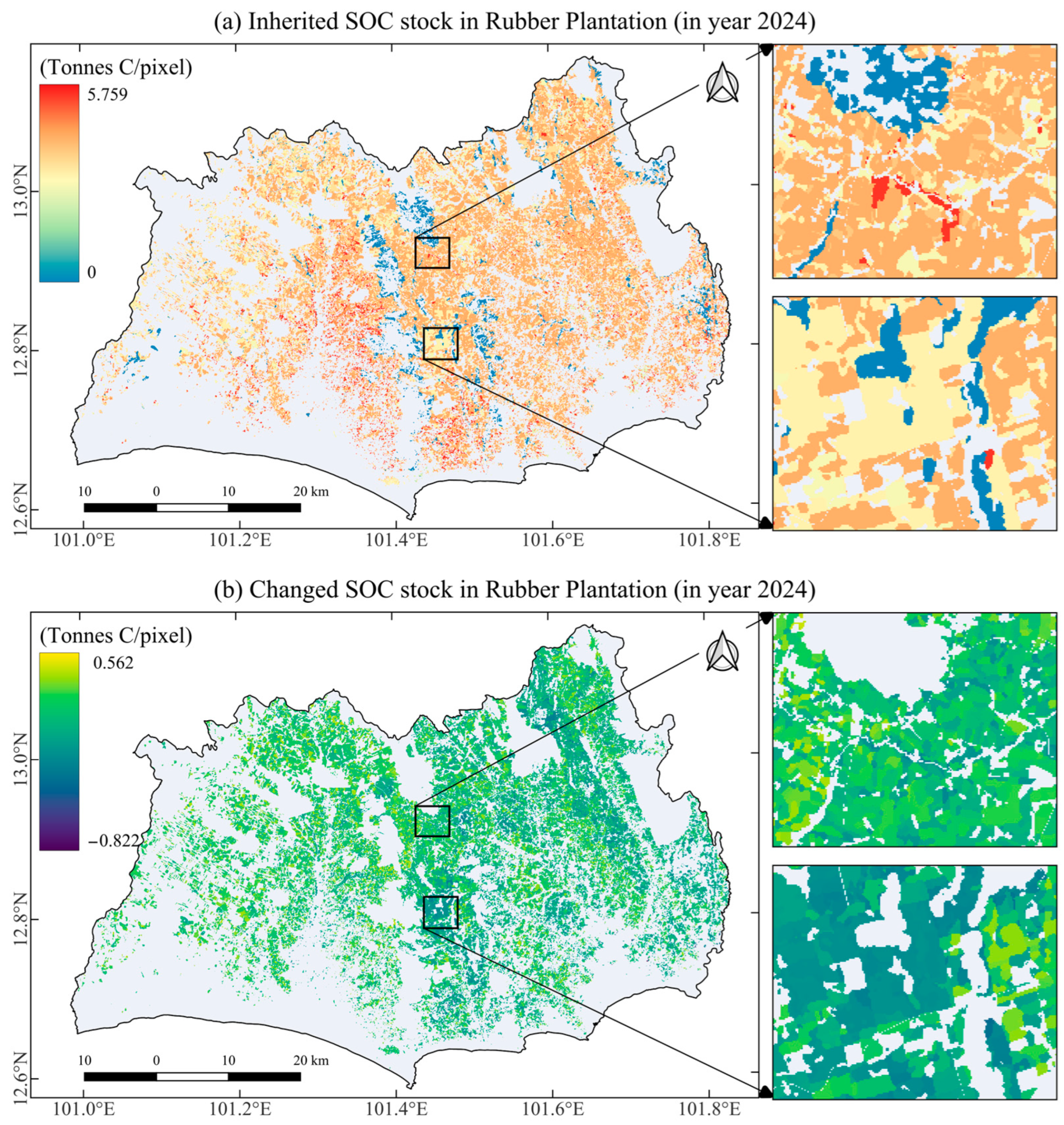
As defined in Equation (20), total SOC stock consists of two components: SOC prev representing inherited carbon stocks from previous land use, and Δ SOC , representing changes during the plantation cycle. The spatial distribution of the estimated SOC inventory in rubber plantations across Rayong Province in 2024 is shown in Figure 8. Inherited SOC range from 1.833 to 5.759 t C/pixel (20.37–63.99 t C ha−1).
The most widespread class, 4.218 t C/pixel (45.412 t C ha−1), accounted for 45.3% of rubber plantation area, primarily associated with low-activity clay (LAC) soils (77.6% of the province) and pre-conversion land uses such as fruit orchards, perennial crop plantations, and rubber replanting sites. Other major classes included 3.150 t C/pixel (35.009 t C ha−1), 2.839 t C/pixel (31.540 t C ha−1), and 5.471 t C/pixel (60.794 t C ha−1), contributing 10.0%, 7.6%, and 4.3% of the plantation area, respectively. Pixels with 0 t C/pixel (blue area in Figure 8a) correspond to rubber plantations located in steep mountainous terrain, slope complex zones, or former paddy fields and floodplains where soil property data were unavailable or soil classes unclassified. These areas represent 5.4% of the total rubber plantation extent in 2024.
Uncertainty in SOC prev was quantified using the Delta Method (see Methods, Section 2.7.2). After propagating parameter-level uncertainties ( SOC REF , F LU , F MG , F I ) to the pixel scale and aggregating across the province, the total SOC prev was 5.60 million t C with a total SE of 1210 t C across plantations with known stand age. When expressed per hectare, this corresponded to a mean of 43.70 t C ha−1 with a 95% CI of 43.68–43.72 t C ha−1 (±0.042%). A per-pixel standard error (SE) map (Figure S5) is provided in the Supplementary Materials.
The relative Δ SOC estimated for the study area ranged from −0.15% to 0.11%. Absolute changes were calculated by multiplying relative Δ SOC   by the baseline SOC stock, then converting to per-pixel units (0.09 ha per pixel) (Figure 8b). Pixel-level values ranged from −0.822 to 0.562 t C/pixel (−9.14 to 6.24 t C ha−1), yielding over 4600 unique values across the province. Most plantations exhibited modest changes with 62.2% of values concentrated between 0 and 3 t C ha−1. Negative Δ SOC occurred in ~21% of plantations, with 13.3% falling between −1 and 0 t C ha−1.
To evaluate age effects, Δ SOC was summarized by plantation stand-age classes using zonal statistics (Figure 9; Table S3). Results showed consistently low values during the first 15 years of plantation growth (mean −1.20 to 0.14 t C ha−1), followed by steady increases with stand age. Gains reached 0.99 t C ha−1 in 16–20-year-old plantations, 1.77 t C ha−1 at 21–25 years, 2.70 t C ha−1 at 26–30 years, and peaked at 3.42 t C ha−1 in stands older than 30 years. Median values mirrored this trend, while pixel-level distributions remained wide (−9.14 to 6.25 t C ha−1) across all age groups.
The boxplots (Figure 9 and Figure S6) show that Δ SOC values increase with stand age, but variability also broadens in older plantations, with wider interquartile ranges and extended whiskers. This indicates that while mean SOC gains rise after ~15 years, site-level responses remain heterogeneous, likely reflecting differences in soil properties and land-use history rather than stabilization of SOC dynamics. Across the province, total SOC gains were 208,405.5 t C (2.06 t C ha−1), offset by losses of −24,915.7 t C (−9.96 t C ha−1), resulting in a net SOC gain of 183,489.8 t C (1.44 t C ha−1) over the study period.
The mean provincial ΔSOC was +1.44 ± 1.87 t C ha−1 based on the 95% uncertainty range from the random-effects terms reported by Ledo et al. (2020) [11]. Because this interval overlaps zero, the modeled ΔSOC should be interpreted as a conservative approximation rather than a statistically significant gain.
To evaluate potential bias from the excluded NA pixels (approximately 18% of the total plantation area), a simple bounding scenario was applied. Assuming that NA pixels have mean SOC values comparable to classified plantations, the total provincial SOC would increase proportionally by ~18%. Under a ±20% variation in that assumption, total SOC varied within ±3% of the reported estimate, indicating minimal bias at the provincial scale.
The observed Δ SOC trajectory reflects both site-level drivers and structural features of the Ledo et al. (2020) model. The model’s negative age parameter dampens early gains, producing stable or slightly increasing values at later stages. Field studies, however, often report initial SOC declines following land conversion due to soil disturbance and reduced productivity, followed by recovery and stabilization [50,55,56]. Meta-analyses further show that SOC in perennial systems generally begins to increase after ~5 years, following a sigmoidal trajectory that slows beyond ~20 years [57]. Local factors, such as soil texture and land-use history, likely explain much of the variation observed among plantations in Rayong.
Although the mean Δ SOC across plantations was 1.44 t C ha−1, this is still below empirical estimates for perennial systems (5–15 t C ha−1). The gap highlights limitations of the Ledo model, particularly its low explanatory power (~20% variance explained). Consequently, SOC totals here are dominated by inherited stocks ( SOC prev ), and modeled Δ SOC should be interpreted as a conservative first-order approximation rather than a direct field-equivalent estimate.
Finally, the total SOC stock—calculated as the sum of inherited SOC and Δ SOC —was estimated at 5.74 million t C (±1257.64 t C SE), corresponding to a mean of 45.20 t C ha−1 (±0.043%). This total was derived from rubber plantation pixels with valid stand-age classification and complete soil-series information, covering around 103,301 ha. This area represents 76.6% of all plantations with known stand age, after excluding approximately 5.4% of those plantations where soil classes were unclassified. Importantly, the uncertainty of this estimate is almost entirely driven by SOC prev , since Δ SOC contributed only ~0.32% of the total stock. Even under a conservative assumption of a coefficient of variation (CV) of 100% for Δ SOC , the relative uncertainty of the provincial total would increase by less than 0.15%. Thus, provincial-scale uncertainty is dominated by SOC prev , for which pixel-level SEs were fully propagated.

4. Discussion

4.1. Comparison with IPCC Default Values and Field Studies

4.1.1. Tree Carbon Stock

This framework provides spatially and temporally refined estimates that differ substantially from generalized IPCC Tier 1 defaults. The IPCC reports an average aboveground biomass (AGB) carbon accumulation rate of 3.0 ± 13% t C ha−1 yr−1 over a 27-year rotation [30] (Chp5, Table 5.3, p. 5.12), with a maximum AGB carbon stock of 80.2 ± 15% t C ha−1 and a mean of 40.1 ± 15% t C ha−1 [58]. These values mask regional variation in stand age, site conditions, and management.
Using the Hytönen et al. (2018) model, our aboveground biomass carbon estimates indicate a sequestration rate of 3.12 ± 10.7% t C ha−1 yr−1 at year 27, which is lower than the annual biomass carbon sequestration reported for PB260 rubber trees in North Sumatra, Indonesia (4.2 t C ha−1 yr−1) [8]. A maximum AGB carbon of 84.34 ± 11.3% t C ha−1, and a mean of 49.25 ± 7.2% t C ha−1 across a 25-year rotation. After convert the whole tree dry biomass to carbon, the mean tree carbon stock was 66.94 t C ha−1 (±13.1%), closely aligned with national field studies: slightly higher than Bridhikitti (2017) [59] (62.6 t C ha−1 for 20-year plantations in Buriram, Northeastern Thailand) and slightly lower than Nattharom et al. (2021) [36] (68.47 t C ha−1 in Southern Thailand), despite differences in allometric equations applied.
Additional studies confirm substantial regional and soil-related variation. Saengruksawong et al. (2012a,b) [60,61] reported 52.5–58.1 t C ha−1 at 10 years and 83.7–122.0 t C ha−1 at 20 years in the Northeast. In Songkhla Province, Bridhikitti (2017) [59] observed 91.5 t C ha−1 for >20-year plantations and 31.6 t C ha−1 for 8–10-year plantations, while Chiarawipa et al. (2012) [35] found values ranging from 50.7 to 193.7 t C ha−1 across 2–26 years, with a maximum of 139.7 t C ha−1 at 25 years.
Together, these comparisons confirm that the present framework captures both the magnitude and variability of tree carbon stocks across Thailand—accounting for stand age, soil type, and regional conditions—while providing more precise and context-specific estimates than IPCC Tier 1 defaults.

4.1.2. SOC Stock

The combined SOC stock ( SOC prev + Δ SOC ) was 5.74 million t C, corresponding to a provincial mean of 45.20 ± 0.043% t C ha−1. This total SOC stock represents the 76.6% of the mapped rubber plantation area for which both stand-age and soil-series data were available, providing a consistent and spatially verified basis for all reported averages and totals. This estimate is consistent with national field studies. Sudjarit (2014) [62] reported 48.4 t C ha−1 (0–30 cm depth) in Yasothorn Province, close to our mean. Chiarawipa et. al. (2024) [45] report that soil carbon accumulation in the topsoil layer (0 cm–25 cm depth) in five southern provinces of Thailand, ranges from 36.41 to 55.66 t C ha−1. Saengruksawong et al. (2012a,b) [60,61] reported lower values in the Northeast (14.3–18.5 t C ha−1 for 1–10 years, declining to 13.4 t C ha−1 at 20 years), likely reflecting soil constraints. Bridhikitti (2017) [59] found 22.8–26.8 t C ha−1 in 20-year plantations in Buriram, while higher values were observed in Songkhla (34.2 t C ha−1 for 20-year stands, 20.2 t C ha−1 for 8–10 years). Chiarawipa et al. (2012) [35] reported 32.7–58.6 t C ha−1 across ages 2–26 years, with the highest value (58.6 t C ha−1) in 5-year plantations. These results suggest strong regional variation, with SOC stocks in Southern Thailand generally exceeding those in the Northeast.
Overall, our provincial mean of 45.20 ± 0.043% t C ha−1 falls within the range of national studies, though regional differences highlight the role of soil type, management, and climate. These findings align with meta-analyses showing initial SOC decline after land-use change, recovery after ~5 years, and stabilization after ~20 years [11,63,64]. Significant increases are typically observed after 10 years, with long-term perennial cultivation supporting higher SOC stocks than annual crops [65,66]. However, while totals align with field reports, modeled SOC changes during the plantation cycle ( Δ SOC ) were markedly lower than empirical values, necessitating closer examination.

4.2. Drivers of Carbon Dynamics

The estimation of tree carbon stock in this study is subject to compounded uncertainties arising from a multi-step modeling process. Tree carbon was calculated based on the predicted plantation establishment year, estimated DBH, and tree height, derived from cubic polynomial regressions fitted to field inventory data. Each stage introduces variability, which can accumulate and affect the accuracy of final carbon stock estimates.

4.2.1. Effects of Spatial Resolution on Age Prediction and Carbon Estimates

The spatial resolution of satellite imagery influences the accuracy of plantation age prediction and, by extension, tree carbon estimates. Of note, 37-year Landsat imagery (30 m) was used to detect historical land-clearing events, but its coarse resolution limits accuracy in smallholder or fragmented plots. This may reduce detection sensitivity and contribute to misclassification, particularly in heterogeneous hillside areas where spectral heterogeneity is high. As a result, approximately 18% of plantations could not be assigned an establishment year.
Because ~18% of plantations could not be classified, provincial totals are conservative and underestimate the full carbon stock. Nevertheless, the classified area covers the majority of cultivation (~82%), ensuring that relative patterns and age–carbon relationships remain robust. If these excluded plantations had similar mean carbon values as the classified areas, the total provincial stock would increase proportionally by ~18%. Even under more extreme assumptions (±20% difference), the overall impact on totals remains within the uncertainty ranges presented.
Higher-resolution imagery, such as Sentinel-2 (10 m) or PlanetScope (<5 m), could enhance the detection of vegetation change and improve age prediction. Incorporating finer-resolution data—either independently or through data fusion—would improve plantation boundary delineation and reduce spatial uncertainty in carbon stock mapping, especially in heterogeneous landscapes [67,68].

4.2.2. Input Data Variability

Several input-level factors contribute to variation in estimated tree carbon stocks. Tree biometric variability is one source, as DBH and height were modeled from a field sample of 360 trees. While stratified across age, variety, and fertilization levels, this sample may not capture all ecological and management variation across the province.
Allometric model selection also plays a critical role. Different published models yielded notably different biomass estimates, particularly in mature stands. These discrepancies stem from differences in calibration data, mathematical form, and whether tree height was included.
Carbon fraction (CF) introduces further uncertainty. A default IPCC Tier 1 value of 0.47 was applied to convert biomass to carbon stock. While this ensures comparability with national reporting standards (e.g., TGO guidelines), actual carbon content may vary across tree components and site conditions.
Finally, planting density assumptions also influence total carbon estimates. A standard spacing of 2.5 × 8 m (500 trees ha−1) was applied, following RAOT recommendations for flat terrain, which covers ~94% of rubber plantations in Rayong. Alternative spacings—such as 3 × 7 m in sloped areas, and 2.5 × 7 m or 3 × 6 m in newly planted flat and sloped areas, respectively—are also practiced, resulting in planting densities ranging from approximately 419 to 569 trees ha−1. Although such variation may introduce local estimation error, the overall effect on landscape-scale totals is expected to be minimal.
Moreover, although a fixed density of 500 trees ha−1 was assumed, actual field conditions vary across sites and may gradually decline with stand age. In commercial practice, however, rubber plantations are typically replanted after ~30 years, well before density reductions become pronounced, unlike natural forests, where stand decline becomes evident after ~50 years. Consequently, uncertainty from density variation is most relevant at local scales and has limited influence on aggregated provincial estimates.
Future refinements could include the use of clone-specific allometric equations, locally measured carbon fractions, and high-resolution planting density maps derived from UAV or RAOT administrative records.

4.2.3. Age-Related Tree Productivity Declines

Although this study models tree carbon stock as a continuous increase with plantation age, this assumption may overestimate sequestration potential in older stands. In unmanaged or natural forests, net primary productivity (NPP) typically peaks in young to middle-aged stands, usually between 16 and 50 years old, before beginning to plateau or decline. Empirical evidence shows that these age-related slowdowns in growth can result from physiological senescence, stand-level crowding, or management factors such as reduced fertilization or tapping intensity. Recent studies have also reported that reproductive output and biomass accumulation may diminish in older individuals [69,70,71].
The pronounced productivity plateaus or declines described in natural or unmanaged systems generally emerge in stands over 50 years old [72,73,74]—conditions rarely encountered in commercial rubber production. In practice, replanting in rubber plantations usually occurs after approximately 30 years, when latex yields no longer justify maintenance costs. At this stage, farmers often harvest the trees for timber as a final income source before replanting, followed by a 5–6 year period before new trees become productive.
Since the age range in our field dataset (5–27 years) aligns with the economically productive phase of most plantations, our models capture the primary growth period without substantial influence from senescence effects. Nonetheless, incorporating senescence-adjusted growth models would be valuable for projecting carbon dynamics in long-term or unmanaged stands, as well as in scenarios where policy or economic drivers extend the plantation cycle beyond the typical replanting age.

4.3. Limitations and Model Uncertainty

4.3.1. Limitations of the Age–DBH/Height Cubic Model

The age–biometric models developed in this study were based on cubic polynomial regressions with fixed intercepts (DBH = 2 cm; H = 1 m), representing the mean field-observed seedling dimensions for the RRIM 600 and RRIT 251 clones commonly planted in Rayong Province. While this approach ensures a smooth functional relationship between tree age, diameter, and height, it assumes that all plantations follow a single mean trajectory and does not explicitly incorporate site- or clone-specific random effects. The relatively small number of observations per plantation stratum (n = 3 plots per age–fertilization–clone class) limited the statistical feasibility of fitting mixed-effects models, which would otherwise capture between-site heterogeneity.
To evaluate potential early-age bias caused by fixed intercepts, a sensitivity analysis was conducted by perturbing the assumed initial DBH and height by ±0.5 cm and ±0.2 m, respectively. The resulting variation in predicted mean biomass was less than 2%, indicating low sensitivity to starting-value uncertainty. Preliminary models allowing free intercept estimation also yielded nearly identical fits (ΔR2 < 0.002), confirming that the fixed-intercept assumption introduces negligible bias within the observed age range.
The models were trained on field data spanning 5–27 years of stand age and are therefore empirically valid only within this range. Values beyond 27 years are displayed for visualization purposes but should not be interpreted as empirical predictions. Although the cubic formulation performed well (R2 > 0.97) and provides interpretable growth trends for provincial-scale carbon estimation, future studies with larger multi-site datasets are encouraged to apply hierarchical or mixed-effects frameworks to explicitly account for clone, site, and management variability across diverse ecological conditions.

4.3.2. Uncertainty in Tree Carbon and SOC Inventory

Tree carbon estimates inherit uncertainty from a multi-step modeling process, including age detection, growth models, and allometric equations. Error propagation was addressed using the Delta Method, yielding valid confidence intervals. This method quantifies the sensitivity of the biomass function to changes in input variables, assuming a normal distribution of errors [75].
Furthermore, planting density assumptions introduce an additional source of uncertainty. While alternative configurations of 419–475 trees/ha (sloped terrain, ~6% of area) and 556–569 trees/ha (newly planted flat zones, representing only a subset of the flat-land area) do exist, their aggregate influence on provincial totals is minor. A sensitivity check (Table A4) indicates that deviations from the standard 500 trees/ha configuration would alter per-hectare estimates by –16% to +14%, but the overall impact on provincial totals is expected to be less than 5% due to the predominance of 500 trees/ha spacing across ~94% of the cultivation area.
SOC estimates are more asymmetric: SOC prev was based on Tier 2 factors with relatively constrained uncertainty, while Δ SOC was derived from the Ledo et al. (2020) model, which is poorly constrained. Moreover, the Δ SOC estimates are subject to large model-level uncertainty. Using the 95% random-effects range from Ledo et al. (2020) model yields ± 1.87 t C ha−1 around the mean +1.44 t C ha−1. This interval includes zero, indicating that the apparent SOC “gain” is not statistically significant and should be interpreted as an indicative modeled signal rather than a confirmed increase.

4.3.3. Limitations of the Empirical Δ SOC Model

The SOC stock inventory is dominated by SOC prev , while Δ SOC contributed only ~3.12 t C ha−1. The Ledo model, while useful for integrating age effects, explains only ~20% of variance and structurally underestimates gains due to its negative age parameter. In contrast, Thai field studies report SOC increases of 5–15 t C ha−1 over 20 years [35,59,60,61].
Key site-level drivers—precipitation, soil mineralogy, pH, vegetation traits, and management—are oversimplified or absent [76,77,78]. Furthermore, input parameters such as soil bulk density, clay content, and previous land use are often generalized or interpolated in large-scale applications, introducing additional uncertainty and limiting model accuracy in heterogeneous tropical landscapes.
Thus, Δ SOC estimates should be interpreted as conservative, broad-scale values suitable for Tier 2 reporting, not as site-level predictions. Reconciling these results with field evidence highlights the need for regionally calibrated SOC models that integrate meta-analysis with local measurements.
Furthermore, the scenario test for unclassified (NA) pixels similarly showed <3% variation in total SOC, confirming that their exclusion has a negligible effect on provincial-scale results. Consistent with this, the scenario sensitivity analysis showed that moderate parameter perturbations (±one F LU / F MG / F I category or ±10% bulk density) changed the total SOC estimate by <3%. This supports the conclusion that overall uncertainty is dominated by the Δ SOC model rather than by parameter-level variation in soil or management factors.

4.4. Ecological Trade-Offs and Management Implications

4.4.1. Ecological Trade-Offs Tied to Carbon Results

Beyond carbon dynamics, the conversion of natural forests or mixed croplands into rubber monocultures in Southeast Asia, including Thailand, carries substantial ecological costs. Replacing diverse native forests with rubber plantations significantly reduces habitat complexity and species richness, leading to marked biodiversity declines [79,80]. Hydrological studies in neighboring countries show that rubber expansion alters evapotranspiration patterns, reduces dry-season streamflow, and increases surface runoff and erosion risks, particularly on sloped terrain [81,82]. Continuous monoculture cultivation also diminishes soil fertility by depleting organic matter, reducing microbial diversity, and altering nutrient cycling, potentially lowering long-term productivity [4,79]. These findings highlight that the carbon sequestration potential observed in this study must be interpreted in conjunction with biodiversity, water, and soil health considerations.

4.4.2. Alternative Management Practices

Improved management can mitigate these trade-offs and enhance SOC. Rubber intercropping and agroforestry systems have been shown to increase belowground carbon inputs, improve soil fertility, and support biodiversity compared with monocultures [80,83,84]. Studies in Southern Thailand and other tropical regions indicate that intercropping with fruit trees, legumes, or cover crops not only diversifies farmer income but also stabilizes SOC dynamics and enhances long-term sustainability [36]. Integrating such practices within carbon accounting frameworks could provide more realistic baselines and strengthen co-benefits in future reporting.

4.4.3. Policy Implications and Uncertainty in SOC Estimates

Our results highlight both the potential and the limitations of using plantation-level SOC estimates for carbon market applications. While provincial averages align with national field studies [35,36,45,59,60,61,62], the large model uncertainties—particularly for Δ SOC —underscore the risk of over-crediting plantations if uncertainties are not explicitly considered. The propagated uncertainty in SOC prev was relatively small due to well-characterized IPCC factors, but Δ SOC remained poorly constrained, as discussed in Section 4.3.2. To avoid overstating mitigation potential, policy applications should incorporate uncertainty ranges and adopt conservative crediting approaches. This precaution is essential to ensure integrity in carbon markets and maintain confidence in rubber-based offsets.

5. Conclusions

This study developed a spatially and temporally explicit framework for estimating above- and belowground carbon stocks in rubber plantations in Rayong Province, Thailand. By combining plantation age prediction from Landsat time series with age-specific allometric models and SOC accounting, we produced refined provincial-scale carbon inventories. The results show that tree biomass dominates the carbon pool, while soil organic carbon (SOC) is largely inherited from pre-conversion stocks, with modeled changes ( Δ SOC ) contributing only modestly. Key insights include the following:
  • Tree carbon stocks derived from the Hytönen et al. (2018) model (mean 66.94 t C ha−1) were broadly consistent with national field studies, while improving age-specific estimates compared to IPCC Tier 1 defaults.
  • SOC stocks averaged 46.85 t C ha−1, aligning with regional observations but showing much lower modeled Δ SOC than field-based measurements, reflecting limitations of the empirical Ledo et al. (2020) model.
  • Provincial inventories confirm that inherited SOC ( SOC prev ) dominates totals, while plantation-driven SOC changes remain small and highly uncertain.
At the same time, several important limitations must be recognized. The framework compounds uncertainties across multiple modeled components: (i) plantation age estimated from Landsat BSI with classification errors in complex terrain, (ii) DBH and height predicted from polynomial growth curves, (iii) tree biomass inferred via published allometries and fixed carbon fractions, and (iv) SOC components derived from IPCC Tier 2 defaults and a global Δ SOC model that explains only ~20% of the variance. Consequently, both absolute SOC stocks and their modeled changes should be interpreted as conservative inferences rather than direct measurements. It is important to note that all SOC estimates in this study are based on IPCC Tier 2 factors and a global empirical Δ SOC model, without site-specific field validation. Therefore, the results should be interpreted as conservative modeled inventories rather than direct evidence of SOC accumulation.
Future research should prioritize integrating higher-resolution imagery (e.g., Sentinel-2, PlanetScope) for smallholder detection, developing clone-specific allometric equations for rubber biomass, and incorporating local SOC sampling to validate modeled trajectories. Ground data are particularly critical for constraining SOC dynamics, distinguishing real changes from model artifacts, and reconciling discrepancies with field-based evidence.
In conclusion, while this framework advances spatially explicit carbon accounting for rubber plantations and supports applications in subnational GHG reporting, sustainable land-use planning, and carbon market readiness, the results represent modeled inventories subject to substantial input and model uncertainties. Any reported SOC “gains” or “losses” should therefore be regarded as conservative modeled approximations until confirmed with site-specific field validation.

Supplementary Materials

The following supporting information can be downloaded at https://www.mdpi.com/article/10.3390/f16111652/s1. Figure S1. BSI inter-annual profile and the sensitivity test of the hyper-parameter and predictors; Figure S2. Prediction assessment results of plantation establishment. Figure S3. LULC maps of Rayong Province from 1991 to 2020; Figure S4. Spatial distribution of input variables used for estimating SOC stock in Rayong Province; Figure S5. Map of pixel-wise standard error (SE) of SOC prev computed using the Delta Method; Figure S6. Distribution of Δ SOC by age of plantation; Table S1. Definitions of predictive features generated for use in the classification of land clearance events associated with rubber plantation establishment; Table S2. Confusion summary of plantation age prediction (n = 1476); Table S3. Summary of Δ SOC (t C ha−1) by plantation stand age group in Rayong Province. References [85,86,87,88] are cited in the Supplementary Materials.

Author Contributions

Conceptualization, S.W. and N.W.; methodology, N.W.; software, S.J.; validation, S.W., M.S. and S.J.; formal analysis, N.W.; investigation, S.W.; resources, S.W. and M.S.; data curation, M.S. and S.J.; writing—original draft preparation, M.S. and N.W.; writing—review and editing, S.W.; visualization, S.J.; supervision, S.J.; project administration, S.J.; funding acquisition, S.J. All authors have read and agreed to the published version of the manuscript.

Funding

This study was supported by Thammasat University Research Fund (Contract No. TUFT 6/2564) and Thammasat University Research Unit in Data Learning.

Data Availability Statement

The data presented in this study are available upon request from the corresponding author due to the government data-sharing policy.

Acknowledgments

This research was supported by the Erawan HPC Project at the Information Technology Service Center (ITSC), Chiang Mai University, Thailand. The authors gratefully acknowledge the Rubber Authority of Thailand (RAOT) for providing the rubber tree inventory survey data used in the tree growth modeling, as well as rubber farmer registration data, which were essential for validating the final plantation age mapping outputs.

Conflicts of Interest

The authors declare no conflicts of interest. The funders had no role in the design of the study; in the collection, analysis, or interpretation of the data; in the writing of the manuscript; or in the decision to publish the results.

Appendix A

Table A1. Default IPCC reference values for soil organic carbon ( SOC REF ) stocks in mineral soils (0–30 cm depth), based on soil texture classifications found in the study area. Values follow IPCC 2019 Tier 1 guidelines for the tropical moist climate zone [30]. The table lists each soil class and the corresponding SOC REF values (expressed in tonnes of carbon per hectare). Soil types not present in the study area are indicated as “Not Found” or excluded from analysis.
IPCC Soil ClassSoil Texture(s) Observed in Study Area SOC REF (t C ha−1)
HAC: High-activity clayClay40 ± 7%
LAC: Low-activity claySandy loam; clay loam mixed with fine sand or sand; fine sandy loam; sandy loam mixed with gravel; clay loam; sandy clay loam mixed with gravel; loam mixed with clay and gravel38 ± 5%
SAN: Sandy soilsSandy soils mixed with loam27 ± 12%
POD: Spodic soilsNot found in the study areaNA
VOL: Volcanic soilsNot found in the study area70 ± 90%
WET: Wetland soilsExcluded from analysis49 ± 19%
Table A2. IPCC default relative carbon stock change factors for land use ( F LU ), land management ( F MG ), and fertilizer input ( F I ) over a 20-year period, based on pre-conversion land conditions in tropical moist climate zones. These Tier 2 carbon stock change multipliers were applied to estimate pre-conversion soil organic carbon (SOC) in areas converted to rubber plantations. Values are sourced from the IPCC (2019) Guidelines and represent standard assumptions for cropland, forest, grassland, and other land-use categories.
FactorPre-Conversion Land Use
/Management
IPCC
Default
Reference
F LU Long-term cultivated cropland0.83 ± 11%[31] (Table 5.5, pp. 5.27–5.28)
Paddy rice1.35 ± 4%
Perennial/tree cropland1.01 ± 25%
Set-aside (<20 years)0.82 ± 17%
Native forest or grassland
(non-degraded) *
1.00 ± NA[31] (Table 5.10, pp. 5.44–5.45)
Managed forest1.00 ± NA
Managed grassland1.00 ± NA[31] (Table 6.2, p. 6.6)
Settlements and other lands1.00Assumed unchanged
F MG Full tillage cropland1.00 ± NA[31] (Table 5.5, pp. 5.27–5.28)
Reduced tillage cropland1.04 ± 7%
No-tillage cropland1.10 ± 5%
Native forest or grassland
(non-degraded)
1.00 ± NA[31] (Table 5.10, pp. 5.44–5.45)
Nominally managed grassland
(non-degraded) *
1.00 ± NA[31] (Table 6.2, p. 6.6)
Settlements and other lands1.00Assumed unchanged
F I Low fertilization cropland0.92 ± 14%[31] (Table 5.5, pp. 5.27–5.28)
Medium fertilization cropland1.00 ± NA
High fertilization (without manure)1.11 ± 10%
High fertilization (with manure)1.44 ± 10%
Native forest or grassland
(non-degraded)
1.00 ± NA[31] (Table 5.10, pp. 5.44–5.45)
Nominally managed grassland
(non-degraded) *
1.00 ± NA[31] (Table 6.2, p. 6.6)
Settlements and other lands1.00assumed unchanged
* Nominally managed grasslands include minimal input systems without significant degradation.
Table A3. Coefficients for the mean posteriors of the random effects of the Δ SOC empirical model.
Previous Land Use
Annual cropFallowGaslandNatural Forest
5.431   × 10−05 2.178   × 10−05 2.832   × 10−04 2.733   × 10−04
Current land use
AgroforestryBioenergy grassFood (and bio-products)
8.684   × 10−06 5.223   × 10−04 5.647   × 10−04
Table A4. Sensitivity of planning density on tree carbon stock.
Density ScenarioRelative Carbon Stock *Change vs. Baseline **
Sparse: 419 trees ha−183.8−16.2%
Moderate: 475 trees ha−195.0−5.0%
Standard: 500 trees ha−1100.00.0%
Dense: 556 trees ha−1111.2+11.2%
Very dense: 569 trees ha−1113.8+13.8%
* Normalized (500 = 100), ** 500 trees ha−1.

References

  1. Cornish, K. Similarities and differences in rubber biochemistry among plant species. Phytochemistry 2001, 57, 1123–1134. [Google Scholar] [CrossRef] [PubMed]
  2. Min, S.; Huang, J.; Waibel, H.; Yang, X.; Cadisch, G. Rubber Boom, Land Use Change and the Implications for Carbon Balances in Xishuangbanna, Southwest China. Ecol. Econ. 2019, 156, 57–67. [Google Scholar] [CrossRef]
  3. Warren-Thomas, E.; Dolman, P.M.; Edwards, D.P. Increasing demand for natural rubber necessitates a robust sustainability initiative to mitigate impacts on tropical biodiversity. Conserv. Lett. 2015, 8, 230–241. [Google Scholar] [CrossRef]
  4. de Blécourt, M.; Brumme, R.; Xu, J.; Corre, M.D.; Veldkamp, E. Soil carbon stocks decrease following conversion of secondary forests to rubber (Hevea brasiliensis) plantations. PLoS ONE 2013, 8, e69357. [Google Scholar] [CrossRef]
  5. Yang, X.; Blagodatsky, S.; Liu, F.; Beckschäfer, P.; Xu, J.; Cadisch, G. Rubber tree allometry, biomass partitioning and carbon stocks in mountainous landscapes of sub-tropical China. For. Ecol. Manag. 2017, 404, 84–99. [Google Scholar] [CrossRef]
  6. Wang, Y.; Hollingsworth, P.M.; Zhai, D.; West, C.D.; Green, J.M.H.; Chen, H.; Hurni, K.; Su, Y.; Warren-Thomas, E.; Xu, J.; et al. High-resolution maps show that rubber causes substantial deforestation. Nature 2023, 623, 340–346. [Google Scholar] [CrossRef]
  7. Brahma, B.; Sileshi, G.W.; Nath, A.J.; Das, A.K. Development and evaluation of robust tree biomass equations for rubber tree (Hevea brasiliensis) plantations in India. For. Ecosyst. 2017, 4, 14. [Google Scholar] [CrossRef]
  8. Sone, K.; Watanabe, N.; Takase, M.; Hosaka, T.; Gyokusen, K. Carbon sequestration, tree biomass growth and rubber yield of PB260 clone of rubber tree (Hevea brasiliensis) in north Sumatra. J. Rubber Res. 2014, 17, 115–127. [Google Scholar]
  9. Mesike, C.S.; Idoko, S.O. An overview of Carbon sequestration potential of Rubber tree plantations. Clim. Change 2024, 10, e10cc1043. [Google Scholar] [CrossRef]
  10. Lal, R. Soil carbon sequestration impacts on global climate change and food security. Science 2004, 304, 1623–1627. [Google Scholar] [CrossRef]
  11. Ledo, A.; Smith, P.; Zerihun, A.; Whitaker, J.; Vicente-Vicente, J.L.; Qin, Z.C.; McNamara, N.P.; Zinn, Y.L.; Llorente, M.; Liebig, M.; et al. Changes in soil organic carbon under perennial crops. Glob. Change Biol. 2020, 26, 4158–4168. [Google Scholar] [CrossRef]
  12. Don, A.; Schumacher, J.; Freibauer, A. Impact of tropical land-use change on soil organic carbon stocks—A meta-analysis. Glob. Change Biol. 2011, 17, 1658–1670. [Google Scholar] [CrossRef]
  13. Paustian, K.; Lehmann, J.; Ogle, S.; Reay, D.; Robertson, G.P.; Smith, P. Climate-smart soils. Nature 2016, 532, 49–57. [Google Scholar] [CrossRef] [PubMed]
  14. Singh, A.K.; Liu, W.; Zhu, X.; Chen, C.; Khan, M.N.; Yang, B.; Jiang, X.J. The detrimental effect of rainforest conversion to rub-ber plantations on soil dissolved organic carbon and C:N stoichiometry, mediated by altered soil biogeochemistry. J. Environ. Manag. 2024, 370, 122965. [Google Scholar] [CrossRef] [PubMed]
  15. Guo, L.B.; Gifford, R.M. Soil carbon stocks and land use change: A meta-analysis. Glob. Change Biol. 2002, 8, 345–360. [Google Scholar] [CrossRef]
  16. Liu, Y.; Shen, J.; Zhang, C.; Chen, Z. Impact of rubber-based land use changes on soil properties and carbon pools: A me-ta-analysis. CATENA 2023, 227, 107121. [Google Scholar] [CrossRef]
  17. Toriyama, J.; Imaya, A.; Hirai, K.; Lim, T.K.; Hak, M.; Kiyono, Y. Effects of forest conversion to rubber plantation and of re-planting rubber trees on soil organic carbon pools in a tropical moist climate zone. Agric. Ecosyst. Environ. 2022, 323, 107699. [Google Scholar] [CrossRef]
  18. Razaq, M.; Huang, Q.; Wang, F.; Liu, C.; Gnanamoorthy, P.; Liu, C.; Tang, J. Carbon Stock Dynamics in Rubber Plantations Along an Elevational Gradient in Tropical China. Forests 2024, 15, 1933. [Google Scholar] [CrossRef]
  19. Xu, H.; Pham, T.D.; Wu, Q.; Chai, P.; Lu, D.; Li, D.; Chen, Y. Rubber Plantation Expansion Leads to Increase in Soil Erosion in the Middle Lancang-Mekong River Basin During the Period 2003–2022. Remote Sens. 2025, 17, 2220. [Google Scholar] [CrossRef]
  20. Charoenjit, K.; Zuddas, P.; Allemand, P.; Pattanakiat, S.; Pachana, K. Estimation of biomass and carbon stock in Para rubber plantations using object-based classification from Thaichote satellite data in Eastern Thailand. J. Appl. Remote Sens. 2015, 9, 096072. [Google Scholar] [CrossRef]
  21. Fu, Y.; Tan, H.; Kou, W.; Xu, W.; Wang, H.; Lu, N. Estimation of rubber plantation biomass based on variable optimization from Sentinel-2 remote sensing imagery. Forests 2024, 15, 900. [Google Scholar] [CrossRef]
  22. Tan, H.; Kou, W.; Xu, W.; Wang, L.; Wang, H.; Lu, N. Improved Estimation of Aboveground Biomass in Rubber Plantations Using Deep Learning on UAV Multispectral Imagery. Drones 2025, 9, 32. [Google Scholar] [CrossRef]
  23. Liang, Y.; Kou, W.; Lai, H.; Wang, J.; Wang, Q.; Xu, W.; Wang, H.; Lu, N. Improved estimation of aboveground biomass in rubber plantations by fusing spectral and textural information from UAV-based RGB imagery. Ecol. Indic. 2022, 142, 109286. [Google Scholar] [CrossRef]
  24. Chen, B.; Xiao, X.; Wu, Z.; Yun, T.; Kou, W.; Ye, H.; Lin, Q.; Doughty, R.; Dong, J.; Ma, J.; et al. Identifying Establishment Year and Pre-Conversion Land Cover of Rubber Plantations on Hainan Island, China Using Landsat Data during 1987–2015. Remote Sens. 2018, 10, 1240. [Google Scholar] [CrossRef]
  25. Somching, N.; Wongsai, S.; Wongsai, N.; Koedsin, W. Using machine learning algorithm and Landsat time series to identify establishment year of para rubber plantations: A case study in Thalang district, Phuket Island, Thailand. Int. J. Remote Sens. 2020, 41, 9075–9100. [Google Scholar] [CrossRef]
  26. Wongsai, S.; Sanpayao, M.; Jirakajohnkool, S.; Wongsai, N. Pixel-Based Mapping of Rubber Plantation Age at Annual Reso-lution Using Supervised Learning for Forest Inventory and Monitoring. Forests 2025, 16, 672. [Google Scholar] [CrossRef]
  27. Phiri, D.; Simwanda, M.; Salekin, S.; Nyirenda, V.R.; Murayama, Y.; Ranagalage, M. Sentinel-2 Data for Land Cover/Use Mapping: A Review. Remote Sens. 2020, 12, 2291. [Google Scholar] [CrossRef]
  28. Li, H.; Zhao, L.; Sun, L.; Li, X.; Wang, J.; Han, Y.; Liang, S.; Chen, J. Capability of Phenology-Based Sentinel-2 Composites for Rubber Plantation Mapping in a Large Area with Complex Vegetation Landscapes. Remote Sens. 2022, 14, 5338. [Google Scholar] [CrossRef]
  29. Ahrends, A.; Hollingsworth, P.M.; Ziegler, A.D.; Fox, J.M.; Chen, H.; Su, Y.; Xu, J. Current trends of rubber plantation expansion may threaten biodiversity and livelihoods. Glob. Environ. Change 2015, 34, 48–58. [Google Scholar] [CrossRef]
  30. IPCC. 2019 Refinement to the 2006 IPCC Guidelines for National Greenhouse Gas Inventories; IPCC: Geneva, Switzerland, 2019; Available online: https://www.ipcc-nggip.iges.or.jp/public/2019rf/vol4.html (accessed on 19 June 2024).
  31. IPCC. 2006 IPCC Guidelines for National Greenhouse Gas Inventories; Prepared by the National Greenhouse Gas Inventories Programme; IGES: Kanagawa, Japan, 2006; Available online: https://www.ipcc-nggip.iges.or.jp/public/2006gl/vol4.html (accessed on 14 June 2023).
  32. Office of Agriculture Economics (OAE). Para Rubber: Total and Tapping Areas, Productivity in Provinces, Regions and Entire Countries in 2023. Available online: https://oae.go.th/uploads/files/2025/06/13/3fab62450dcb2284.pdf (accessed on 10 July 2025).
  33. Agri-Map: Online Agricultural Mapping System for Proactive Management. Para Rubber Cultivation Area in Rayong Province (2021). Available online: https://agri-map-online.moac.go.th/ (accessed on 10 July 2025).
  34. Diek, S.; Fornallaz, F.; Schaepman, M.E.; de Jong, R. Barest Pixel Composite for Agricultural Areas Using Landsat Time Series. Remote Sens. 2017, 9, 1245. [Google Scholar] [CrossRef]
  35. Chiarawipa, R.; Pechkeo, S.; Keawdoung, M.; Prommee, W. Assessment of carbon stock and the potential income of the carbon offset in rubber plantation. Burapha Sci. J. 2012, 17, 91–102. [Google Scholar]
  36. Nattharom, N.; Roongtawanreongsri, S.; Bumrungsri, S. The economic value of ecosystem services of rubber-based agoforest plantation in south Thailand. J. Sustain. Sci. Manag. 2021, 16, 247–262. [Google Scholar] [CrossRef]
  37. Wentzel, K. Determination of the overall soil erosion potential in the Nsikazi District (Mpumalanga Province, South Africa) using remote sensing and GIS. Can. J. Remote Sens. 2002, 28, 322–327. [Google Scholar] [CrossRef]
  38. Gorelick, N.; Hancher, M.; Dixon, M.; Ilyushchenko, S.; Thau, D.; Moore, R. Google Earth Engine: Planetary-scale geospatial analysis for everyone. Remote Sens. Environ. 2017, 202, 18–27. [Google Scholar] [CrossRef]
  39. Chen, W.; Liu, L.; Zhang, C.; Wang, J.; Wang, J.; Pan, Y. Monitoring the seasonal bare soil areas in Beijing using multi-temporal TM images. Int. Geosci. Remote Sens. Symp. 2004, 5, 3379–3382. [Google Scholar] [CrossRef]
  40. Jamalabd, M.S.; Abkar, A.A. Forest Canopy Density Monitoring, Using Satellite Images. In Proceedings of the International Society for Photogrammetry and Remote Sensing (ISPRS)—ISPRS Congress, Istanbul, Turkey, 12–23 July 2004; pp. 12–23. Available online: https://www.isprs.org/proceedings/xxxv/congress/comm7/papers/48.pdf (accessed on 7 August 2025).
  41. Nguyen, C.T.; Chidthaisong, A.; Kieu Diem, P.; Huo, L.-Z. A Modified Bare Soil Index to Identify Bare Land Features during Agricultural Fallow-Period in Southeast Asia Using Landsat 8. Land 2021, 10, 231. [Google Scholar] [CrossRef]
  42. Liu, Y.; Wang, D.; Zhang, Z.; Liu, Q.; Zhang, D.; Xu, Z. Modeling Free Branch Growth with the Competition Index for a Larix principis-rupprechtii Plantation. Forests 2023, 14, 1495. [Google Scholar] [CrossRef]
  43. Seo, Y.; Lee, D.; Choi, J. Developing and Comparing Individual Tree Growth Models of Major Coniferous Species in South Korea Based on Stem Analysis Data. Forests 2023, 14, 115. [Google Scholar] [CrossRef]
  44. Lolupiman, T.; Nakhapakorn, K.; Ussawarujikulchai, A.; Kanchanasoontorn, S.; Jirakajohnkool, S. Estimation of above ground carbon stock in para rubber plantation by application of remote sensing, Rayong province. Thai Sci. Technol. J. 2016, 24, 914–926. Available online: https://li01.tci-thaijo.org/index.php/tstj/article/view/67019/54717 (accessed on 7 August 2025). (In Thai).
  45. Chiarawipa, R.; Somboonsuke, B.; Wandao, S.; Thongsong, A.; Jirakajohnkool, S. Investigating Drivers Impacting Carbon Stock and Carbon Offset in a Large-Scale Rubber Plantation in the Middle South of Thailand. Trop. Life Sci. Res. 2024, 35, 139–160. [Google Scholar] [CrossRef]
  46. Hytönen, J.; Kaakkurivaara, N.; Kaakkurivaara, T.; Nurmi, J. Biomass equations for rubber tree (Hevea brasiliensis) components in Southern Thailand. J. Trop. For. Sci. 2018, 30, 588–5966. [Google Scholar] [CrossRef]
  47. Goslee, K.; Walker, S.M.; Grais, A.; Murray, L.; Casarim, F.; Brown, S. Winrock’s REDD+ Technical Guidance, Module C-CS: Calculations for Estimating Carbon Stocks; Winrock International: Arlington, VA, USA, 2013; Available online: https://winrock.org/wp-content/uploads/2018/08/Winrock-Guidance-on-calculating-carbon-stocks-1.pdf (accessed on 11 July 2025).
  48. Petaja, G.; Bārdule, A.; Zalmanis, J.; Lazdiņa, D.; Daugaviete, M.; Skranda, I.; Zvaigzne, Z.A.; Purviņa, D. Changes in Organic Carbon Stock in Soil and Whole Tree Biomass in Afforested Areas in Latvia. Plants 2023, 12, 2264. [Google Scholar] [CrossRef] [PubMed]
  49. Ledo, A.; Hillier, J.; Smith, P.; Aguilera, E.; Blagodatskiy, S.; Brearley, F.Q.; Datta, A.; Diaz-Pines, E.; Don, A.; Dondini, M.; et al. A global, empirical, harmonised dataset of soil organic carbon changes under perennial crops. Sci. Data. 2019, 6, 57. [Google Scholar] [CrossRef] [PubMed]
  50. Siddique, I.A.; Grados, D.; Chen, J.; Lærke, P.E.; Jørgensen, U. Soil organic carbon stock change following perennialization: A meta-analysis. Agron. Sustain. Dev. 2023, 43, 58. [Google Scholar] [CrossRef]
  51. Næss, J.S.; Hu, X.; Gvein, M.H.; Iordan, C.-M.; Cavalett, O.; Dorber, M.; Giroux, B.; Cherubini, F. Climate change mitigation potentials of biofuels produced from perennial crops and natural regrowth on abandoned and degraded cropland in Nordic countries. J. Environ. Manag. 2023, 325, 116474. [Google Scholar] [CrossRef]
  52. Martani, E.; Ferrarini, A.; Hastings, A.; Amaducci, S. Soil Organic Carbon Significantly Increases When Perennial Biomass Plantations Are Reverted Back to Annual Arable Crops. Agronomy 2023, 13, 447. [Google Scholar] [CrossRef]
  53. Oehlert, G.W. A Note on the Delta Method. Am. Stat. 1992, 46, 27–29. [Google Scholar] [CrossRef]
  54. Ver Hoef, J.M. Who Invented the Delta Method? Am. Stat. 2012, 66, 124–127. [Google Scholar] [CrossRef]
  55. Laganiére, J.; Angers, D.A.; Paré, D. Carbon accumulation in agricultural soils after afforestation: A meta-analysis. Glob. Change Biol. 2010, 16, 439–453. [Google Scholar] [CrossRef]
  56. Zhang, K.; Dang, H.; Tan, S.; Cheng, X.; Zhang, Q. Change in soil organic carbon following the ‘Grain-for-Green’ programme in China. Land Degrad. Dev. 2010, 21, 13–23. [Google Scholar] [CrossRef]
  57. Dou, F.G.; Hons, F.M.; Ocumpaugh, W.R.; Read, J.C.; Hussey, M.A.; Muir, J.P. Soil Organic Carbon Pools Under Switchgrass Grown as a Bioenergy Crop Compared to Other Conventional Crops. Pedosphere 2013, 23, 409–416. [Google Scholar] [CrossRef]
  58. Blagodatsky, S.; Xu, J.; Cadisch, G. Carbon balance of rubber (Hevea brasiliensis) plantations: A review of uncertainties at plot, landscape and production level. Agric. Ecosyst. Environ. 2016, 221, 8–19. [Google Scholar] [CrossRef]
  59. Bridhikitti, A. Soil and biomass carbon stocks in forest and agricultural lands in tropical climates. Songklanakarin J. Sci. Technol. 2017, 39, 697–707. [Google Scholar] [CrossRef]
  60. Saengruksawong, C.; Khamyong, S.; Anongrak, N.; Pinthong, J. Growths and carbon stocks of Para rubber plantations on Phonpisai soil series in Northeastern Thailand. Rubber Thai J. 2012, 1, 1–18. [Google Scholar]
  61. Saengruksawong, C.; Khamyong, S.; Anongrak, N.; Pinthong, J. Growths and carbon stocks in rubber plantations on Chakkarat soil series, Northeastern Thailand. Suranaree J. Sci. Technol. 2012, 19, 271–278. [Google Scholar]
  62. Sudjarit, W. Estimation of soil carbon flux in cultivated areas with Aquilaria crassna, Hevea brasiliensis, and Oryza sativa L. J. Sci. Technol. Mahasarakham Univ. 2014, 34, 161–170. (In Thai) [Google Scholar]
  63. Qin, Z.; Dunn, J.B.; Kwon, H.; Mueller, S.; Wander, M.M. Soil carbon sequestration and land use change associated with biofuel production: Empirical evidence. GCB Bioenergy 2016, 8, 66–80. [Google Scholar] [CrossRef]
  64. McGowan, A.R.; Nicoloso, R.S.; Diop, H.E.; Roozeboom, K.L.; Rice, C.W. Soil Organic Carbon, Aggregation, and Microbial Community Structure in Annual and Perennial Biofuel Crops. Agronomy 2019, 111, 128–142. [Google Scholar] [CrossRef]
  65. Martani, E.; Ferrarini, A.; Serra, P.; Pilla, M.; Marcone, A.; Amaducci, S. Belowground biomass C outweighs soil organic C of perennial energy crops: Insights from a long-term multispecies trial. GCB Bioenergy 2021, 13, 459–472. [Google Scholar] [CrossRef]
  66. Dheri, G.S.; Lal, R.; Moonilall, N.I. Soil carbon stocks and water stable aggregates under annual and perennial biofuel crops in central Ohio. Agric. Ecosyst. Environ. 2022, 324, 107715. [Google Scholar] [CrossRef]
  67. Suleymanov, A.; Shagaliev, R.; Belan, L.; Bogdan, E.; Tuktarova, I.; Nagaev, E.; Muftakhina, D. Forest growing stock volume mapping with accompanying uncertainty in het-erogeneous landscapes using remote sensing data. Earth Sci. Inform. 2024, 17, 5359–5369. [Google Scholar] [CrossRef]
  68. Suleymanov, A.; Bogdan, E.; Gaysin, I.; Volkov, A.; Tuktarova, I.; Belan, L.; Shagaliev, R. Spatial high-resolution modelling and uncertainty assessment of forest growing stock volume based on remote sensing and environmental covariates. For. Ecol. Manag. 2024, 554, 121676. [Google Scholar] [CrossRef]
  69. Qiu, T.; Aravena, M.C.; Andrus, R.; Ascoli, D.; Bergeron, Y.; Berretti, R.; Bogdziewicz, M.; Boivin, T.; Bonal, R.; Caignard, T.; et al. Is there tree senescence? The fecundity evidence. Proc. Natl. Acad. Sci. USA 2021, 118, e2106130118. [Google Scholar] [CrossRef] [PubMed]
  70. Cannon, C.H.; Piovesan, G.; Munné-Bosch, S. Old and ancient trees are life history lottery winners and vital evolutionary resources for long-term adaptive capacity. Nat. Plants 2022, 8, 136–145. [Google Scholar] [CrossRef]
  71. Weiner, J.; Thomas, S.C. The nature of tree growth and the “age-related decline in forest productivity”. OIKOS 2001, 94, 374–376. [Google Scholar] [CrossRef]
  72. Wang, S.; Zhou, L.; Chen, J.; Ju, W.; Feng, X.; Wu, W. Relationships between net primary productivity and stand age for several forest types and their influence on China’s carbon balance. J. Environ. Manag. 2011, 92, 1651–1662. [Google Scholar] [CrossRef]
  73. Vangi, E.; Dalmonech, D.; Cioccolo, E.; Marano, G.; Bianchini, L.; Puchi, P.F.; Grieco, E.; Cescatti, A.; Colantoni, A.; Chirici, G.; et al. Stand age diversity (and more than climate change) affects forests’ resilience and stability, although unevenly. J. Environ. Manag. 2024, 366, 121822. [Google Scholar] [CrossRef]
  74. Tian, L.; Tao, Y.; Joanna, S.; Mäkelä, A.; Li, M. How forest age impacts on net primary productivity: Insights from future mul-ti-scenarios. For. Ecosyst. 2024, 11, 100228. [Google Scholar] [CrossRef]
  75. Casella, G.; Berger, R.L. Statistical Inference, 2nd ed.; Duxbury Press: Pacific Grove, CA, USA, 2002. [Google Scholar]
  76. Doetterl, S.; Stevens, A.; Six, J.; Merckx, R.; Van Oost, K.; Casanova Pinto, M.; Casanova-Katny, A.; Muñoz, C.; Boudin, M.; Zagal Venegas, E.; et al. Soil carbon storage controlled by interactions between geochemistry and climate. Nat. Geosci. 2015, 8, 780–783. [Google Scholar] [CrossRef]
  77. Zinn, Y.L.; Lal, R.; Resck, D.V.S. Changes in soil organic carbon stocks under agriculture in Brazil. Soil Till. Res. 2005, 84, 28–40. [Google Scholar] [CrossRef]
  78. Gray, J.M.; Bishop, T.F.A.; Wilson, B.R. Factors Controlling Soil Organic Carbon Stocks with Depth in Eastern Australia. Soil Sci. Soc. Am. J. 2015, 79, 1741–1751. [Google Scholar] [CrossRef]
  79. Guillaume, T.; Damris, M.; Kuzyakov, Y. Losses of soil carbon by converting tropical forest to plantations: Erosion and de-composition estimated by δ13C. Glob. Change Biol. 2015, 21, 3548–3560. [Google Scholar] [CrossRef] [PubMed]
  80. Li, X.; Ou, X.; Chen, D.; Wu, J. Rubber Intercropped with Coffea liberica Increases Carbon and Nitrogen Stocks in Soils in Xishuangbanna, China. Forests 2025, 16, 13. [Google Scholar] [CrossRef]
  81. Guardiola-Claramonte, M.; Troch, P.A.; Ziegler, A.D.; Giambelluca, T.W.; Durcik, M.; Vogler, J.B.; Nullet, M.A. Local hydrologic effects of introducing non-native vegetation in a tropical catchment. Ecohydrology 2008, 1, 13–22. [Google Scholar] [CrossRef]
  82. Ziegler, A.D.; Fox, J.M.; Xu, J. The rubber juggernaut. Science 2009, 324, 1024–1025. [Google Scholar] [CrossRef]
  83. Yuan, X.; Yang, B.; Liu, W.; Wu, J.; Li, X. Intercropping with cash crops promotes sustainability of rubber agroforestry: Insights from litterfall production and associated carbon and nutrient fluxes. Eur. J. Agron. 2024, 154, 127071. [Google Scholar] [CrossRef]
  84. Villamor, G.B.; Le, W.B.; Djanibekov, U.; Noordwijk, M.V.; Vlek, P.L.G. Biodiversity in rubber agroforests, carbon emissions, and rural livelihoods: An agent-based model of land-use dynamics in lowland Sumatra. Environ. Model. Softw. 2014, 61, 151–165. [Google Scholar] [CrossRef]
  85. Food and Agriculture Organization of the United Nations (FAO). World Reference Base for Soil Resources. 2006. Available online: https://www.fao.org/3/a0510e/a0510e.pdf (accessed on 22 January 2025).
  86. Chicco, D.; Warrens, M.J.; Jurman, G. The Matthews Correlation Coefficient (MCC) is More Informative Than Cohen’s Kappa and Brier Score in Binary Classification Assessment. IEEE Access 2021, 9, 78368–78381. [Google Scholar] [CrossRef]
  87. Powers, D.M.W. What the F-Measure Doesn’t Measure: Features, Flaws, Fallacies and Fixes. arXiv 2015, arXiv:1503.06410. [Google Scholar] [CrossRef]
  88. Frosst, N.; Hinton, G. Distilling a Neural Network Into a Soft Decision Tree. arXiv 2017, arXiv:1711.09784. [Google Scholar] [CrossRef]
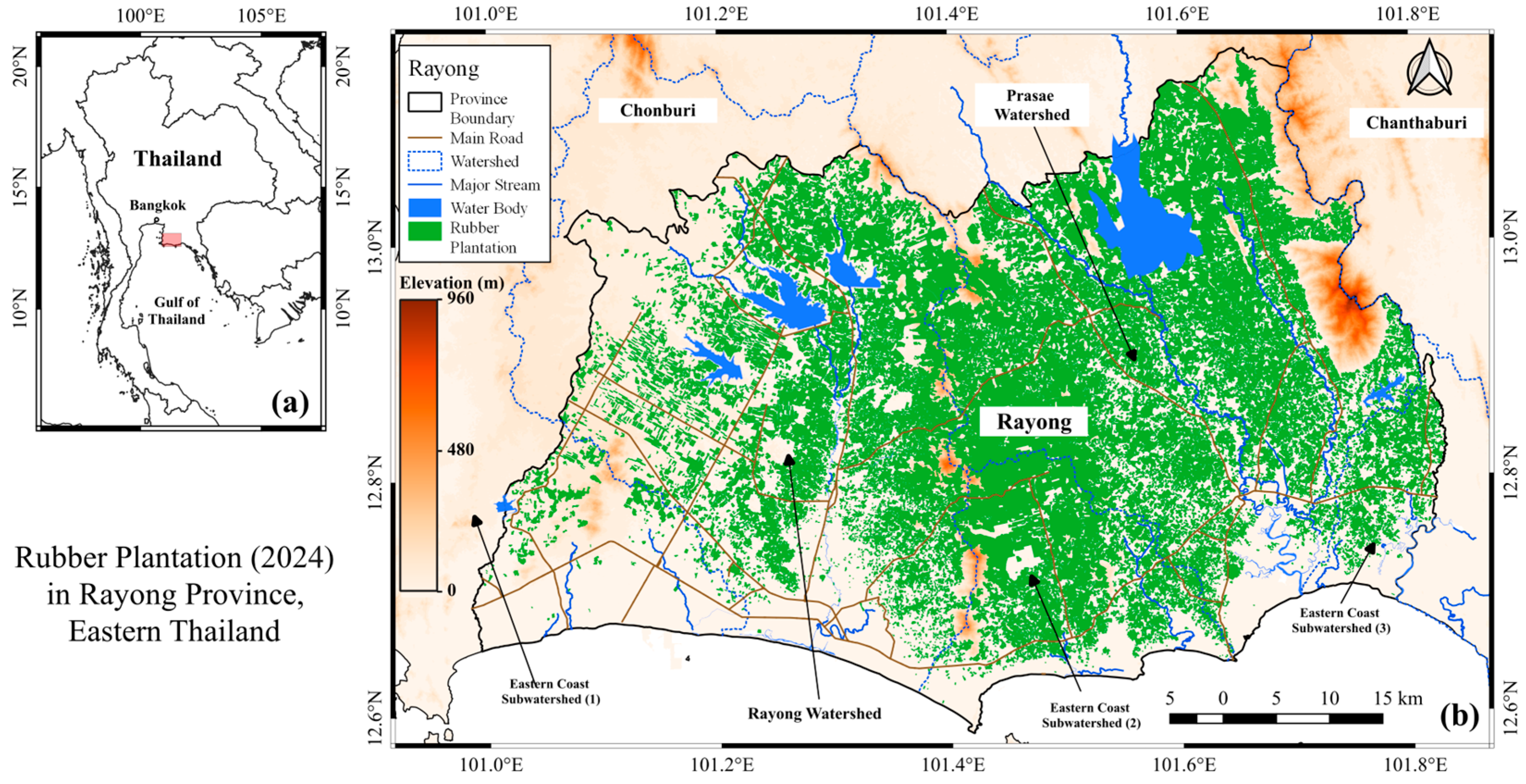
Figure 1. (a) Location of Rayong Province within Thailand; (b) Spatial distribution of rubber plantation areas in Rayong Province in 2024.
Forests 16 01652 g001
Figure 2. Workflow for pixel-based estimating tree and soil carbon stocks in rubber plantations. The top-left section is the process of mapping rubber plantation establishment years adopted from Wongsai et al. (2025) [26].
Forests 16 01652 g002
Figure 5. Cubic polynomial regression models with fixed intercepts for (a) diameter at breast height (DBH) and (b) height (H) of 360 sampled rubber trees aged between 5 and 27 years. Red lines represent the fitted regression curves for the predicted mean DBH and H values, while the shaded blue areas show the 95% confidence intervals for the expected mean response at each age. The fitted models are empirically constrained to the observed age range (5–27 years); values beyond this range are shown for visualization only and should be interpreted as illustrative extrapolations.
Forests 16 01652 g005
Figure 6. Estimated above-ground biomass (AGB) and below-ground biomass (BGB) of a rubber tree aged 3 to 33 years, calculated using allometric equations from three references: Witthawatchutikul and Jirasuktaveekul (1988) [44], Chiarawipa et al. (2024) [45], and Hytönen et al. (2018) [46]. Color bars represent model-specific AGB and BGB values.
Forests 16 01652 g006
Figure 7. Spatial distribution of estimated above- and below-ground carbon stock in rubber trees across Rayong Province in 2024, calculated using Hytönen et al. (2018) model and expressed in tonnes of carbon per 900 m2, corresponding to the pixel resolution.
Forests 16 01652 g007
Figure 8. Spatial distribution of (a) inherited and (b) changed SOC inventory in rubber plantations across Rayong Province in the year 2024. The map displays SOC stock in tonnes of carbon per pixel, derived from estimated changes following land conversion to rubber plantations.
Forests 16 01652 g008
Figure 9. Distribution of Δ SOC   by age group of the planation.
Forests 16 01652 g009
Table 1. Summary of predicted tree biomass in kilograms (kg) by the allometric model (n = 360 trees).
ModelMeanSDMedianIQRMin–Max
Witthawatchutikul and
Jirasuktaveekul (1998)
220.0122.9225.8208.715.9–502.2
Chiarawipa et al. (2024)242.4134.9241.2202.922.8–609.1
Hytönen et al. (2018)257.0159.3249.4238.315.0–715.5
SD = standard deviation; IQR = interquartile range.
Table 2. Total estimated carbon stock (in t C ha−1) of known age rubber trees in the study area, calculated using three different allometric models. The 95% confidence intervals were derived using the Delta Method based on uncertainty in DBH and height estimates.
Estimated MethodCarbon Stock
(t C ha−1)
95% Confidence
Interval (t C ha−1)
Relative Uncertainty
Witthawatchutikul and Jirasuktaveekul (1988)58.4053.59–63.73–8.2%, +9.1%
Chiarawipa et al. (2024)62.8055.77–69.83±11.2%
Hytönen et al. (2018)66.9458.19–75.69±13.1%
Totals reflect 82% of the plantation area with identified age.
Disclaimer/Publisher’s Note: The statements, opinions and data contained in all publications are solely those of the individual author(s) and contributor(s) and not of MDPI and/or the editor(s). MDPI and/or the editor(s) disclaim responsibility for any injury to people or property resulting from any ideas, methods, instructions or products referred to in the content.