Article

Positive Relationships Between Soil Organic Carbon and Tree Physical Structure Highlights Significant Carbon Co-Benefits of Beijing’s Urban Forests

College of Forestry, Beijing Forestry University, Beijing 100083, China
*
Author to whom correspondence should be addressed.
Forests 2025, 16(8), 1206; https://doi.org/10.3390/f16081206
Submission received: 12 June 2025 / Revised: 15 July 2025 / Accepted: 19 July 2025 / Published: 22 July 2025
(This article belongs to the Special Issue Ecosystem Services of Urban Forest)

Abstract

Increasing soil carbon storage is an important strategy for achieving sustainable development. Enhancing soil carbon sequestration capacity can effectively reduce the concentration of atmospheric carbon dioxide, which not only contributes to the carbon neutrality goal but also helps maintain ecosystem stability. Based on 146 soil samples collected at plot locations selected across Beijing, we examined relationships between soil organic carbon (SOC) and key characteristics of urban forests, including their spatial structure and species complexity. The results showed that SOC in the topsoil with a depth of 20 cm was highest over forested plots (6.384 g/kg–20.349 g/kg) and lowest in soils without any vegetation cover (5.586 g/kg–6.783 g/kg). The plots with herbaceous/shrub vegetation but no tree cover had SOC values in between (5.586 g/kg–15.162 g/kg). The plot data revealed that SOC was better correlated with the physical structure than the species diversity of Beijing’s urban trees. The correlation coefficients (r) between SOC and five physical structure indicators, including average diameter at breast height (DBH), average tree height, basal area density, and the diversity of DBH and tree height, ranged from 0.32 to 0.52, whereas the r values for four species diversity indicators ranged from 0.10 to 0.25, two of which were not statistically different from 0. Stepwise linear regression analyses revealed that the species diversity indicators were not very sensitive to SOC variations among a large portion of the plots and were about half as effective as the physical structure indicators for explaining the total variance of SOC. These results suggest that urban planning and greenspace management policies could be tailored to maximize the carbon co-benefits of urban land. Specifically, trees should be planted in urban areas wherever possible, preferably as densely as what can be allowed given other urban planning considerations. Protection of large, old trees should be encouraged, as these trees will continue to sequester and store large quantities of carbon in above- and belowground biomass as well as in soil. Such policies will enhance the contribution of urban land, especially urban forests and other greenspaces, to nature-based solutions (NBS) to climate change.

1. Introduction

With rapid urbanization, approximately 68% of the global population is expected to live in urban areas by 2050 [1]. Globally, over 70% of greenhouse gases (GHG) were emitted from urban areas [2], which only cover <1% of the Earth’s land surface [3]. In the meantime, carbon storage will be lost at an average rate of 9.3~12.9 Tg C yr−1 in 2010~2050 due to urban land expansion [4], making it quite challenging to achieve the target of carbon-neutral cities. Therefore, reducing urban greenhouse gas emissions must be considered as a core strategy for sustainable urban development [3]. Increasing carbon stock capacity in urban ecosystems will contribute to this strategy [5]. Conserving and developing green infrastructure is an efficient approach for increasing carbon sequestration over urban areas. As the main elements of nature-based solutions (NbS) to climate change [6,7,8,9], urban forests provide significant carbon sequestration capacity [10]. It has been reported that carbon sequestration by urban trees and green spaces can be high in residential environments [11,12,13]. In addition to the aboveground biomass stored in trees and other vegetation types, urban soil can provide long-term storage for sequestered carbon. It has been demonstrated that as much as 64% of urban carbon could be contributed by soil carbon [14]. While increasingly more efforts are devoted to the study of urban soil carbon at multiple scales, the impact of urban green and blue infrastructure on soil carbon is not well understood [15].
For natural forest and grassland ecosystems, there has been a growing recognition that carbon sinks are often influenced by complex species and structural diversity [16]. But the relative contributions of spatial structure and species diversity to forest carbon storage capacity remain a key scientific issue to be clarified [17,18]. For instance, the carbon allocation mechanism of ecosystems is significantly related to the spatial structure of forest stands, but the determining factor of the upper limit of ecosystem carbon stock points to species diversity [19].
Previous studies have suggested that relationships exist between carbon pools and stand spatial structure [20,21]. The intensity of isolation and the distribution and competition of trees have a profound effect on forest productivity and carbon sequestration strength [22,23]. The stability and growth potential of trees, as well as the intensity of competition between adjacent trees, are all affected by forest structure [24,25,26]. Therefore, the spatial structure of forest stands ultimately determines the quality of their conditions, which affects their carbon sequestration capacity.
It was proposed that species diversity has a decisive impact on the stability and productivity of ecosystems [27]. For grassland ecosystems, soil organic carbon was strongly affected by the Shannon index [28]. The higher the species richness, the stronger the carbon sequestration capacity by soil [29,30]. It has been demonstrated that plant communities with high species richness had higher productivity and stronger long-term soil organic carbon (SOC) storage capacity [31]. Nonetheless, some researchers believed that the interaction mechanisms between carbon sequestration capacity and species diversity in forest ecosystems were still ambiguous due to the disunity of scales. This was at the heart of the current debate about relationships between carbon sequestration capacity and species diversity [32].
For urban ecosystems, less attention has been devoted to understanding the relationships between soil carbon and forest structure and species composition, although the carbon storage or carbon sequestration capacity of urban vegetation has been subject to many studies. For example, the effects of green space types [33,34], urban forest types (e.g., coniferous, broadleaved, and mixed forest) [35], and vegetation in urban, suburban, and peri-urban forests [36] on soil carbon have been investigated through field experiments or sample-based local studies. At the city or regional scales, remote sensing data have been utilized to study the influences of land use change [37], vegetation index as a surrogate of vegetation cover [38], and impermeable ground cover [39] on soil carbon. Relationships between urban soil carbon and the spatial structure and species composition of urban forests have yet to be investigated.
Urban forests differ from natural and plantation forests in many ways. For many practical reasons, for example, woody plant richness in urban forests is often very low [40], because typically only selected tree species are planted in most local neighborhoods. Urban trees are often subject to pruning, fertilization, litter cleaning, and other management practices specific to urban areas [41]. Given these differences, we hypothesized that the relative impacts of stand structure and species composition on SOC in urban environments might be different from those observed in previous studies of natural or plantation forests. The main purpose of this study is to test this hypothesis by examining the relative relationships between SOC and two key aspects of urban forests, including stand structure and species composition, through a case study conducted in Beijing. A good understanding of such relationships is needed for developing urban forest management practices that enhance urban soil carbon sequestration, which will ultimately contribute to the development of sustainable, carbon-neutral urban growth pathways.

2. Materials and Methods

2.1. Study Area

This study was conducted over the area within the 6th Ring Road of Beijing (Figure 1). With a total area of 16,410.54 km2, Beijing is centered at approximately 39°56′ N, 116°20′ E. The entire administrative region of Beijing is characterized by higher elevations in the northwest and lower elevations in the southeast, with the Beijing Plain in the middle. Our study area is located entirely within the Beijing Plain, which is surrounded by mountains in the west, north, and east, with gently sloping terrains in the southeast [42]. By the end of 2023, the city’s resident population was 2.1843 × 10⁷. It had a forest coverage rate of 44.9% and a stock volume of 40.78 × 10⁶ m3. The green coverage rate was 49.8% in the built area. Beijing belongs to a semi-humid and semi-arid monsoon climate in the warm temperate zone, with an average annual temperature of 10~12 °C and an average annual precipitation of about 600~620 mm. It has hot and humid summers, cold and dry winters, and relatively short spring and autumn seasons [43].
Fluvo-aquic and cinnamon soils are the major soil types over the study area, covering approximately 70% and 20% of the plain areas of Beijing, respectively [42]. Fluvo-aquic soils were formed with Holocene alluvial parent materials and primarily comprised of loamy soils, luvic soils, and sandy soils [42]. Cinnamon soils are predominantly distributed in piedmont plains with elevations above 40 m. The soils in the urban built-up areas generally exhibit alkaline properties [44], with pH values over 8.0 on average and higher in certain localized regions [45]. With a bulk density varying between 0.96 and 1.67 g/cm3, the soils have total nitrogen contents ranging from 0.23 to 2.46 g/kg [46]. Other soil nutrient concentrations in the main urban areas of Beijing exhibited the following ranges: alkali-hydrolyzable nitrogen (AN) from 3.50 to 159.61 mg/kg, available phosphorus (AP) from 11.34 to 36.15 mg/kg, and available potassium (AK) from 56.88 to 491.17 mg/kg [47].

2.2. Field Data Collection

The data used in this study were collected in May 2023 over sample locations distributed across the area located within Beijing’s 6th Ring Road (Figure 1). The sample locations were selected using the following method. First, we designed a geographical grid at an interval of 2 km × 2 km, and we took the urban center point as the origin of the grid system. Then, we designed 8 fan-shaped transects from the origin to the 6th Ring Road. The transects had equal angular intervals in 8 directions (Figure 1). Because many major streets in Beijing follow east-west or north-south directions, to minimize any potential impact of spatial autocorrelation issues, the 8 transects were rotated slightly and synchronously away from the north-south and east-west directions such that they did not align with the directions of those main streets perfectly. Finally, the grid points located within the fan-shaped transects were selected as sampled plots. In total, 146 plots were selected. Each plot had an area of 30 m × 30 m (Figure 1).
At each plot location, trees with diameter at breast height (DBH) ≥ 4 cm were tallied. Key information recorded for each tree included species name, DBH, tree height, branching height, crown width, etc. It should be noted that although DBH and tree height are often used to estimate aboveground biomass, they were not used that way in this study because Beijing’s forest biomass has been studied previously [48,49]. Rather, those measurements were used to examine relationships between soil organic carbon and vegetation structure (see Section 2.4). A total of 2564 trees were recorded in the study area, with Styphnolobium japonicum being the most abundant species (Table A1), followed by Populus tomentosa and Pinus tabuliformis. The shrub layer was dominated by Buxus megistophylla, while the herbaceous layer was primarily composed of Crepidiastrum sonchifolium (see detailed shrub and herb data in Table A2 and Table A3, respectively).
At each plot location, a soil auger was used to collect topsoil cores (with a depth of 20 cm) following the five-point sampling method. With this method, soil cores were taken at 5 points within each sample plot. The five points were arranged such that they formed a cross centered at the center of each plot. For each plot location, we first mixed the soil samples collected at the five points thoroughly, reduced the weight to approximately 500 g using the four-part method, and then packed the 500 g of soil in a clean bag for lab analysis [50]. For plots dominated by street trees, topsoil was collected by randomly selecting five adjacent street trees and using the soil auger to collect the topsoil core within each tree pit. The soil samples were air-dried in a cool, dry room. Gravel and roots were removed using a 2 mm full-aperture sieve followed by screening using a 100-mesh sieve. Soil organic carbon was determined using the potassium dichromate oxidation-dilution heat method [50,51].

2.3. Calculation of Plot-Level Species Complexity and Forest Spatial Structure Indicators

The indicators used in this study were selected based on previous studies (Table 1). Specifically, we used average diameter at breast height (DA), average tree height ( H ¯ ), basal area density (i.e., basal area per hectare, G), and the diversity of DBH (DDBH) and tree height (DTH) to express the complexity of the physical structure of a forest stand and used the Margalef richness index (SR), Shannon–Wiener index (H), Pielou evenness (E), and Berger–Parker dominance (DBP) to represent the complexity of species composition. Equations and full definitions of these indicators are provided in Table 1.

2.4. Data Analysis

With the data collected over the 146 plot locations, we first calculated the mean and standard deviation of SOC for different soil and vegetation types to examine whether and how SOC content might differ among those types. For the forested plots, we also calculated SOC mean and standard deviation values for plots with different understory compositions to evaluate the impact of understory composition on SOC. We used the Kruskal-Wallis method to examine the significance (p-value) of among-group differences [56].
To examine the relationships between SOC and the 9 indicators calculated in Section 2.3 (Table 1), we calculated the Spearman correlation coefficient (r) for each indicator pair and between SOC and each of those indicators. To estimate the amount of SOC variance explained by different variable groups (R2), we developed stepwise linear regression models between SOC and the 5 physical structure indicators, 4 species diversity indicators, and both. As will be shown later (see Section 3.2), some of the indicators were highly correlated with one another. Stepwise linear regression can help identify collinearity issues and only use predictors that are statistically significant.

3. Results

3.1. SOC Distribution by Soil and Vegetation Types

The SOC values over Beijing, as represented by the 146 sample plots, ranged from 5.586 g/kg to 20.349 g/kg, which are within the range reported for Beijing in a previous study [46]. The dominant soil types sampled through this study were loamy (62.8%) and sandy soils (35.4%, Table A4), which had average SOC of 11.922 g/kg and 11.367 g/kg, respectively. A tiny fraction (1.8%) of the collected samples had the clay soil type, which had a slightly higher mean SOC value of 13.965 g/kg. Statistically, however, no significant difference existed among the SOC values of the three soil types (Figure 2).
Over 90% of the sample locations had forest cover, including 58.4% broadleaved forest plots, 3.8% coniferous forest plots, and 33% mixed forest plots (Table A4). Of the 10 plots that had no tree cover, 6 had shrub and/or herbaceous plants, and 4 had no vegetation cover. The 4 non-vegetated plots had a mean SOC value of 5.885 g/kg, while the average value of the 6 non-forested plots that had herbaceous and/or shrub cover was 8.712 g/kg (Figure 3, left). The SOC of the forested plots ranged from 6.384 g/km to 20.349 g/kg, which were significantly higher than those of the two non-forest plot types. Among the forested plots, neither forest type nor understory cover had a statistically significant impact on SOC contents. The average SOC values for plots with coniferous, broadleaved, and mixed forests were 12.768 g/kg, 11.934 g/kg, and 12.231 g/kg, respectively (Figure 3, left). About half (53.2%) of the forested plots had both shrub and herb layers, and plots that had only herbaceous vegetation, shrubs, or neither accounted for 28%, 8.8%, and 11%, respectively (Table A4). The average SOC values for the forested plots with herbaceous understory, shrub understory, both, and neither were 12.004 g/kg, 11.888 g/kg, 11.965 g/kg, and 10.150 g/kg, respectively (Figure 3, right).

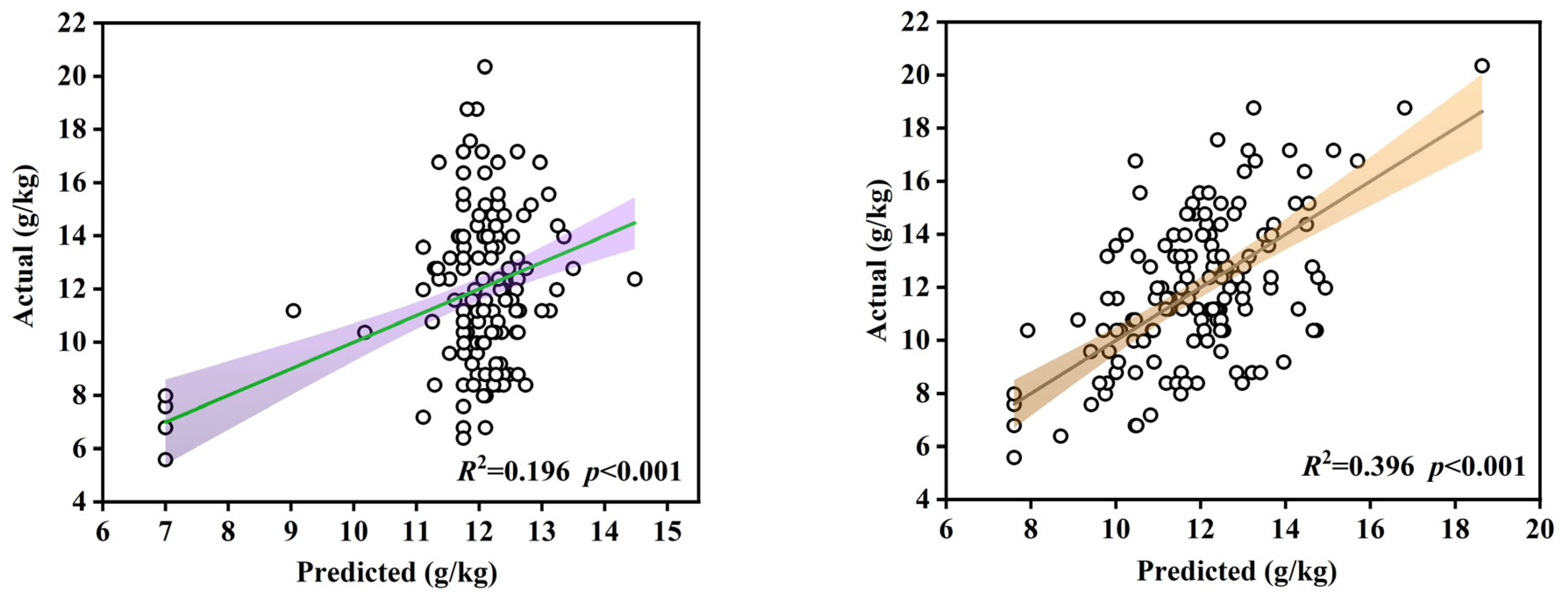
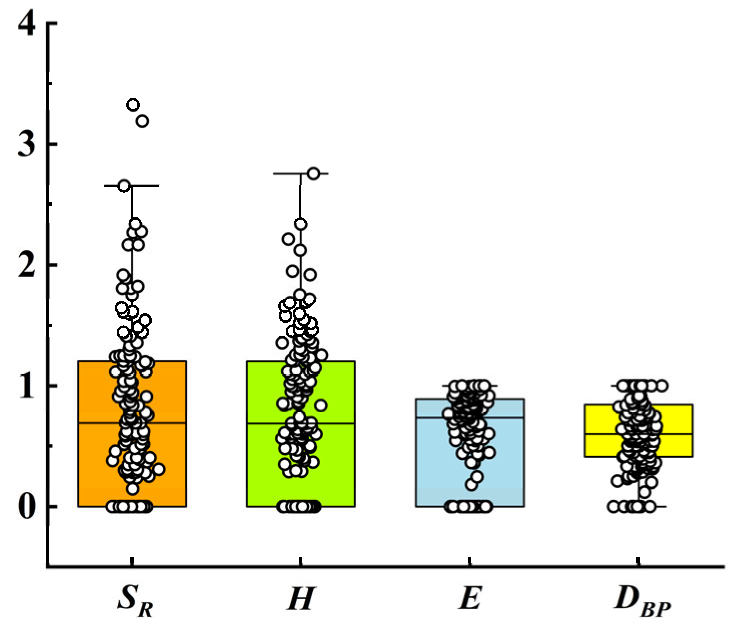
3.2. Relationships Between SOC and Forest Structure and Species Diversity Indicators

Overall, SOC had good correlations with the physical structure indicators (Figure 4). The correlation coefficient was highest between SOC and G, basal area density, followed by those between SOC and average tree height ( H ¯ ), average DBH (DA), diversity of DBH (DDBH), and diversity of tree height (DTH). Ranging from 0.32 to 0.52, these correlation coefficient values were all statistically different from 0 with p < 0.001. The species diversity indicators, however, were less correlated with SOC. Of the four indicators considered in this study, only the Shannon–Wiener diversity (H) and Margalef species richness (SR) indices were significantly correlated with SOC (p < 0.05). The correlation coefficient values between SOC and the other species diversity indicators (i.e., E and DBP) were not statistically different from 0 at the 95% confidence level (p > 0.05) (Figure 4).
As expected, multiple indicators explained more SOC variance than individual indicators. Given that many indicators were highly correlated with one another (Figure 4), only some of them were selected as statistically significant predictors by the stepwise linear regression (SLR) method. For the 4 species diversity indicators, only the Shannon–Wiener Diversity (H) and Berger–Parker Dominance (DBP) were selected as statistically significant predictors (p < 0.05). Together, the two indicators explained almost 20% of the total variance of SOC (Table 2). When the 5 structure indicators were used as predictors, only 3 of them were selected, including the diversity of DBH (DDBH), basal area density (G), and average tree height ( H ¯ ). Together, they explained about 40% of the total variance of SOC. Interestingly, the same 3 structure indicators were selected by SLR when the 4 species diversity indicators and 5 structure indicators were used together as predictor variables, indicating that given the 5 structure indicators, the species diversity indicators were redundant for SOC prediction.
A comparison of SOC predicted using different SLR models and field measurements at individual plot locations revealed that the model based on the species diversity indicators had low sensitivity to SOC variations. Figure 5 (left) shows that a large number of plots had predicted values within a narrow range between 11 g/kg and 13 g/kg, but their actual values varied from 6 g/kg to 20 g/kg. The model based on the physical structure indicators was much better for SOC prediction. Its predictions had a value range close to that of the field measurements, and the distributions of the plots within the predicted value range and the value range of the field measurements were similar (Figure 5, right).

4. Discussion

Soil is an important carbon pool, storing more carbon than vegetation biomass in most terrestrial ecosystems [57]. However, there are many challenges to soil carbon estimation, especially over large areas [58], and current understanding of soil carbon dynamics is highly uncertain [59]. While both vegetation structure and species diversity have been explored as indicators of soil organic carbon [27,28,29,30,31], this study demonstrated that tree physical structure was better correlated with SOC than species diversity in urban areas. Our results highlight an important carbon sink in urban soil and may provide a theoretical basis for developing tree-based urban planning and greenspace management policies that can maximize the carbon co-benefits of urban land.

4.1. Effectiveness of Tree Structure Measurements as Indicators of SOC in Urban Areas

While many studies demonstrated that SOC was positively related to species diversity over natural forest [28,29,30,60,61] and grassland areas [28,60], Xu et al. [35] showed that diameter at breast height was the best predictor of urban SOC among all the forest properties considered in that study. The field data collected through this study demonstrated that physical structure properties of urban forests were much better indicators of SOC than species diversity. The correlation coefficient values between SOC and five physical structure indicators calculated based on tree diameter and height measurements were much higher than those between SOC and four species diversity indicators. Stepwise linear regression analyses revealed that the amount of SOC variance explained by the physical structure indicators was twice as much as that explained by the species diversity indicators. While the latter seemed to be able to explain almost 20% of the total SOC variance, they had very low sensitivity to SOC variations for the majority of the sample plots. The predicted SOC of those plots by the species diversity indicators had a value range (11 g/kg–13 g/kg) much narrower than that of the field measurements (6 g/kg and 20 g/kg) (Figure 5, left). Further, none of the species diversity indicators had statistically significant contributions to SOC prediction when they were used together with the physical structure indicators as predictor variables in stepwise linear regression analyses.
A tree’s physical structure can be linked to SOC in several ways. First, tree diameter and height are among the best predictors of aboveground biomass. Many allometric equations for biomass estimation are based on DBH alone or a combination of DBH and height [62,63]. According to those equations, large and/or tall trees have high aboveground biomass values and hence high belowground biomass [64], which contributes to SOC. Also, SOC in deep soil is tightly linked to root processes [65]. Large trees typically have complex root systems that can distribute biomass carbon in deep soils over areas larger than the areas covered by the crowns of those trees, even when those areas were covered by pavements [66]. Further, most large trees are very old, which represents long histories of carbon input to the soil through litter, understory vegetation, and/or fertilization, which should also contribute to increased SOC [67,68].
The weak relationships between SOC and the species diversity indicators as observed in this study might be attributed to the fact that tree species composition in urban areas was relatively simple, especially at the plot scale. About 20% of the plots used in this study had a single tree species, and over 30% of the plots had 2 tree species. For the entire study area, over 26% and a quarter of sampled plots had SR and H values less than 0.2, respectively (Figure A1). The median values of SR, H, E, and DBP were 0.692, 0.689, 0.746, and 0.600, respectively (Figure 6), which were low but were in accordance with those reported by Ma & Jia [69]. Lack of high levels of species diversity likely contributed to the weaker than expected relationships between species diversity indicators and SOC.
It should be noted that although soil substrate, forest type, and understory vegetation are among the many factors that could shape the distribution of SOC, it does not appear those factors had any major impact on the relative effectiveness of the tree physical structure and species diversity indicators considered in this study for SOC prediction. Except for the few non-vegetated plots that had significantly lower SOC contents, no statistically significant differences were found among the mean SOC values for different soil types, forest types, or different types of understory cover (Figure 2 and Figure 3). Of course, SOC in urban forests is affected by many factors, including substrate and soil type, litter input [70,71], soil microbe community [72], soil nitrogen [67,73], vegetation type, structure, and age [67,68], as well as the presence of shrubs [74] and herbaceous cover [75]. The relationships demonstrated in this study may not be robust enough for accurate prediction of SOC across Beijing. More factors should be considered in order to develop better SOC prediction models over urban areas.

4.2. Urban Soil as a Significant Carbon Sink

Urban land is very important for human society, providing living space for more than half of the global population [1]. While accounting for a small fraction of the Earth’s land surface, global urban area will continue to increase due to development and rapid population growth [3]. Although urban land expansion generally leads to carbon storage loss [4], significant carbon sequestration can also be achieved over human settlement areas. In the conterminous United States (CONUS), for example, human settlements could store as much carbon per unit area as tropical forests, and the total carbon storage in those areas accounted for 10% of the total land carbon storage across CONUS, including 64% in soil, 20% in vegetation, 11% in landfills, and 5% in buildings [14]. For a typical city in the U.K., 82% of organic carbon was held in soils, including 13% found under impervious surfaces, and 18% was stored in vegetation [39]. Obviously, soil is a dominant carbon pool over urban areas. Other major carbon pools in urban areas include urban vegetation and built-up structures, especially wooden buildings [12].
Urban soil can provide carbon storage over a very long time. Substantial “hidden” carbon may be stored in subsoils, cultural layers, and sealed soils beneath impervious surfaces. While some argued that SOC stocks in natural habitats were higher than those of urban green spaces and urban intensive habitats [76], it was demonstrated that urban soil carbon storage could be significantly greater than agricultural land [39] in certain regions. Another study showed that the total C content in urban soils was 1.5–3 times higher for a wide range of climatic conditions, and C accumulation was much deeper compared with natural soils [77]. Because urban soils, especially those covered by impervious surfaces, are less likely to be disturbed than agricultural soils, they can store carbon for much longer than agricultural and forest soils. As global urban areas continue to increase rapidly [3], so will the importance of urban soil as a carbon sink.

4.3. Implications for Urban Planning and Greenspace Management

The positive relationships between SOC and forest structure have important implications regarding urban planning and greenspace management. Greenspaces are important urban fabrics designed to promote health and well-being in cities [78]. In addition to the wide range of services they can provide, including many societal, air quality, and microclimatic benefits; ecosystem protection; flood mitigation; and landscape beautification [79], among others, urban trees also have significant carbon co-benefits. They sequester and store large quantities of carbon in biomass and soil. Our study results demonstrated that most areas with non-forest vegetation cover or no vegetation cover have lower SOC values than forested areas, and structurally complex urban trees are typically associated with high SOC.
It should be noted that only soils in the top 20 cm were considered in this study. Given that large trees have deep roots that often extend horizontally to encompass areas several times larger than the areas covered by the crowns of those trees [80], SOC differences between forested plots and nonforest plots in soils beyond the 20 cm depth likely will be larger than those reported for the topsoil, meaning the carbon co-benefits of urban forests in deep soils likely will be larger than shown in this study. Therefore, urban tree management policies should be designed to promote the growth and preservation of mature, structurally complex urban trees and forests. Where possible, trees should be planted with adequate densities in order to increase basal area, which is better correlated with SOC than any of the other structure indicators considered in this study. Given that litter removal in urban areas is often necessary for urban beautification and other practical purposes, innovative litter disposal methods are needed to keep litter carbon from being released to the atmosphere for as long as possible. Successful implementation of such policies is crucial for including urban land, especially urban forests and other greenspaces, as an integral part of nature-based solutions (NBS) to climate change [8].

5. Conclusions

This study examined relationships between soil organic carbon (SOC) and key characteristics of urban forests, including their spatial structure and species complexity. According to 146 soil samples collected at plot locations selected from the urban area surrounded by Beijing’s 6th Ring Road, SOC in the topsoil with a depth of 20 cm in Beijing was highest over forested plots, ranging from 6.384 g/kg to 20.349 g/kg, while soils without any vegetation cover had the lowest SOC, ranging from 5.586 g/kg to 6.783 g/kg. The plots with herbaceous/shrub vegetation but no tree cover had SOC values in between, ranging from 5.586 g/kg to 15.162 g/kg. While good relationships between SOC and vegetation species diversity were observed over natural forest and grassland areas in previous studies, our results showed that SOC was better correlated with the physical structure than the species diversity of Beijing’s urban trees. Specifically, SOC had positive, statistically significant correlations with five physical structure indicators, including average DBH, average tree height, basal area density, and the diversity of DBH and tree height, with correlation coefficients (r) ranging from 0.32 to 0.52. Correlations between SOC and four species diversity indicators were much weaker, with r values ranging from 0.10 to 0.25, two of which were not statistically different from 0. Stepwise linear regression analyses revealed that the species diversity indicators were not very sensitive to SOC variations among a large portion of the plots and could only explain half of the SOC variance explained by the physical structure indicators.
These results may provide a theoretical basis for developing tree-based urban planning and greenspace management policies with a goal to maximize the carbon co-benefits of urban land. Specifically, trees should be planted in urban areas wherever possible, preferably as densely as what can be allowed given other urban planning considerations. This will result in high basal area densities, which had the best correlations with SOC among the indicators considered in this study. Protection of large, old trees should be encouraged, as these trees will continue to sequester and store large quantities of carbon in above- and belowground biomass as well as in soil. Such policies will enhance the contribution of urban land, especially urban forests and other greenspaces, to nature-based solutions (NBS) to climate change [8].

Author Contributions

R.X., S.M.H.S., C.X., and S.L. conceived the idea for this study. R.X., S.M.H.S., C.X., X.L., and B.M. were investigated and sampled together. R.X. analyzed the data and wrote the first draft of the paper. S.M.H.S., C.X., X.L., S.L., and B.M. contributed to the writing through multiple rounds of revisions. C.X. helped the team obtain funding, provided the resources needed for the research, and made important contributions to the improvement of research methods. C.X. and S.L. supervised and led the entire study. All authors have read and agreed to the published version of the manuscript.

Funding

This research was funded by 5·5 Engineering Research & Innovation Team Project of Beijing Forestry University grant number BLRC2023B06.

Data Availability Statement

The research content of this paper has not yet been concluded, and the original data will be kept confidential for the time being.

Acknowledgments

The authors are grateful for the support from the 5.5 Engineering Projects. The authors would like to express their heartfelt thanks to Xuan Guo, Yang Li, Parsa Mushtaq, Murtaza Ali, Xian Shi, Yupei Xu, Jiaxin Guo, Qian Xiao, Zuoyou Hu, Zhihui Yang, and Jialin Dong for their help in the data investigation of the article.

Conflicts of Interest

The authors declare that they have no known competing financial interests or personal relationships that could have appeared to influence the work reported in this paper.

Appendix A

Table A1. Statistical table of trees measured in this study.
Tree Species Name (Scientific Name)FamilyProportion
(%)
Styphnolobium japonicum Fabaceae 12.52
Populus tomentosa Salicaceae 11.00
Pinus tabuliformis Pinaceae 8.70
Ginkgo biloba Ginkgoaceae 7.53
Salix matsudana Salicaceae 5.15
Ailanthus altissima Simaroubaceae 4.72
Fraxinus pennsylvanica Oleaceae 3.98
Juniperus chinensis Cupressaceae 3.74
Fraxinus velutina Oleaceae 3.39
Eucommia ulmoides Eucommiaceae 2.77
Prunus cerasifera ‘Atropurpurea’ Rosaceae 2.65
Robinia pseudoacacia Fabaceae 2.50
Koelreuteria paniculata Sapindaceae 2.38
Platycladus orientalis Cupressaceae 2.34
Platanus acerifolia Platanaceae 2.30
Malus spectabilis Rosaceae 2.11
Cedrus deodara Pinaceae 1.95
Acer truncatum Sapindaceae 1.83
Ulmus pumila Ulmaceae 1.76
Echeveria ‘Peach Pride’ Rosaceae 1.21
Salix babylonica Salicaceae 1.17
Pinus bungeana Pinaceae 1.05
Platanus occidentalis Platanaceae 0.94
Juglans regia Juglandaceae 0.74
Platanus orientalis Platanaceae 0.70
Acer pictum subsp. mono Sapindaceae 0.70
Toona sinensis Meliaceae 0.62
Prunus sibirica Rosaceae 0.59
Yulania denudata Magnoliaceae 0.55
Lonicera maackii Caprifoliaceae 0.55
Aesculus chinensis Sapindaceae 0.55
Prunus triloba Rosaceae 0.47
Broussonetia papyrifera Moraceae 0.43
Populus nigra Salicaceae 0.43
Quercus mongolica Fagaceae 0.39
Sabina chinensis Cupressaceae 0.35
Prunus davidiana Rosaceae 0.31
Morus alba Moraceae 0.27
Pyrus communis Rosaceae 0.27
Yulania denudata Magnoliaceae 0.23
Prunus serrulata Rosaceae 0.23
Crataegus pinnatifida Rosaceae 0.20
Amorpha fruticosa Fabaceae 0.20
Populus nigra Salicaceae 0.20
Lagerstroemia indica Lythraceae 0.20
Pinus armandii Pinaceae 0.20
Acer tataricum subsp. ginnala Sapindaceae 0.20
Juniperus formosana Cupressaceae 0.20
Picea asperata Pinaceae 0.20
Prunus cerasifera Rosaceae 0.16
Euonymus maackii Celastraceae 0.16
Malus pumila Rosaceae 0.16
Prunus serrulata Rosaceae 0.16
Paulownia fortunei Paulowniaceae 0.16
Prunus persica ‘Atropurpurea’ Rosaceae 0.16
nectarine Rosaceae 0.16
Populus canadensis Salicaceae 0.12
Prunus pseudocerasus Rosaceae 0.12
Pinus parviflora Pinaceae 0.12
Morus nigra Moraceae 0.12
Prunus persica Rosaceae 0.08
Acer palmatum Sapindaceae 0.08
Fraxinus rhynchophylla Oleaceae 0.08
Ziziphus jujuba Rhamnaceae 0.08
Styphnolobium japonicum ‘Pendula’ Fabaceae 0.08
Cotinus coggygria Anacardiaceae 0.08
Syringa oblata Oleaceae 0.08
Taxus wallichiana Taxaceae 0.08
Pyrus pyrifolia Rosaceae 0.08
Diospyros kaki Ebenaceae 0.08
Picea wilsonii Pinaceae 0.04
Table A2. Statistical table of shrub layer plants in the survey area.
Shrub Layer Species Name (Scientific Name)Quantity of Sample PlotsShrub Layer Species Name (Scientific Name)Quantity of Sample Plots
Buxus megistophylla 23 Jasminum nudiflorum 2
Broussonetia papyrifera 16 Lagerstroemia indica 2
Rosa chinensis 11 Malus micromalus 2
Lonicera japonica 10 Juniperus sabina 2
Buxus sinica 9 Rosa xanthina 2
Ulmus pumila 8 Viburnum acerifolium 1
Morus alba 6 Jasminum mesnyi 1
Styphnolobium japonicum 6 Berberis amurensis 1
Forsythia suspensa 6 Berberis thunbergii ‘Atropurpurea’ 1
Juniperus procumbens 6 Metaplexis hemsleyana 1
Ailanthus altissima 5 Euonymus fortunei 1
Toona sinensis 5 Averrhoa carambola 1
Cercis chinensis 4 Rhamnus leptophylla 1
Ligustrum vicaryi 4 Prunus serrulata 1
Syringa oblata 4Koelreuteria paniculata1
Prunus triloba 4 Ziziphus jujuba 1
Ligustrum ovalifolium 3 Weigela florida 1
Echeveria ‘Peach Pride’ 3 Paulownia tomentosa 1
Ligustrum quihoui 3 Amorpha fruticosa 1
Prunus persica ‘Atropurpurea’ 3 Juglans regia 1
Ginkgo biloba 3 Platycladus orientalis 1
Populus tomentosa 3 Robinia pseudoacacia 1
Prunus cerasifera ‘Atropurpurea’3Pyrus communis1
Lespedeza chinensis 2 Prunus padus 1
Ilex chinensis 2 Sabina chinensis 1
Kerria japonica 2 Tilia tuan 1
Juniperus chinensis 2 Chimonanthus praecox 1
Hibiscus syriacus 2 Fraxinus pennsylvanica 1
Vitex negundo 2
Table A3. Statistical table of herbaceous layer plants in the survey area.
Herbaceous Layer Species Name (Scientific Name)Quantity of Sample PlotsHerbaceous Layer Species Name (Scientific Name)Quantity of Sample Plots
Crepidiastrum sonchifolium 45 Abutilon theophrasti 2
Chenopodium album 38 Oxalis corniculata 2
Ophiopogon japonicus 26 Acalypha australis 2
Setaria viridis 23 Dodonaea viscosa 1
Taraxacum mongolicum 22 Veronica persica 1
Viola arcuata 14 Trigonotis peduncularis 1
Lolium perenne 14 Calamintha debilis 1
Humulus scandens 12 Medicago sativa 1
Plantago asiatica 9 Ligustrum lucidum 1
Potentilla supina 8 Imperata cylindrica 1
Lepidium apetalum 8 Nepeta cataria 1
Poa annua 7 Cervus canadensis 1
Artemisia argyi 7 Cirsium vlassovianum 1
Cirsium arvense 7 Ixeris chinensis 1
Hosta plantaginea 5 Lythrum salicaria 1
Digitaria sanguinalis 5 Chloris virgata 1
Iris tectorum 5 Vincetoxicum chinense 1
Artemisia annua 5 Vallisneria natans 1
Inula japonica 4 Oenothera biennis 1
Potentilla chinensis 4 Hedyotis auricularia 1
Calystegia hederacea 4 Melica scabrosa 1
Rubia cordifolia 4 Artemisia mongolica 1
Hemerocallis fulva 4 Prunella vulgaris 1
Eleusine indica 4 Hemisteptia lyrata 1
Duchesnea indica 3 Rumex crispus 1
Phyllostachys edulis 3 Cynanchum bungei 1
Hemerocallis citrina 3 Ipomoea nil 1
Iris lactea 3 Elymus kamoji 1
Bassia scoparia 3 Aster hispidus 1
Convolvulus arvensis 3 Leptopus chinensis 1
Carex duriuscula 3 Ceratopteris thalictroides 1
Lespedeza bicolor 3 Solanum nigrum 1
Ophiopogon bodinieri 3 Galinsoga quadriradiata 1
Persicaria lapathifolia 3 Eriochloa villosa 1
Erigeron canadensis 2 Impatiens balsamina 1
Orychophragmus violaceus 2 Capsella bursa-pastoris 1
Phragmites australis 2 Arabidopsis thaliana 1
Gaillardia pulchella 2 Alternanthera philoxeroides 1
Artemisia capillaris 2 Tragopogon orientalis 1
Zea mays 2 Rehmannia glutinosa 1
Saussurea japonica 2 Plantago depressa 1
Lactuca indica 2 Paederia foetida 1
Cynodon dactylon 2 Cosmos bipinnatus 1
Adiantum capillus-veneris 2 Klasea centauroides 1
Sonchus oleraceus 2 Ipomoea purpurea 1
Bothriospermum chinense 2 Acorus calamus 1
Table A4. Distribution of forest types, understory composition, and soil types among the sample locations.
Forest typesProportion of sampling plots (%)
No tree4.5
Coniferous forest3.8
Broadleaved forest58.4
Mixed coniferous and broadleaved forest33.0
Understory compositionProportion of sampling plots (%)
No vegetation under the forest11
Only herbaceous plants in the understory28
Only shrubs in the understory8.8
The understory had both shrubs and herbaceous vegetation 53.2
Soil typeProportion of sampling plots (%)
Sandy soil35.4
Loamy soil62.8
Clay1.8
Figure A1. Frequency distribution of different classes of woody plant composition indices values. We divided values of four diversity indices by 0.2 intervals, and all of the values bigger than 2.0 are included in the class >2.0, because fewer values of diversity indices were bigger than 2.0. SR, Margalef species richness; H, Shannon–Wiener index; E, Pielou evenness; DBP, Berger–Parker Dominance.
Forests 16 01206 g0a1

References

  1. United Nations Department of Economic and Social Affairs (UN DESA). The 2018 Revision of the World Urbanization Prospects 2018. Available online: https://www.un.org/zh/desa/68-world-population-projected-live-urban-areas-2050-says-un (accessed on 16 May 2018).
  2. Zhao, D.; Cai, J.; Xu, Y.; Liu, Y.; Yao, M. Carbon Sinks in Urban Public Green Spaces under Carbon Neutrality: A Bibliometric Analysis and Systematic Literature Review. Urban For. Urban Green. 2023, 86, 128037. [Google Scholar] [CrossRef]
  3. Xu, W.; Wang, G.; Liu, S.; Wang, J.; McDowell, W.H.; Huang, K.; Raymond, P.A.; Yang, Z.; Xia, X. Globally Elevated Greenhouse Gas Emissions from Polluted Urban Rivers. Nat. Sustain. 2024, 7, 938–948. [Google Scholar] [CrossRef]
  4. Liu, X.; Wang, S.; Wu, P.; Feng, K.; Hubacek, K.; Li, X.; Sun, L. Impacts of Urban Expansion on Terrestrial Carbon Storage in China. Environ. Sci. Technol. 2019, 53, 6834–6844. [Google Scholar] [CrossRef] [PubMed]
  5. Esperon-Rodriguez, M.; Tjoelker, M.G.; Lenoir, J.; Baumgartner, J.B.; Beaumont, L.J.; Nipperess, D.A.; Power, S.A.; Richard, B.; Rymer, P.D.; Gallagher, R.V. Climate Change Increases Global Risk to Urban Forests. Nat. Clim. Change 2022, 12, 950–955. [Google Scholar] [CrossRef]
  6. Jiang, Y.; Sun, Y.; Liu, Y.; Li, X. Exploring the Correlation between Waterbodies, Green Space Morphology, and Carbon Dioxide Concentration Distributions in an Urban Waterfront Green Space: A Simulation Study Based on the Carbon Cycle. Sustain. Cities Soc. 2023, 98, 104831. [Google Scholar] [CrossRef]
  7. Escobedo, F.J.; Giannico, V.; Jim, C.Y.; Sanesi, G.; Lafortezza, R. Urban Forests, Ecosystem Services, Green Infrastructure and Nature-Based Solutions: Nexus or Evolving Metaphors? Urban For. Urban Green. 2019, 37, 3–12. [Google Scholar] [CrossRef]
  8. Zhao, J.; Davies, C.; Veal, C.; Xu, C.; Zhang, X.; Yu, F. Review on the Application of Nature-Based Solutions in Urban Forest Planning and Sustainable Management. Forests 2024, 15, 727. [Google Scholar] [CrossRef]
  9. Pan, C.; Zhou, G.; Shrestha, A.K.; Chen, J.; Kozak, R.; Li, N.; Li, J.; He, Y.; Sheng, C.; Wang, G. Bamboo as a Nature-Based Solution (NbS) for Climate Change Mitigation: Biomass, Products, and Carbon Credits. Climate 2023, 11, 175. [Google Scholar] [CrossRef]
  10. Behera, S.K.; Mishra, S.; Sahu, N.; Manika, N.; Singh, S.N.; Anto, S.; Kumar, R.; Husain, R.; Verma, A.K.; Pandey, N. Assessment of Carbon Sequestration Potential of Tropical Tree Species for Urban Forestry in India. Ecol. Eng. 2022, 181, 106692. [Google Scholar] [CrossRef]
  11. Sun, Y.; Xie, S.; Zhao, S. Valuing Urban Green Spaces in Mitigating Climate Change: A City-wide Estimate of Aboveground Carbon Stored in Urban Green Spaces of China’s Capital. Glob. Change Biol. 2019, 25, 1717–1732. [Google Scholar] [CrossRef] [PubMed]
  12. Kinnunen, A.; Talvitie, I.; Ottelin, J.; Heinonen, J.; Junnila, S. Carbon Sequestration and Storage Potential of Urban Residential Environment—A Review. Sustain. Cities Soc. 2022, 84, 104027. [Google Scholar] [CrossRef]
  13. Strohbach, M.W.; Arnold, E.; Haase, D. The Carbon Footprint of Urban Green Space—A Life Cycle Approach. Landsc. Urban Plan. 2012, 104, 220–229. [Google Scholar] [CrossRef]
  14. Churkina, G.; Brown, D.G.; Keoleian, G. Carbon Stored in Human Settlements: The Conterminous United States. Glob. Change Biol. 2010, 16, 135–143. [Google Scholar] [CrossRef]
  15. Guo, H.; Du, E.; Terrer, C.; Jackson, R.B. Global Distribution of Surface Soil Organic Carbon in Urban Greenspaces. Nat. Commun. 2024, 15, 806. [Google Scholar] [CrossRef] [PubMed]
  16. Ahmad, B.; Wang, Y.; Hao, J.; Liu, Y.; Bohnett, E.; Zhang, K. Variation of Carbon Density Components with Overstory Structure of Larch Plantations in Northwest China and Its Implication for Optimal Forest Management. For. Ecol. Manag. 2021, 496, 119399. [Google Scholar] [CrossRef]
  17. Rödig, E.; Cuntz, M.; Rammig, A.; Fischer, R.; Taubert, F.; Huth, A. The Importance of Forest Structure for Carbon Fluxes of the Amazon Rainforest. Environ. Res. Lett. 2018, 13, 054013. [Google Scholar] [CrossRef]
  18. Wang, Y.; Brandt, M.; Zhao, M.; Xing, K.; Wang, L.; Tong, X.; Xue, F.; Kang, M.; Jiang, Y.; Fensholt, R. Do Afforestation Projects Increase Core Forests? Evidence from the Chinese Loess Plateau. Ecol. Indic. 2020, 117, 106558. [Google Scholar] [CrossRef]
  19. Forrester, D.I.; Baker, T.G.; Elms, S.R.; Hobi, M.L.; Ouyang, S.; Wiedemann, J.C.; Xiang, W.; Zell, J.; Pulkkinen, M. Self-Thinning Tree Mortality Models That Account for Vertical Stand Structure, Species Mixing and Climate. For. Ecol. Manag. 2021, 487, 118936. [Google Scholar] [CrossRef]
  20. Berzaghi, F.; Bretagnolle, F.; Durand-Bessart, C.; Blake, S. Megaherbivores Modify Forest Structure and Increase Carbon Stocks through Multiple Pathways. Proc. Natl. Acad. Sci. USA 2023, 120, e2201832120. [Google Scholar] [CrossRef] [PubMed]
  21. Hanggara, B.B.; Murdiyarso, D.; Ginting, Y.R.S.; Widha, Y.L.; Panjaitan, G.Y.; Lubis, A.A. Effects of Diverse Mangrove Management Practices on Forest Structure, Carbon Dynamics and Sedimentation in North Sumatra, Indonesia. Estuar. Coast. Shelf Sci. 2021, 259, 107467. [Google Scholar] [CrossRef]
  22. Liu, L.; Zeng, F.; Song, T.; Wang, K.; Du, H. Stand Structure and Abiotic Factors Modulate Karst Forest Biomass in Southwest China. Forests 2020, 11, 443. [Google Scholar] [CrossRef]
  23. Picard, N. Asymmetric Competition Can Shape the Size Distribution of Trees in a Natural Tropical Forest. For. Sci. 2019, 65, 562–569. [Google Scholar] [CrossRef]
  24. Farrior, C.E.; Dybzinski, R.; Levin, S.A.; Pacala, S.W. Competition for Water and Light in Closed-Canopy Forests: A Tractable Model of Carbon Allocation with Implications for Carbon Sinks. Am. Nat. 2013, 181, 314–330. [Google Scholar] [CrossRef] [PubMed]
  25. Prior, L.D.; Bowman, D.M.J.S. Across a Macro-Ecological Gradient Forest Competition Is Strongest at the Most Productive Sites. Front. Plant Sci. 2014, 5, 260. [Google Scholar] [CrossRef]
  26. Weng, E.; Dybzinski, R.; Farrior, C.E.; Pacala, S.W. Competition Alters Predicted Forest Carbon Cycle Responses to Nitrogen Availability and Elevated CO2: Simulations Using an Explicitly Competitive, Game-Theoretic Vegetation Demographic Model. Biogeosciences 2019, 16, 4577–4599. [Google Scholar] [CrossRef]
  27. Zeng, Y.; Zhao, C.; Kundzewicz, Z.W.; Lv, G. Distribution Pattern of Tugai Forests Species Diversity and Their Relationship to Environmental Factors in an Arid Area of China. PLoS ONE 2020, 15, e0232907. [Google Scholar] [CrossRef] [PubMed]
  28. Spohn, M.; Bagchi, S.; Biederman, L.A.; Borer, E.T.; Bråthen, K.A.; Bugalho, M.N.; Caldeira, M.C.; Catford, J.A.; Collins, S.L.; Eisenhauer, N.; et al. The Positive Effect of Plant Diversity on Soil Carbon Depends on Climate. Nat. Commun. 2023, 14, 6624. [Google Scholar] [CrossRef] [PubMed]
  29. Chen, S.; Wang, W.; Xu, W.; Wang, Y.; Wan, H.; Chen, D.; Tang, Z.; Tang, X.; Zhou, G.; Xie, Z.; et al. Plant Diversity Enhances Productivity and Soil Carbon Storage. Proc. Natl. Acad. Sci. USA 2018, 115, 4027–4032. [Google Scholar] [CrossRef] [PubMed]
  30. Chen, X.; Taylor, A.R.; Reich, P.B.; Hisano, M.; Chen, H.Y.H.; Chang, S.X. Tree Diversity Increases Decadal Forest Soil Carbon and Nitrogen Accrual. Nature 2023, 618, 94–101. [Google Scholar] [CrossRef] [PubMed]
  31. Prommer, J.; Walker, T.W.N.; Wanek, W.; Braun, J.; Zezula, D.; Hu, Y.; Hofhansl, F.; Richter, A. Increased Microbial Growth, Biomass, and Turnover Drive Soil Organic Carbon Accumulation at Higher Plant Diversity. Glob. Change Biol. 2020, 26, 669–681. [Google Scholar] [CrossRef] [PubMed]
  32. Ruiz-Jaen, M.C.; Potvin, C. Can We Predict Carbon Stocks in Tropical Ecosystems from Tree Diversity? Comparing Species and Functional Diversity in a Plantation and a Natural Forest. New Phytol. 2011, 189, 978–987. [Google Scholar] [CrossRef] [PubMed]
  33. Guo, Y.; Han, J.; Bao, H.; Wu, Y.; Shen, L.; Xu, X.; Chen, Z.; Smith, P.; Abdalla, M. A Systematic Analysis and Review of Soil Organic Carbon Stocks in Urban Greenspaces. Sci. Total Environ. 2024, 948, 174788. [Google Scholar] [CrossRef] [PubMed]
  34. Du, J.; Yu, M.; Cong, Y.; Lv, H.; Yuan, Z. Soil Organic Carbon Storage in Urban Green Space and Its Influencing Factors: A Case Study of the 0–20 Cm Soil Layer in Guangzhou City. Land 2022, 11, 1484. [Google Scholar] [CrossRef]
  35. Xu, X.; Sun, Z.; Hao, Z.; Bian, Q.; Wei, K.; Wang, C. Effects of Urban Forest Types and Traits on Soil Organic Carbon Stock in Beijing. Forests 2021, 12, 394. [Google Scholar] [CrossRef]
  36. Zhang, Z.; Gao, X.; Zhang, S.; Gao, H.; Huang, J.; Sun, S.; Song, X.; Fry, E.; Tian, H.; Xia, X. Urban Development Enhances Soil Organic Carbon Storage through Increasing Urban Vegetation. J. Environ. Manag. 2022, 312, 114922. [Google Scholar] [CrossRef] [PubMed]
  37. Zhu, H.; Pan, Y.; Chen, Y. Impact of LUCC on Carbon Storage and Its Components in Hangzhou from 2000 to 2030. Environ. Sci. Technol. 2024, 47, 22–34. [Google Scholar] [CrossRef]
  38. Bherwani, H.; Banerji, T.; Menon, R. Role and Value of Urban Forests in Carbon Sequestration: Review and Assessment in Indian Context. Environ. Dev. Sustain. 2024, 26, 603–626. [Google Scholar] [CrossRef]
  39. Edmondson, J.L.; Davies, Z.G.; McHugh, N.; Gaston, K.J.; Leake, J.R. Organic Carbon Hidden in Urban Ecosystems. Sci. Rep. 2012, 2, 963. [Google Scholar] [CrossRef] [PubMed]
  40. Guo, P.; Su, Y.; Wan, W.; Liu, W.; Zhang, H.; Sun, X.; Ouyang, Z.; Wang, X. Urban Plant Diversity in Relation to Land Use Types in Built-up Areas of Beijing. Chin. Geogr. Sci. 2018, 28, 100–110. [Google Scholar] [CrossRef]
  41. Wang, C.; Peng, Z.; Tao, K. Characteristics and development of urban forest in China. Chin. J. Ecol. 2004, 23, 88–92. [Google Scholar] [CrossRef]
  42. Li, H.; Huang, Y.; Zhang, Q.; Jia, S.; Xu, G.; Ye, B.; Han, B. Soil geochemical characteristics and influencing factors in Beijing Plain. Geophys. Geochem. Explor. 2021, 45, 502–516. [Google Scholar]
  43. Xue, Y.; Nan, X.; Li, X.; Yu, M.; Ma, B.; Xu, C. Effects of neighborhood competition on visual morphological traits of coniferous trees in fine-scale landscapes of urban forests. Acta Ecol. Sin. 2024, 44, 4758–4769. [Google Scholar] [CrossRef]
  44. Wang, L.; Fu, H.; Yang, L. Distribution of Soil pH in Beijing Urban Area. Chin. J. Soil Sci. 2006, 2, 2398–2400. [Google Scholar] [CrossRef]
  45. Ma, X. Study on the characteristics of pH, soluble salts and porosity in greenbelt soil in Beijing. For. Ecol. Sci. 2013, 28, 384–387. [Google Scholar]
  46. Luo, S.; Mao, Q.; Ma, K.; Wu, J. Spatial distribution of soil carbon and nitrogen in urban greenspace of Beijing. Acta Ecol. Sin. 2014, 34, 6011–6019. [Google Scholar] [CrossRef]
  47. Zhu, X.; Zhang, Y.; Yang, S. Spatial variability of soil nutrients in the core area of Beijing. J. Fujian Agric. For. Univ. (Nat. Sci. Ed.) 2018, 47, 580–586. [Google Scholar] [CrossRef]
  48. Zhu, Y.; Feng, Z.; Lu, J.; Liu, J. Estimation of Forest Biomass in Beijing (China) Using Multisource Remote Sensing and Forest Inventory Data. Forests 2020, 11, 163. [Google Scholar] [CrossRef]
  49. Liu, J.; Yue, C.; Pei, C.; Li, X.; Zhang, Q. Prediction of Regional Forest Biomass Using Machine Learning: A Case Study of Beijing, China. Forests 2023, 14, 1008. [Google Scholar] [CrossRef]
  50. Bao, S.D. Soil Agrochemical Analysis, 3rd ed.; China Agriculture Press: Beijing, China, 2000; pp. 30–35. ISBN 978-7-109-06644-1. [Google Scholar]
  51. Kan, Z.-R.; Liu, Q.-Y.; Virk, A.L.; He, C.; Qi, J.-Y.; Dang, Y.P.; Zhao, X.; Zhang, H.-L. Effects of Experiment Duration on Carbon Mineralization and Accumulation under No-Till. Soil Tillage Res. 2021, 209, 104939. [Google Scholar] [CrossRef]
  52. Magurran, A.E. Ecological Diversity and Its Measurement; Springer Science & Business Media: Berlin, Germany, 2013; ISBN 978-94-015-7358-0. [Google Scholar]
  53. Magurran, A.E.; Phillip, D.A.T. Implications of Species Loss in Freshwater Fish Assemblages. Ecography 2001, 24, 645–650. [Google Scholar] [CrossRef]
  54. Meng, X.Y. Dendrology, 3rd ed.; China Forestry Publishing House: Beijing, China, 2006; ISBN 978-7-5038-4169-9. [Google Scholar]
  55. Ali, A.; Yan, E.-R.; Chen, H.Y.H.; Chang, S.X.; Zhao, Y.-T.; Yang, X.-D.; Xu, M.-S. Stand Structural Diversity Rather than Species Diversity Enhances Aboveground Carbon Storage in Secondary Subtropical Forests in Eastern China. Biogeosciences 2016, 13, 4627–4635. [Google Scholar] [CrossRef]
  56. Steinparzer, M.; Schaubmayr, J.; Godbold, D.L.; Rewald, B. Particulate Matter Accumulation by Tree Foliage Is Driven by Leaf Habit Types, Urbanization- and Pollution Levels. Environ. Pollut. 2023, 335, 122289. [Google Scholar] [CrossRef] [PubMed]
  57. Scharlemann, J.P.; Tanner, E.V.; Hiederer, R.; Kapos, V. Global Soil Carbon: Understanding and Managing the Largest Terrestrial Carbon Pool. Carbon Manag. 2014, 5, 81–91. [Google Scholar] [CrossRef]
  58. Bai, Z.; Zhang, D.; Wang, Z.; Harrison, M.T.; Liu, K.; Song, Z.; Chen, F.; Yin, X. Challenges and Strategies in Estimating Soil Organic Carbon for Multi-Cropping Systems: A Review. Carbon Footpr. 2024, 3, 19. [Google Scholar] [CrossRef]
  59. Jandl, R.; Rodeghiero, M.; Martinez, C.; Cotrufo, M.F.; Bampa, F.; van Wesemael, B.; Harrison, R.B.; Guerrini, I.A.; Richter, D.D.; Rustad, L.; et al. Current Status, Uncertainty and Future Needs in Soil Organic Carbon Monitoring. Sci. Total Environ. 2014, 468–469, 376–383. [Google Scholar] [CrossRef] [PubMed]
  60. Canedoli, C.; Ferrè, C.; Abu El Khair, D.; Comolli, R.; Liga, C.; Mazzucchelli, F.; Proietto, A.; Rota, N.; Colombo, G.; Bassano, B.; et al. Evaluation of Ecosystem Services in a Protected Mountain Area: Soil Organic Carbon Stock and Biodiversity in Alpine Forests and Grasslands. Ecosyst. Serv. 2020, 44, 101135. [Google Scholar] [CrossRef]
  61. Dawud, S.M.; Raulund-Rasmussen, K.; Domisch, T.; Finér, L.; Jaroszewicz, B.; Vesterdal, L. Is Tree Species Diversity or Species Identity the More Important Driver of Soil Carbon Stocks, C/N Ratio, and pH? Ecosystems 2016, 19, 645–660. [Google Scholar] [CrossRef]
  62. Jenkins, J.C.; Birdsey, R.A.; Pan, Y. Biomass and NPP Estimation for the Mid-Atlantic Region (USA) Using Plot-Level Forest Inventory Data. Ecol. Appl. 2001, 11, 1174–1193. [Google Scholar] [CrossRef]
  63. Jenkins, J.C.; Chojnacky, D.C.; Heath, L.S.; Birdsey, R.A. National-Scale Biomass Estimators for United States Tree Species. For. Sci. 2003, 49, 12–35. [Google Scholar] [CrossRef]
  64. Litton, C.M.; Raich, J.W.; Ryan, M.G. Carbon Allocation in Forest Ecosystems. Glob. Change Biol. 2007, 13, 2089–2109. [Google Scholar] [CrossRef]
  65. Dijkstra, F.A.; Zhu, B.; Cheng, W. Root Effects on Soil Organic Carbon: A Double-Edged Sword. New Phytol. 2021, 230, 60–65. [Google Scholar] [CrossRef] [PubMed]
  66. Fini, A.; Frangi, P.; Comin, S.; Vigevani, I.; Rettori, A.A.; Brunetti, C.; Moura, B.B.; Ferrini, F. Effects of Pavements on Established Urban Trees: Growth, Physiology, Ecosystem Services and Disservices. Landsc. Urban Plan. 2022, 226, 104501. [Google Scholar] [CrossRef]
  67. Yuan, Y.; Li, J.; Yao, L. Soil Microbial Community and Physicochemical Properties Together Drive Soil Organic Carbon in Cunninghamia Lanceolata Plantations of Different Stand Ages. PeerJ 2022, 10, e13873. [Google Scholar] [CrossRef] [PubMed]
  68. Wu, G.; Li, X.; Zhou, S.; Liu, X.; Lie, Z.; Carlos Ramos Aguila, L.; Xu, W.; Liu, J. Soil Organic Carbon Sources Exhibit Different Patterns with Stand Age in Rhizosphere and Non-Rhizosphere Soils. CATENA 2025, 248, 108579. [Google Scholar] [CrossRef]
  69. Ma, J.; Jia, B. Diversity and Structural Characteristics of Woody Plants in the Greenbelt Attached to Urban Roads in the Sixth Ring Road of Beijing. Sci. Silvae Sin. 2019, 55, 13–21. [Google Scholar] [CrossRef]
  70. Wei, Y.; Xiong, X.; Ryo, M.; Badgery, W.B.; Bi, Y.; Yang, G.; Zhang, Y.; Liu, N. Repeated Litter Inputs Promoted Stable Soil Organic Carbon Formation by Increasing Fungal Dominance and Carbon Use Efficiency. Biol. Fertil. Soils 2022, 58, 619–631. [Google Scholar] [CrossRef]
  71. Zhang, Y.; Tang, Z.; You, Y.; Guo, X.; Wu, C.; Liu, S.; Sun, O.J. Differential Effects of Forest-Floor Litter and Roots on Soil Organic Carbon Formation in a Temperate Oak Forest. Soil Biol. Biochem. 2023, 180, 109017. [Google Scholar] [CrossRef]
  72. Bhattacharyya, S.S.; Ros, G.H.; Furtak, K.; Iqbal, H.M.N.; Parra-Saldívar, R. Soil Carbon Sequestration—An Interplay between Soil Microbial Community and Soil Organic Matter Dynamics. Sci. Total Environ. 2022, 815, 152928. [Google Scholar] [CrossRef] [PubMed]
  73. Chang, Y.; Sokol, N.W.; Van Groenigen, K.J.; Bradford, M.A.; Ji, D.; Crowther, T.W.; Liang, C.; Luo, Y.; Kuzyakov, Y.; Wang, J.; et al. A Stoichiometric Approach to Estimate Sources of Mineral-associated Soil Organic Matter. Glob. Change Biol. 2024, 30, e17092. [Google Scholar] [CrossRef] [PubMed]
  74. Zhang, X.; Jiang, S.; Jiang, W.; Tan, W.; Mao, R. Shrub Encroachment Balances Soil Organic Carbon Pool by Increasing Carbon Recalcitrance in a Temperate Herbaceous Wetland. Plant Soil 2021, 464, 347–357. [Google Scholar] [CrossRef]
  75. Xu, X.; Jin, Y.; Xu, J.; Zhang, Y.; Yang, J. Effects of Herbaceous Plant Encroachment on the Soil Carbon Pool in the Shrub Tundra of the Changbai Mountains. Forests 2025, 16, 197. [Google Scholar] [CrossRef]
  76. Chien, S.-C.; Krumins, J.A. Natural versus Urban Global Soil Organic Carbon Stocks: A Meta-Analysis. Sci. Total Environ. 2022, 807, 150999. [Google Scholar] [CrossRef] [PubMed]
  77. Vasenev, V.; Kuzyakov, Y. Urban Soils as Hot Spots of Anthropogenic Carbon Accumulation: Review of Stocks, Mechanisms and Driving Factors. Land Degrad. Dev. 2018, 29, 1607–1622. [Google Scholar] [CrossRef]
  78. Douglas, O.; Lennon, M.; Scott, M. Green Space Benefits for Health and Well-Being: A Life-Course Approach for Urban Planning, Design and Management. Cities 2017, 66, 53–62. [Google Scholar] [CrossRef]
  79. Daniels, B.; Zaunbrecher, B.S.; Paas, B.; Ottermanns, R.; Ziefle, M.; Roß-Nickoll, M. Assessment of Urban Green Space Structures and Their Quality from a Multidimensional Perspective. Sci. Total Environ. 2018, 615, 1364–1378. [Google Scholar] [CrossRef] [PubMed]
  80. Perry, T.O. The Ecology of Tree Roots and the Practical Significance Thereof. Arboric. Urban For. (AUF) 1982, 8, 197–211. [Google Scholar] [CrossRef]
Figure 1. Location of the study area in Beijing (left) and the distribution of the samples selected in this study (right). The red polylines on the right show Beijing’s ring roads from the 6th (outermost) to the 2nd (innermost).
Forests 16 01206 g001
Figure 2. Mean (bar) and standard deviation (short horizontal lines) of the SOC values of the three soil types sampled in this study. The same letter on the three bars indicates SOC differences were not statistically significant among the three soil types.
Forests 16 01206 g002
Figure 3. Mean (bar) and standard deviation (short horizontal lines) of the SOC values of different vegetation types (left) and different vegetation compositions in the understory (right). In each figure, bars with the same letter were not statistically different, but those with different letters had SOC differences that were statistically significant with a p-value printed on the figure.
Forests 16 01206 g003
Figure 4. Spearman Correlations between forest species complexity and forest physical structures. SR, Margalef species richness; H, Shannon–Wiener Diversity; E, Pielou evenness; DBP, Berger–Parker Dominance; G, Basal area density DDBH, Diversity index of DBH; DA, Average DBH; DTH, Diversity index of tree height; H ¯ , Average tree height; SOC, Soil organic carbon.
Forests 16 01206 g004
Figure 5. Use of actual SOC values (y-axis) to evaluate those predicted using stepwise linear regression (SLR) models (x-axis) established using the 4 species diversity indicators (left) and 5 physical structure indicators (right). The SLR model developed using both the species diversity and physical structure indicators was the same as the one developed using the physical structure indicators (see Table 2).
Forests 16 01206 g005
Figure 6. Tree species diversity indices of urban forest in Beijing. SR, Margalef species richness; H, Shannon–Wiener index; E, Pielou evenness; DBP, Berger–Parker dominance.
Forests 16 01206 g006
Table 1. Indicators used in this study to express the complexity of species composition and physical structure of forest stands.
Indicator NameModelExplainingReferences
Margalef richness Index (SR) S R = s 1 In   N s is the number of species; N is the total number of individuals of all species.[52] (page 11)
Shannon–Wiener Index (H) H = i = 1 s   p i   In   p i pi is the proportion of species i to all of trees. s is the total number of species[52] (page 35)
Pielou evenness (E) E = H In S S is the number of all species; H is the Shannon–Wiener Diversity Index.[52] (page 37)
Berger–Parker dominance (DBP) D B P = N M A X N T Nmax is the abundance of the species with the highest relative abundance. NT is the total abundance.[53]
Basal area density (Total basal area per hectare) (G) G = i = 1 N g i A gi represents the basal area (m2) of the ith tree at breast height; N represents the total number of trees in the stand; A represents the area of the inventory plot (hm2). We used G instead of number of trees per hectare to express tree density.[54] (page 113)
Average DBH (DA) D A = 1 n i = 1 n D i Di is the diameter at breast height (DBH) of the ith tree. n is the number of trees.[54] (page 50)
Average tree height ( H ¯ ) H _ _ _ _ _ = i = 1 k h i _ _ _ G i i = 1 k G i h i _ _ _ is the arithmetic average height of trees of the ith diameter class; Gi is cross area at breast height of trees in each diameter class, and k is the number of diameter classes.[54] (page 51)
Diversity of DBH (DDBH) D D B H = j = 1 m q j ln q j qj is the proportion of jth diameter class to all of trees. m is total number of diameter classes. We divided the diameter class by a 2 cm interval. DDBH mainly reflects horizontal spatial heterogeneity of trees in urban forests.[55]
Diversity of tree height (DTH) D T H = l = 1 t r l ln r l rl is the proportion of lth height class to all of trees. t is total number of height classes. We divided the height class by 2 m intervals. DTH mainly reflects vertical spatial heterogeneity of trees in urban forests.[55]
Table 2. Stepwise linear regression (SLR) results between SOC and different predictor variable groups. The value in the parentheses after each indicator selected by SLR indicates the statistical significance (p-value) of that indicator.
Predictor Groups
4 Species Diversity Indicators5 Structure IndicatorsAll 9 Indicators
Adjusted R20.1960.3960.396
RMSE2.662.312.31
Indicators selected by SLRH (<0.001)
DBP (<0.001)
DDBH (0.003)
G (0.004)
H ¯   (0.010)
DDBH (0.003)
G (0.004)
H ¯   (0.010)
Disclaimer/Publisher’s Note: The statements, opinions and data contained in all publications are solely those of the individual author(s) and contributor(s) and not of MDPI and/or the editor(s). MDPI and/or the editor(s) disclaim responsibility for any injury to people or property resulting from any ideas, methods, instructions or products referred to in the content.

