Assessing Forest Structure and Biomass with Multi-Sensor Remote Sensing: Insights from Mediterranean and Temperate Forests

Abstract

Forests provide habitat for diverse species and play a key role in mitigating climate change. Remote sensing enables efficient monitoring of many forest attributes across vast areas, thus supporting effective and efficient management strategies. This study aimed to identify an effective combination of remote sensing sensors for estimating biophysical variables in Mediterranean and temperate forests that can be easily translated into an operational context. Aboveground biomass (AGB), canopy height (CH), and forest canopy cover (FCC) were estimated using a combination of optical (Sentinel-2, Landsat) and radar sensors (Sentinel-1 and TerraSAR-X/TanDEM-X), along with records of past forest disturbances and topography-related variables. As a reference, lidar-derived AGB, CH, and FCC were used. Model performance was assessed not only with standard approaches such as out-of-bag sampling but also with completely independent lidar-derived reference datasets, thus enabling evaluation of the model’s temporal inference capacity. In Mediterranean forests, models based on optical imagery outperformed the radar-enhanced models when estimating FCC and CH, with elevation and spectral indices being key predictors of forest structure. In contrast, in denser temperate forests, radar data (especially X-band relative heights) were crucial for estimating CH and AGB. Incorporating past disturbance data further improved model accuracy in these denser ecosystems. Overall, this study underscores the value of integrating multi-source remote sensing data while highlighting the limitations of temporal extrapolation. The presented methodology can be adapted to enhance forest variable estimation across many forest ecosystems.

1. Introduction

Forests are crucial ecosystems, serving as significant and persistent carbon sinks and playing a key role in the regulation of the Earth’s climate [1]. Understanding forest dynamics is essential for effective forest management [2]. Over the last century, the decline of habitats and the loss of forested areas have been attributed to both anthropogenic and natural causes [3]. Each year, roughly 67 million hectares of forest are lost due to fires globally, while another 10 million hectares are affected by insects and diseases [4]. In 2022, Spain was the second-most affected country by fires in Europe, with 26.3% of fires affecting forested areas [5], underlining the need for accurate and timely monitoring of forest biophysical parameters to support sustainable planning and conservation strategies [6]. However, obtaining such measurements at a regional scale is challenging due to the complexity of forest structure, the diversity of forest species, and the vast expanses that forests occupy. Field surveys, although reliable, are labor-intensive, time-consuming, and often limited in spatial scope. Remote sensing technologies facilitate the acquisition of information pertaining to vast geographical regions, with a high frequency of revisit. They are broadly classified into two primary categories, namely active and passive, based on the methodology employed for data acquisition. Active sensors are characterized by the emission of energy towards the surface, with subsequent measurement of the returned energy. In contrast, passive sensors are designed to detect the energy emitted or reflected by the area under observation [7].

A range of approaches have been used to estimate key forest structural parameters, including statistical regression and general linear models, machine learning methods [8,9], and physically based models based on radiative transfer and lidar waveform interpretation [10], as well as hybrid techniques that integrate physical understanding with data-driven models [11]. Machine learning models are commonly used due to their flexibility in capturing complex relationships across multisensor data sources. Random forest (RF) has proven effective in integrating spectral reflectance, elevation, and texture features from multisensor sources. In addition, its built-in feature selection capabilities enhance both predictive accuracy and computational efficiency [9]. Nevertheless, transferring models across heterogeneous forest types remains difficult, often requiring ecosystem-specific strategies [8].

Active sensors such as light detection and ranging (lidar) sensors generate laser pulses and record their return time, enabling three-dimensional characterization of forest canopies. Many studies have demonstrated the utility of lidar information for estimating forest variables [12,13,14,15]. However, lidar campaigns are limited by cost and revisit time, typically occurring years apart. Therefore, recent approaches combine lidar-derived information with other data sources (i.e., optical or radar sensors) to extrapolate variables through time and/or space [16].

Among passive sensors, optical systems have been particularly valuable for forest monitoring. These sensors measure sun radiation as reflected by the Earth’s surface in different bands of the electromagnetic spectrum. Due to their high spatial resolution and acquisition frequency, a wide range of applications were developed from such data, including forest type classification [17], forest recovery monitoring [16], or the estimation of forest structural parameters [18]. One of the most popular optical data sources is the Landsat programme of the United States Geological Survey (USGS) and National Aeronautics and Space Administration (NASA) [19], which has provided optical imagery since 1972, with systematic forest monitoring applications starting around 1985. The long-term and consistent Landsat time series has proven to be an invaluable source of information about surface changes and vegetation status [20]. Alternatively, an increasingly popular source of information is the Sentinel-2 mission of the European Space Agency, whose satellites were launched in 2015 (A), 2017 (B), and 2024 (C). These are equipped with the Multi-Spectral Instrument (MSI), which is compatible with Landsat observations, while providing a higher resolution (10–20 m) and additional information bands such as the red edge. Taking advantage of their similar designs, the Harmonized Landsat Sentinel-2 (HLS) product has been developed to ensure observations compatibility between the two missions, thus increasing temporal availability without sacrificing information consistency [21]. Despite their value, optical sensors primarily capture two-dimensional surface reflectance, making them less effective in describing vertical forest structure and prone to signal saturation at high canopy cover [22]. In addition, optical sensors are prone to occlusion by clouds or their shadows, whose detection remains challenging [23].

As an alternative, synthetic aperture radar (SAR) is increasingly used in forest applications. These are active sensors that use microwaves to image the Earth’s surface, enabling high-resolution data collection even under cloud cover and allowing the analysis of target geometric and dielectric properties. However, interpreting SAR information is more complex, as the signal may be altered by topography or short-lived events such as rainfall. Despite its shortcomings, SAR remains an interesting data source for forest monitoring as it offers a higher observation frequency than aerial lidar [24]. In recent years, many studies have incorporated SAR data to develop new approaches for regions where frequent cloud cover limits the use of optical imagery. Among the most widely used SAR sources, we can find the Sentinel-1 mission, characterized by its open-access policy and regular acquisition scenario. Its satellites, launched in 2014 (A), 2016 (B, which failed near the end of 2021), and 2024 (C), provide information in the C-band independent of weather and daytime. The TanDEM-X mission, developed by the German Aerospace Center (DLR), is also worth mentioning due to its unique configuration. It comprises the TanDEM-X and TerraSAR-X satellites flying in a helix formation, offering the possibility to form interferograms without temporal decorrelation [25]. This has been used to estimate canopy height in Mediterranean forests, with higher accuracy in near-flat areas (<10°), and reduced performance in steep or broadleaf-dominated areas [26].

Several studies have shown that combining active (e.g., Sentinel-1) and passive (e.g., Landsat-8, Sentinel-2) time series can improve forest parameter estimates [15,27]. Using active (Sentinel-1) and passive sensors (Landsat-8 and Sentinel-2) improved the estimates of grassland’s leaf area index (LAI) and aboveground biomass compared to analyses where passive sensors were the sole data source [28]. Similar improvements could also be attained when estimating the characteristics of woody vegetation [29]. Therefore, adopting a comprehensive approach that leverages the complementary strengths of different sensor types and remains adaptable to ecosystem-specific conditions is essential [30].

Moreover, international reporting obligations have increased the demand for high-resolution, timely, and accurate forest information [18,31,32]. To address these demands, complementary data from different sensors are increasingly integrated through time series descriptors (e.g., harmonics) and past disturbance information. Time-series analysis, particularly when employing harmonized optical datasets, facilitates the discernment of subtle alterations in vegetation dynamics, providing insights into disturbance and regrowth cycles, thereby enhancing the temporal robustness of forest structural estimates [8]. However, few studies have used such information due to the large amount of computing power required and the need for parametrization of disturbance detection algorithms according to region characteristics and data availability.

This study aimed to evaluate novel methods for estimating and monitoring widely used forest biophysical variables, including canopy height (CH), forest canopy cover (FCC), and aboveground biomass (AGB). To this end, we utilized a combination of active and passive sensors while also considering historical forest disturbance at the pixel level. The specific objectives were as follows:

• Evaluate the accuracy of different remote sensing sensors when estimating forest variables across a broad climatic gradient, from Mediterranean open woodlands to temperate forests.
• Analyze the contribution of disturbance information on the estimation accuracy.
• Evaluate the model’s temporal inference precision using fully independent datasets.

2. Materials and Methods

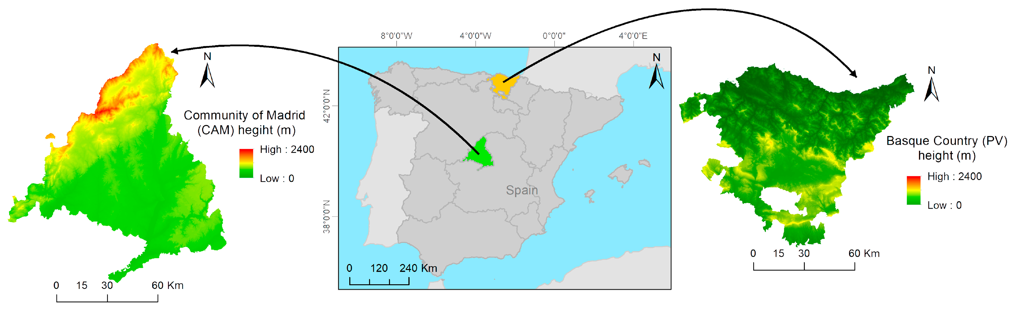
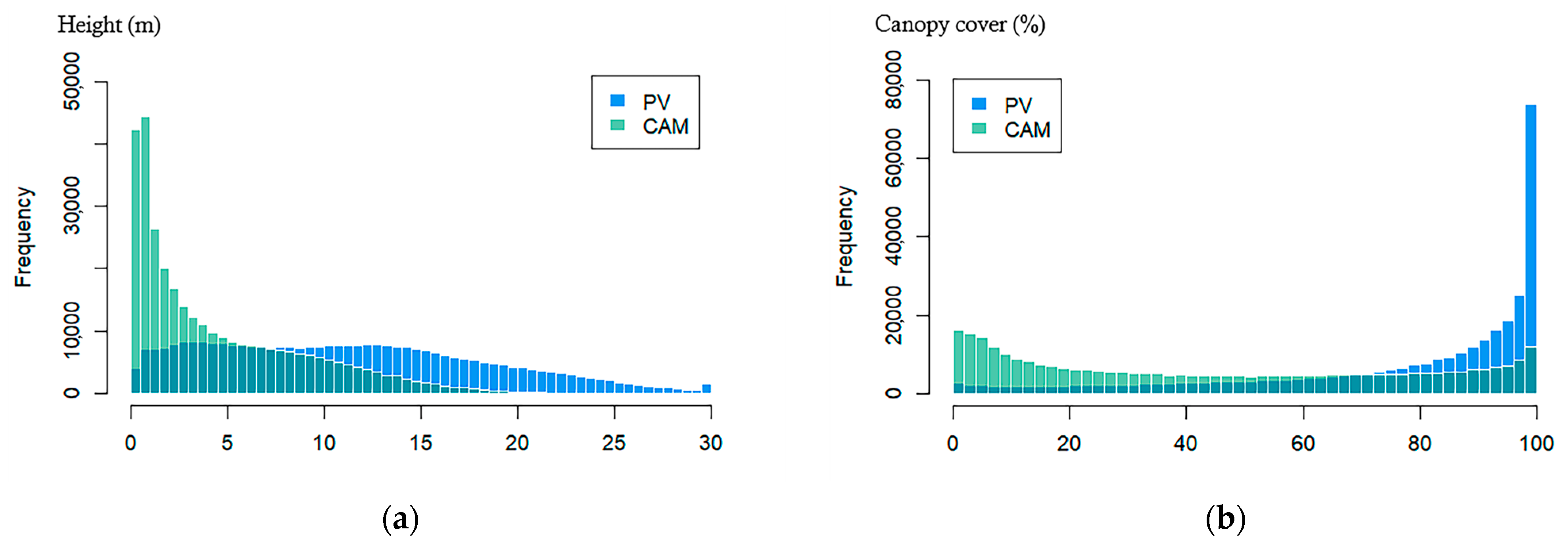
2.1. Study Area

The study was conducted in Spain, a southwestern European country (Figure 1), across two regions representative of temperate and Mediterranean forests. In the Iberian Peninsula, forest vegetation is shaped by climate, its interaction with topography, and the proximity to the sea [33]. The northern and north-western parts of the Iberian Peninsula experience a temperate climate characterized by mild winters and cool summers. These areas receive abundant rainfall throughout the year, supporting lush vegetation and dense forests. The central and southern regions have a Mediterranean climate characterized by hot and dry summers and mild and wet winters [34].

Our first study area is located in the Basque Country (PV, from Spanish “País Vasco”), in the northern part of the Iberian Peninsula (Figure 1). PV covers an area of 7234 Km², out of which 56% is forested [35]. The average monthly temperature ranges between 20 °C in summer and 5 °C in winter, with average annual precipitation ranging from 450 to 1000 mm, according to the Spanish Meteorological Agency (AEMET). The region is predominantly mountainous, with abrupt slopes and elevations that reach up to 2600 m above sea level. Forests are dominated by conifer species (Pinus radiata being the most common) and deciduous species, including oaks (Quercus pyrenaica, Q. robur, Q. petrea, Q. ilex), beech (Fagus sylvatica), and Eucalyptus plantations. Additionally, mixed forests occur where both deciduous and conifer species coexist, resulting in a unique blend of vegetation [36].

The second study area is located in the Madrid region (CAM, from Spanish “Comunidad Autónoma de Madrid”). CAM covers an area of 8028 Km² in the center of the country (Figure 1), out of which 24.34% is covered by trees, according to the National Forestry Inventory. With a central Mediterranean climate, the region is characterized by an average winter temperature of 1 °C and a summer temperature of 32 °C. The yearly average rainfall is 450 mm (AEMET). Sudden elevation changes characterize the landscape. Forests are primarily composed of evergreen species, including holm oaks (Quercus ilex), Pyrenean oak (Quercus pyrenaica), and pines (i.e., Pinus pinea, Pinus halepensis, Pinus pinaster) [37].

The forest vegetation in the selected areas is very different, both in terms of species composition and structure. Mediterranean forests (CAM) are more open (average FCC of 55%) with lower density and height (Figure 2), while the northern temperate forests (PV), managed for timber production, are denser (average FCC of 77%) and taller, with trees up to 30 m in height.

To estimate the forest structural variables of interest, we followed a standard workflow that includes image processing, statistical analysis, modelling, and validation (Figure 3). The reference data was obtained from the second national Spanish Lidar survey (2016–2017). FCC and CH were derived from the point cloud itself, whereas AGB was “spatialized” through modelling based on the fourth national forest inventory (NFI) in situ data. Random forest (RF) models were trained to estimate these forest variables from features derived from multispectral and SAR data. Different feature sets were assessed to select the most accurate combination for each study area and forest variable. Model temporal inference ability was analyzed using forest variables generated from the first (2010 CAM and 2012 PV) and third (2023 CAM) lidar flights. A detailed description of each step is provided in the following sections.

2.2. Remote Sensing Data

2.2.1. Lidar Data

Systematic lidar surveys are conducted by the Spanish National Geographic Institute (IGN) as part of the National Plan for Aerial Orthophotography (PNOA). Two comprehensive surveys are currently available, the first, covering the period 2008–2015, and the second, covering 2015–2021. The third lidar survey is currently available only for the Madrid region (2023). Data acquisition was performed using the footprint discrete return LEICA sensors ALS70 (PV) and ALS70HP (CAM) for the first and second flights. The point density was 0.5 points per square meter for the first flight (used for the independent validation) and 2 points per square meter for the second flight (used for model training). The third flight was performed using the ATLM Galaxy T2000 de Optech ALS80 sensor (CAM) with a point density of 5 points per square meter. Lidar data were processed using the Fusion Area Processor (AP) version 4.40, a software developed by the forestry branch of the United States Department of Agriculture (USDA) [38].

Lidar data were processed using the Fusion Area Processor (AP), a software developed by the forestry branch of the United States Department of Agriculture (USDA) [38]. Fusion was used to extract CH and FCC from the lidar measurements. Both variables required the estimation of the height above ground (i.e., normalized height). FCC was calculated as the proportion of first returns above a two-meter height from the total number of first returns reporting in the resolution cell. The canopy height was calculated as the 98th percentile of the height above ground. Aboveground biomass (AGB, Mg/ha) was modeled using a RF model trained with lidar-derived metrics (e.g., return proportion by 10 m strata, point density per strata, canopy average height, and standard deviation), and as reference, the in situ data from the 4th Spanish national forest inventory. AGB was calculated from the NFI’s tree measurements using species-specific allometric models [39]. A more in-depth description can be found in Tanase et al. [40].

2.2.2. Optical Imagery

The HLS product (NASA and USGS) was used as optical imagery. HLS contains harmonized surface reflectance images from the Operational Land Imager (OLI) sensor onboard the Landsat-8 satellite and the Multi-Spectral Instrument (MSI) sensors onboard Sentinel-2A/B satellites [21]. The HLS product is atmospherically corrected, spatially co-registered at 30 m resolution, and normalized as a nadir view. MSI bands are radiometrically adjusted to OLI spectral bands. Before the analysis, cloud, cloud shadow, and water bodies were masked using the quality assessment band provided with the data. For each image available in each year (n_CAM = 98 acquired in 2016; n_PV = 82 acquired in 2017), several indices were calculated, including the normalized vegetation index (NDVI, [41]), the normalized difference moisture index (NDMI, [42]), the normalized burn ratio (NBR, [43]), and the enhanced vegetation index (EVI, [44]). Furthermore, using the coefficients derived from Baig et al. [45], the Tasseled Cap (TC) transformations—Brightness, Wetness, and Greenness—proposed by Crist and Cicone [46] were computed. For all spectral bands and vegetation indices, annual percentiles (10, 25, 50, 75, and 90) were calculated using all images available in each year. The process was replicated for images acquired in 2023 for the CAM region (n_CAM = 235) to assess the temporal inference precision of the selected models.

Landsat 5 and 7 Collection 2 Level 2 imageries were used for past temporal inference, as no other optical source was available at the time of the first lidar flights (2010–CAM and 2012–PV), and these sensors are geometrically and radiometrically similar to the ones used in the HLS product. Landsat 5 imagery was incorporated to avoid the issues caused by the banding present on Landsat 7 imagery [47]. Band naming was harmonized across the sensors (TM, ETM+, OLI), and clouds, shadows, and water bodies were masked out using the quality assessment bands. Topographical effects were corrected as per Soenen et al. [48]. All vegetation indices and percentiles were calculated using the same methodology employed for the HLS data. The calculation of indices was conducted on a per-image basis. Utilizing the images from the entire year (n_CAM = 42; n_PV = 43), the same percentiles were computed (10, 25, 50, 75, and 90). It should be noted that the Landsat tiling system is different from the one used by the HLS. To ensure consistency, Landsat images were adjusted to the extent of the HLS tile used. Landsat 5 imagery was not available in Collection 2 Level 2 for PV and was therefore not used in the analysis.

2.2.3. Synthetic Aperture Radar Imagery

Single-look complex (SLC) images from two SAR missions, TerraSAR-X/TanDEM-X (TSX/TDX) and Sentinel-1 (S1), were used to derive radar metrics (i.e., backscatter and interferometric coherence) at X- and C-bands, respectively. Using the single-pass TSX/TDX acquisitions, the interferometric height was also computed.

All S1 images available for each reference year (CAM–2016 and PV–2017) were selected for the analysis (n_CAM = 69—relative orbits 001 and 081; n_PV = 69—relative orbits 081 and 103). S1 SLC images were multi-looked with a factor of 7 in range and 2 in azimuth to reduce speckle and bring the pixel size closer to the resolution intended for analysis (30 m). The first image of the series, by relative orbit, was used as the master with each successive acquisition being co-registered to the reference using an iterative procedure based on intensity matching and spectral diversity aided by the PNOA-Lidar digital elevation model [49]. Interferograms were produced from consecutive image pairs, with the DEM aiding in the simulation and subtraction of the topographic phase. Interferometric coherence was computed using a two-step adaptive approach for each interferogram. A lookup table (LUT) was created to orthorectify the SAR backscatter and coherence images using the master image and the DEM. The backscatter coefficient was calibrated to terrain-flattened γ⁰ [50], and a multi-temporal speckle filter was applied [51]. All SAR-derived metrics were resampled to 30 m to match the optical data grid, and the percentiles 10, 25, 50, 75, and 90 were computed for each S1 metric (co- and cross-polarized backscatter and coherence) by relative orbit.

TSX/TDX single-polarized (HH) imagery was used to provide information related to forest height through differential interferometric processing (DInSAR), which included the removal of the topographic phase based on the orbital information and a reference DEM. Interferometric processing was carried out using two acquisitions (one from each satellite) from the summers of 2018 in PV and 2019 for the CAM. To reduce phase noise, spatial averaging (i.e., multi-looking with a factor of 5 in both range and azimuth) was applied during interferogram generation. Furthermore, the interferograms were filtered with adaptive filtering based on the local fringe spectrum [52]. The DInSAR phase was unwrapped with the minimum cost flow algorithm and a coherence-based weighting factor [53]. To reduce phase noise, pixels with a coherence below 0.3 were masked out before unwrapping. The unwrapped phases were converted to elevation using the phase-to-height sensitivity. The relative heights were subsequently geocoded to the Universal Transverse Mercator (UTM) coordinate system at 10 m pixel spacing and debiased using as reference the lidar-derived canopy height (i.e., 99th percentile of normalized elevation). The geocoded heights were then adjusted to align the HLS resolution and extent.

2.2.4. Ancillary Data

The year of the most recent disturbance and its severity at pixel level (30 m spatial resolution) were used as ancillary information [54]. The disturbance database was obtained by combining dense Landsat time series from 1985 to 2023, spectral unmixing (i.e., which quantifies the fraction of different pure cover classes within a pixel) [55,56], and a change detection method (i.e., Continuous Change Detection and Classification) [47,57]. The algorithm was specifically calibrated to detect forest changes in temperate and Mediterranean forests in Spain [54]. Information on disturbances was included via two variables: the year of the last detected disturbance and its magnitude. The magnitude was calculated by determining the difference between the normalized difference fraction index (NDFI) after and before the perturbation. The NDFI was obtained using spectral unmixing and fractions of green vegetation (GV), non-photosynthetic vegetation (NPV), soil, shade, and cloud [55].

Elevation, slope, aspect, and roughness were derived from the national lidar-based DEM (available from IGN) and used as predictor variables, as they influence forest vegetation distribution [16,58]. The metrics were calculated as per Wilson et al. [59]. For the CAM, the forested area was masked using the Spanish Forest Map (MFE 1:25,000) available from the Ministry of the Environment, Territorial Planning and Sustainability repository. The repository is automatically updated with the 2022 version being used. For PV, forest maps were available on the PV geoportal (https://www.geo.euskadi.eus/, first accessed on 2 February 2022) for the years 2005, 2010, 2012, 2016, 2018, 2020, 2021, and 2022, with the 2018 map being selected as it is the closest to the lidar data used to generate the reference variables. For both regions, the main forest vegetation groups (e.g., pines, oaks, beach, mixed species) were extracted from the MFE and used as a qualitative (categorical) variable in the regression models.

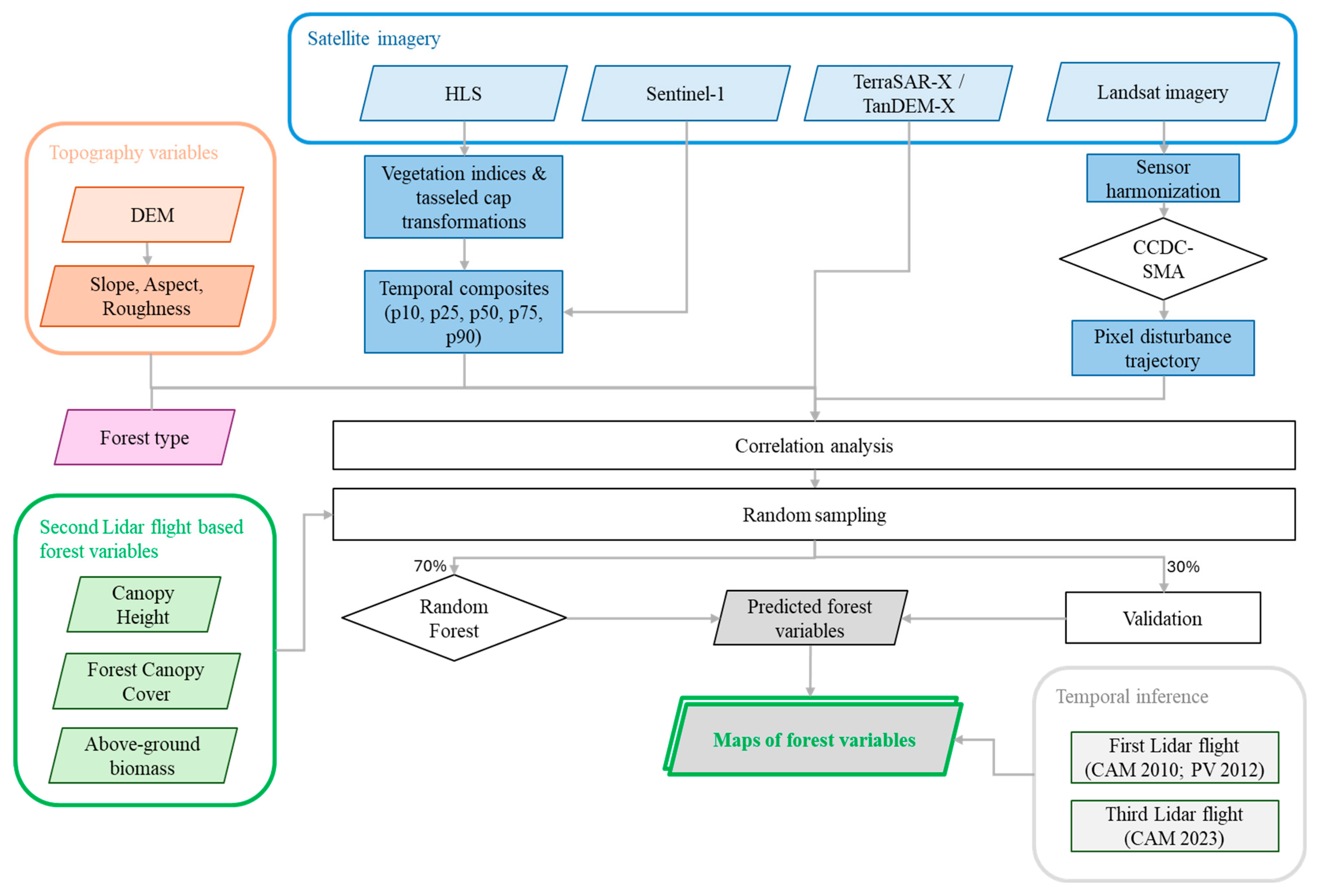
2.3. Modelling and Accuracy Assessment

2.3.1. Forest Variables Estimation

Random forest models [60] were fitted to predict forest variables for each site using different feature sets. This machine learning algorithm is frequently used to estimate forest biophysical parameters [18] as it is more flexible than parametric approaches, is robust to outliers, and can handle large datasets [15]. RF models were trained to estimate CH, FCC, and AGB using a fixed number of trees (ntree = 600).

Seven models, based on different sensor combinations (see below), were trained using 70% of the data and validated over the remaining 30% for each region (HLS tile T30TVL for the CAM and T30TWN for PV). Prior to the development of the RF models, an exploratory analysis was conducted to evaluate the correlation (using Spearman’s and Pearson’s) between the predictor variables. The analysis was performed on 50% of all forest pixels. Predictor variables with correlation values above 0.9 were excluded (i.e., the alphabetically first variable was kept). The evaluated models were:

• A model based on HLS optical data (benchmark).
• An extended optical model that incorporated information on disturbances.
• A model based on C-band Sentinel-1 variables (backscatter and coherence).
• A SAR-only model combining Sentinel-1 and TSX/TDX variables.
• A model combining HLS and Sentinel-1 variables.
• A model combining HLS, Sentinel-1, and information on disturbances.
• A ‘full’ model including all the explanatory variables.

Notice that all models incorporated topographic variables and the main forest species, if not correlated. To ensure consistency across forest types and time, all data were processed using a common methodology, and summary statistics (e.g., percentiles) were used to capture seasonal variability. Except for TSX/TDX, all datasets are freely accessible, thereby facilitating reproducibility.

2.3.2. Model Evaluation and Performance

The independent validation data was used to calculate the coefficient of determination (R²) between observed and predicted values, the root mean squared error (RMSE, Equation (1)), and the mean absolute error (MAE, Equation (2)) for each model combination, variable, and region.

$$RMSE=\sqrt{{\displaystyle \frac{{\sum }_{i=1}^n{({Predicted}_i-{Observed}_i)}^2}{n}}}$$

(1)

where n is the total number of observations used in the comparison between predicted and observed values.

$$MAE={\displaystyle \frac{1}{n}}{\sum }_{i=1}^n\left|{Predicted}_i-{Observed}_i\right|$$

(2)

where n is the total number of prediction-observation pairs used in the calculation.

The most efficient model, in terms of R², RMSE, and MAE, was evaluated across time, i.e., temporal inference. For the CAM, further temporal inference was performed for CH and FCC using the third lidar flight data as reference. AGB model evaluation was not possible due to the lack of contemporaneous in situ NFI data. Temporal inference was also performed using the data acquired by the first lidar flight as a reference. This analysis was constrained by the availability of Sentinel-2, Sentinel-1, and TSX/TDX acquisitions. Given these constraints, the optical models were utilized by taking advantage of the Landsat 5 and 7 images acquired in the same years as the first lidar flights (CAM in 2010; PV in 2012).

3. Results

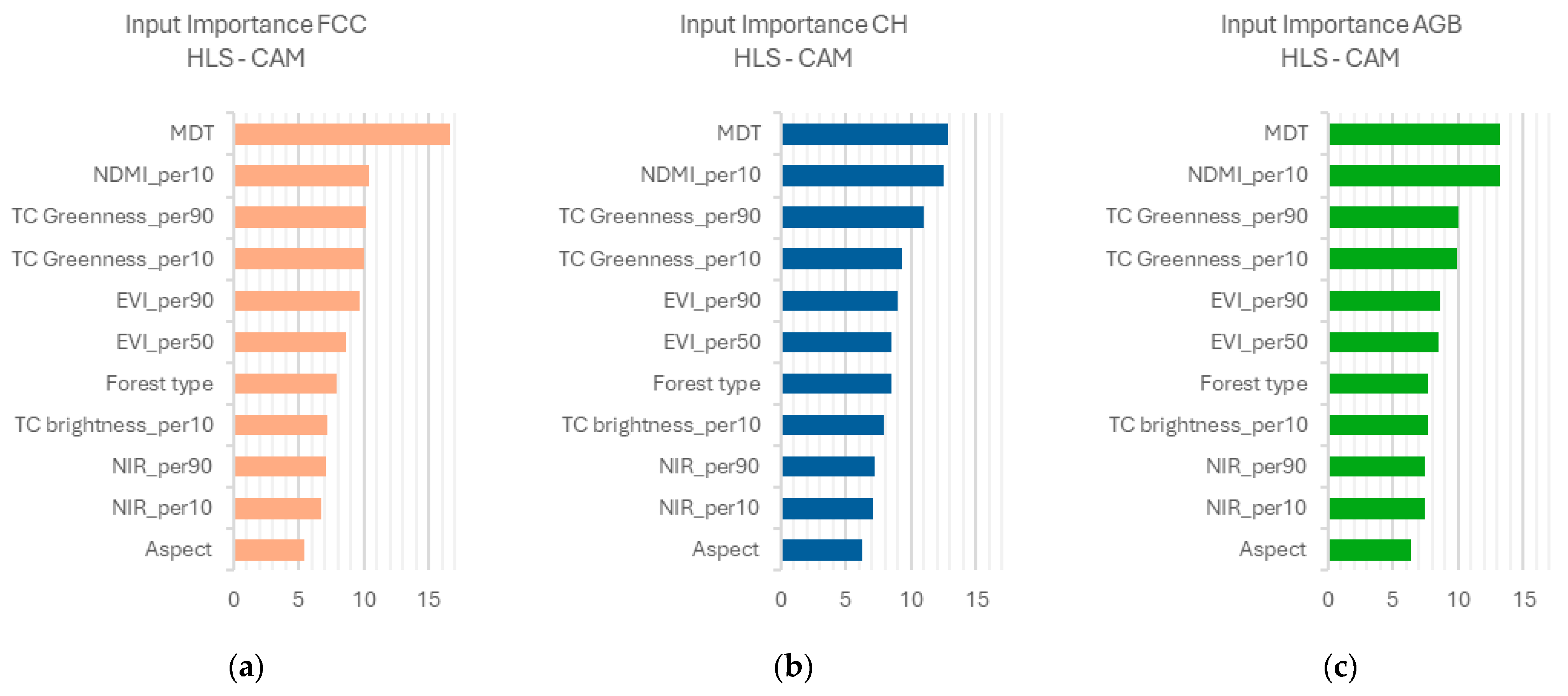
3.1. Mediterranean Forests

For FCC, the model integrating all predictors (

Table 1. Modelling errors for different sensor combinations in the region of the Basque Country (PV) 2017 and the region of Madrid (CAM) 2016.

Model	Forest Variable	CAM			PV
		R2	RMSE	MAE	R2	RMSE	MAE
Optical-based models
HLS	FCC	0.77	14.47	11.08	0.58	17.28	13.30
	CH	0.81	1.76	1.19	0.56	4.49	3.51
	AGB	0.77	29.44	21.58	0.49	115.60	88.97
HLS and disturbance data	FCC	0.74	13.54	10.38	0.60	17.93	14.28
	CH	0.68	2.05	1.56	0.53	3.74	2.88
	AGB	0.63	34.41	27.13	0.43	95.94	70.85
Radar-based models
Sentinel-1	FCC	0.40	23.44	19.17	0.45	19.52	15.07
	CH	0.47	2.94	2.10	0.51	4.72	3.64
	AGB	0.47	44.33	33.76	0.46	118.97	89.95
Sentinel-1 and TSX/TDX	FCC	0.67	17.33	13.56	0.46	16.69	12.63
	CH	0.80	1.79	1.22	0.68	3.65	2.72
	AGB	0.78	28.33	20.74	0.65	92.64	67.08
Mixed models
HLS and Sentinel-1	FCC	0.77	14.55	11.15	0.61	16.70	12.79
	CH	0.81	1.76	1.20	0.64	4.10	3.16
	AGB	0.77	29.26	21.49	0.58	105.76	80.09
HLS, Sentinel-1, and disturbance data	FCC	0.75	13.29	10.19	0.63	17.27	13.69
	CH	0.70	2.01	1.52	0.59	3.52	2.69
	AGB	0.65	33.68	26.57	0.50	99.75	76.22
HLS, Sentinel-1, disturbance data, and TSX/TDX	FCC	0.76	12.90	9.90	0.61	16.31	12.94
	CH	0.79	1.67	1.23	0.68	3.00	2.24
	AGB	0.75	28.47	21.75	0.62	75.86	53.87

All models include, if non-correlated forest type and the topography-related predictor variables.

) achieved the lowest errors (RMSE = 12.90% and MAE = 9.90%), although models using only HLS data had a marginally higher R² (0.77). For CH, the HLS-based model was the most accurate, with an MAE of 1.19 m and an R² of 0.81. Adding Sentinel-1 data to HLS did not meaningfully enhance performance for CH, with accuracy metrics remaining nearly unchanged. In contrast, models based solely on Sentinel-1 data yielded the weakest performance across both variables. For example, the CH model had the lowest R² (0.47) when only using Sentinel-1. However, incorporating structural data from TSX/TDX alongside Sentinel-1 markedly improved CH estimates, with RMSE (1.79 m) and MAE (1.22 m) nearly matching the accuracy of HLS-based models. For AGB, the HLS-only model and the combined HLS and Sentinel-1 model yield results that are highly analogous. A similar phenomenon is observed for those same models for the FCC and CH, as the error values are nearly identical. Combining Sentinel-1 and TSX/TDX data leads to the highest R² for AGB estimation (R² = 0.78), along with the lowest RMSE (28.33 Mg/ha) and MAE (20.74 Mg/ha).

Models that incorporate disturbance information tend to show lower R² values. Specifically, precision decreases by approximately 16% when disturbance data is added to the HLS and Sentinel-1 model (AGB from R² = 0.77 to 0.65), and by around 18% when added to the HLS-only model (AGB from R² = 0.77 to 0.63). In the case of AGB, the lowest-performing model remains the one based on Sentinel-1, with the lowest R² (0.47) and the highest errors (RMSE = 44.33 Mg/ha, MAE = 33.76 Mg/ha). Overall, the most accurate models (highest R² and lowest RMSE and MAE), excluding those based on temporally sparse TSX/TDX data, were derived from HLS imagery. These models were therefore selected for temporal inference.

Analyzing the HLS model predictor variables shows a consistent ranking according to RF importance. The elevation (MDT) stands out as the most crucial predictor (Figure 4) with an importance score (i.e., the decrease in mean squared error when including the variable across all model nodes) of over 12% in all cases.

Variables such as the 10th NDMI percentile (exceeding 10% in all cases) and the Tasseled Cap Greenness 90th percentile (~10% or higher) consistently show high importance values (i.e., relevant information content), ranking among the most influential across all models. Predictor variables, such as the EVI 50th percentile, forest type, and NIR 10th percentile, remain consistently present across models, although their relative influence varies depending on the specific model.

3.2. Temperate Forests

In the PV region, integrating different sensor types generally improves estimation accuracy (Table 1). Forest canopy cover was best estimated using models that included optical imagery and disturbance history, while radar-only models performed the worst, with R² values below 0.5. Adding TSX/TDX data to the HLS and Sentinel-1 data did not improve FCC prediction, while a combination of S1 and TSX/TDX data yielded low R² values (0.46). Overall, accuracy differences across FCC models were relatively small, except for the notable underperformance of radar-based models.

For CH, models that incorporated TSX/TDX structural information—specifically the combinations of Sentinel-1 and TSX/TDX model, and HLS, S1, disturbance data, and TSX/TDX model—achieved the highest R² values (both 0.68) and the lowest estimation errors (RMSE = 3.00 m, MAE = 2.24 m for the HLS, S1, disturbance, and TSX/TDX model). In contrast, models based on Sentinel-1 data produced the least accurate estimates (MAE = 3.64 m, RMSE = 4.72 m for CH). Among models excluding TSX/TDX data, the HLS and S1 combination was the most accurate for CH (RMSE = 4.10 m, MAE = 3.16 m).

Similarly, for AGB, models incorporating TSX/TDX data achieved the highest R² values, although error metrics varied depending on the data combination. Sentinel-1 alone was the least effective (RMSE = 118.97 Mg/ha, MAE = 89.95 Mg/ha, and R² = 0.46 for AGB), but its performance improved when combined with other data sources (R² = [0.50–0.65]). Optical-only models also underperformed, with R² below 0.50 for AGB. Adding disturbance data reduced AGB estimation errors (RMSE = 99.75 Mg/ha, MAE = 76.22 Mg/ha) while the R² of the HLS and S1 model was noticeably higher (0.58 vs. 0.50).

According to these results, the HLS and Sentinel-1 models offer the best trade-off between accuracy (high R² > 0.58, low RMSE, and MAE) for the set of variables analyzed, computational efficiency, and independence from the limited availability of TSX/TDX data. The number of uncorrelated predictors used for modelling was 27 (Figure 5). The importance of the Sentinel-1 parameters is particularly notable, especially the S1 interferometric coherence (S1_xx_coh) being ranked as the most significant variable for estimating CH and AGB. These models show considerable similarity in ranking the importance of predictor variables, with the main difference being that the VH component of the S1 backscatter (S1 vh_per10) was more relevant when estimating CH, while the VV component (S1 vv_per10) was more relevant for AGB.

The 90th percentile of the Tasseled Cap Brightness (TC Brightness_per90) is the second most important variable for both CH and AGB (over 6%), and the third for FCC, while, unlike CAM, elevation (MDT) importance ranks lower (<5%) for AGB and CH. Conversely, for FCC, the importance of the elevation (MDT, ~10%) is higher, followed by the S1-derived variables.

3.3. Temporal Inference: HLS Models

When applying the calibrated HLS models to extrapolate forest structural variables over time, a decrease in the explanatory power is observed for the Mediterranean forests in 2010 and 2023 compared to the year of model calibration (2016), as evidenced by reductions in R² values for both FCC and CH (

Table 2. Results for temporal inference using HLS models calibrated in 2016 and applied to Landsat (2010) and HLS (2023) data over Mediterranean forests (CAM).

Region of Madrid (2010)
Forest Variable	R2	RMSE	MAE
FCC	0.51	27.86	22.90
CH	0.57	2.58	2.15
AGB	0.59	45.28	36.59
Region of Madrid (2023)
Forest Variable	R2	RMSE	MAE
FCC	0.61	19.67	15.55
CH	0.55	5.41	4.04

). For FCC, the R² decreased from 0.77 in 2016 to 0.51 in 2010 and 0.61 in 2023. However, a notable reduction in error is observed between 2010 and 2023, with RMSE decreasing from 27.86% to 19.67%, and MAE from 22.90% to 15.55%. The 2023 RMSE is closer to the model performance in 2016 (RMSE = 14.47%). For CH, the decline in R² is also evident, dropping from 0.81 in 2016 to 0.57 in 2010 and 0.55 in 2023. RMSE increased from 1.76 m (2016) to 2.58 m (2010), and further to 5.41 m in 2023, with a corresponding MAE of 2.15 m and 4.04 m, respectively. AGB shows similar patterns, with RMSE increasing from 29.44 Mg/ha in 2016 to 45.28 Mg/ha in 2010. The lack of reference field data precluded validation of the AGB model in 2023.

The temporal inference results indicated suboptimal performance of the models in terms of R², RMSE, and MAE for the temperate forests (

Table 3. Results for temporal inference using HLS models calibrated in 2017 and applied to Landsat (2012) data over temperate forests (PV).

Region of the Basque Country (2012)
Forest Variable	R2	RMSE	MAE
FCC	0.13	32.99	28.97
CH	0.03	8.62	7.85
AGB	0.03	217.88	205.52

). Specifically, the models grounded in optical and disturbance data exhibited notable inaccuracies, particularly regarding CH and AGB. The models yielded an R² of 0.13 for forest canopy cover (FCC), while for CH and AGB, the R² was 0.03.

4. Discussion

In this study, we develop a workflow to estimate key forest biophysical variables (i.e., forest canopy cover, canopy height, and aboveground biomass) across two representative regions in peninsular Spain. To capture structural detail and spatial-temporal variations, we explored multiple combinations of remote sensing data sources, integrating information from lidar, optical, and radar sensors, as well as past disturbance history. Each data source contributed unique strengths: lidar provided precise vertical forest structure for model training and validation; HLS offered frequent observations and a broad spatial coverage; Sentinel-1 and TSX/TDX contributed cloud-independent structural-related information, while disturbance data helped contextualize canopy changes.

4.1. Mediterranean Forests

Over Mediterranean forests, characterized by an open structure and low vegetation heights in a predominantly cloud-free environment, models based on predictor variables derived from optical imagery achieved higher R² and lower RMSE when compared to models incorporating additional predictor variables derived from radar data. Saturation of the C-band at relatively low biomass levels [61] and an open forest structure, with the associated increase in signal from the soil, may have influenced the relevance of such data when characterizing forest structure. These results align with existing literature [62], as the influence of soil water content weakens the relationship between radar backscatter and AGB. Nevertheless, other studies suggest that a combination of L- and C-band SAR (ALOS2 and Sentinel-1) with optical data (Landsat 8) is effective for estimating AGB of pine plantations in southeastern Spain, with R² values ranging from 0.60 to 0.68 [63]. Our findings (AGB HLS and S1 model, R² = 0.77) demonstrate improved performance. This improvement can be attributed, at least in part, to the integration of HLS imagery, which substantially augmented the temporal frequency of the images by combining Landsat and Sentinel-2 data. The model that utilizes solely optical data (HLS) also yields similar outcomes, thereby highlighting the importance of using multiple optical data sources.

The findings accentuate the elevation role as the most influential variable in all models when predicting forest structure, with vegetation indices (i.e., NDMI, Tasseled Cap Brightness, EVI) playing a secondary role. This suggests that topography (e.g., elevation) significantly influences the distribution and growth of forest species in the Mediterranean region, in agreement with previous studies that found a robust relationship between topography and forest dynamics [16,58]. Interferometric heights derived from TSX/TDX did not enhance the accuracy of the estimates. This is primarily because low heights and open canopy structures render such information less relevant. Specifically, the measured scattering center becomes an average value of vegetation and soil surface, which is modulated by the distance between trees rather than their height. For FCC in the Mediterranean, including radar data did not improve estimations over using optical data alone, as also observed by other studies [64]. Only marginal improvements were observed for AGB when adding the Sentinel-1- or TSX/TDX-derived variables. The increased importance of TC Brightness for the estimation of forest variables in the Mediterranean forests might be related to the increased soil exposed, while TC Greenness increased importance may be linked to the density of vegetation cover, particularly over the northern forests [65].

In agreement with other studies [66], information on disturbances appears to be less relevant when events are rare or affect small areas, such as in the CAM region, where non-stand-replacing disturbances (such as drought-induced dieback and defoliation) are more common but harder to detect [54]. In this region, water is also a limiting factor, thereby influencing the recovery process after a disturbance occurs [67]. Mediterranean vegetation is adapted to drought conditions, which implies a limited phenological response to disturbances (e.g., they do not generate evident or immediate regrowth) as water availability is the primary factor determining growth rather than sporadic disturbances [68]. This reduces the spectral variability detectable by optical sensors, making it challenging to identify significant changes in vegetation.

4.2. Temperate Forests

In contrast to the Mediterranean region, the interferometric height derived from X-band data proved to be a significant predictor for characterizing CH and AGB in the taller and denser temperate forests. The use of Sentinel-1 data yielded low estimation results (R² < 0.51), consistent with the findings of previous studies [69]. The integration of optical and radar data into a unified model has been demonstrated to provide a substantial benefit for the estimation of temperate forest variables compared with models that rely on solitary data sources [69,70]. Combining X- and C- band data may compensate for the lack of optical data in environments with frequent cloud cover when estimating forest structural attributes [69], such as AGB and CH, particularly compared to Sentinel-1 alone (S1 and TSX/TDX model R² = 0.65 vs. S1 model R² = 0.46 for AGB in PV). Combining HLS and Sentinel-1 data provided improvements of 9%–10% in RMSE for both CH and AGB when compared to HLS-only models. Specifically, the RMSE dropped from 4.49 m to 4.10 m for CH, while for AGB it dropped from 115.60 to 105.76 Mg/ha. Further improvements were observed when using a model that integrates all datasets: HLS, S1, disturbance history, and TSX/TDX. This setup reduces the RMSE by approximately 33% (to 3.00 m) for CH and by about 34% (to 75.86 Mg/ha) for AGB compared to the HLS-only model. Across all forest variables, Sentinel-1-based models yield higher RMSE and lower R² values, indicating lower predictive performance. Over the temperate forests, the TC Wetness provided important information for FCC estimation, as also observed in previous studies [66,71]. This suggests that TC Wetness and NDMI are important variables when estimating forest attributes across a wide range of environments. Over the temperate region (i.e., PV), logging is a common practice (usually Pinus radiata and Eucalyptus species), resulting in disturbance information playing a greater role when modelling forest structural variables. In areas with intensive forest management practices, the presence of abrupt disturbance is more frequent [54] as forest areas undergo repeated management interventions.

4.3. Temporal Inference

In the Mediterranean forests, the calibrated HLS models demonstrated a decline in explanatory power over time, as evidenced by decreasing R² values for FCC and CH when applied to data from 2010 and 2023, compared to the calibration year (2016). This trend suggests a reduced ability to generalize beyond the model calibration year [72]. Despite this decline, model accuracy for FCC improved in more recent years: the RMSE decreased from 27.86% in 2010 to 19.67% in 2023, approaching the value (14.47%) obtained for 2016 (year of model training). These improvements may reflect the difference in the satellite imagery used (only Landsat against the combination of Landsat and Sentinel-2 of the HLS product). In contrast, the performance for CH was less consistent. The R² for CH showed a decline (from 0.81 in 2016 to 0.55 in 2023), while RMSE increased significantly, especially in 2023, where it reached 5.41 m. However, such differences may have been exacerbated by external factors related to the ALS sensors used to acquire the reference data. The mean difference between the average forest height (CAM region) estimated from the second (2016) and the third (2023) lidar flight (4.64 m) is partially explained by the use of different elevation models for height normalization (0.30 m) and partially by the annual forest’s growth (0.08 m/year according to the 3rd and 4th FNI data). However, the remainder (3.78 m) seems to be entirely related to the increased point cloud density for the third flight, as a greater number of points per square meter increases the likelihood of capturing the canopy’s highest and lowest features. As models are calibrated with less precise data (i.e., 2016 Lidar-derived height), the increment in RMSE was somewhat expected. For the temperate forests, temporal inference yielded substantially lower model performance across all variables. R² values for FCC, CH, and AGB were 0.13, 0.03, and 0.03, respectively. These results may be related to limited image availability in 2012 (Landsat 5 not available in the Collection 2 Level 2), scan line corrector failure in Landsat 7 imagery [73], and high cloud cover, which translates into a loss of information for the predictor variables (percentiles) computed from annual data.Haga clic o pulse aquí para escribir texto.

4.4. Limitations

The results underscore an important methodological limitation: the temporal transferability of models, which is limited by changes in sensor characteristics, reference data quality, and region-specific factors. Further, as optical sensors are sensitive to forest cover [74,75], errors in the forest type layer can propagate into biomass and structure estimates [76], especially in regions dominated by fast-growing species such as Eucalyptus [69], as occurs in PV. A further constraint in dense and mature forests is the saturation of satellite signals, particularly relevant for optical and shorter-wavelength radar data, which diminishes sensitivity to forest structure and leads to underestimation of aboveground biomass [77]. In the northern temperate region, the quality of available Landsat imagery (Landsat 7 SLC-off) and the absence of Landsat 5 data in Collection 2 Level 2 for the required period likely influenced the performance of the optical-based models, as the region is frequently affected by cloud cover.

From a methodological perspective, while random forest regression has proven to be a robust technique in the field of remote sensing, it is not without its inherent limitations. The efficacy of the algorithm depends on the characteristics of the data and its tendency to struggle with extrapolation and interpretability [78]. The lack of TSX/TDX data prevented the most accurate models from being used for temporal inference. While TSX/TDX data improved predictions in PV, their limited spatial and temporal coverage and restricted accessibility pose challenges for routine, large-scale, or temporal applications. These constraints hamper their operational deployment despite the observed performance benefits.

5. Conclusions

This study highlights the trade-offs when using diverse data sources for estimating key forest biophysical variables across different biomes. Our findings reveal the strengths and limitations of combining lidar, HLS, Sentinel-1, and TSX/TDX along with disturbance data to improve forest variable estimation across time and environmental conditions.

The results for the Mediterranean forests highlight that models based primarily on optical imagery performed better, as evidenced by higher R² values for FCC and CH. Temporal extrapolation of the models to years outside the calibration period showed a decline in model performance, particularly for FCC and CH. However, forest growth and increased point densities for the latest lidar sensors partially accounted for these discrepancies. Substantially lower model performance was observed across all variables in the temperate forests. Disturbances (e.g., logging and wildfires) played a significant role in altering forest structure, which in turn improved model predictions in these forests.

Overall, this study demonstrates that integrating multiple remote sensing datasets, including lidar, optical, and SAR imagery, can improve the estimation of forest biophysical variables in certain areas. However, the challenges highlighted in this research, particularly in terms of temporal extrapolation and sensor-specific limitations, suggest the need for further refinement in model calibration. Nevertheless, these insights contribute to a more nuanced understanding of forest structure estimation and highlight areas for future research.

References

1. Pan, Y.; Birdsey, R.A.; Phillips, O.L.; Houghton, R.A.; Fang, J.; Kauppi, P.E.; Keith, H.; Kurz, W.A.; Ito, A.; Lewis, S.L.; et al. The enduring world forest carbon sink. Nature 2024, 631, 563–569. [Google Scholar] [CrossRef] [PubMed]
2. Keenan, R.J. Climate change impacts and adaptation in forest management: A review. Ann. For. Sci. 2015, 72, 145–167. [Google Scholar] [CrossRef]
3. Senf, C.; Pflugmacher, D.; Hostert, P.; Seidl, R. Using Landsat time series for characterizing forest disturbance dynamics in the coupled human and natural systems of Central Europe. ISPRS J. Photogramm. Remote Sens. 2017, 130, 453–463. [Google Scholar] [CrossRef]
4. Van Lierop, P.; Lindquist, E.; Sathyapala, S.; Franceschini, G. Global forest area disturbance from fire, insect pests, diseases and severe weather events. For. Ecol. Manag. 2015, 352, 78–88. [Google Scholar] [CrossRef]
5. San-Miguel-Ayanz, J.; Durrant, T.; Boca, R.; Maianti, P.; Libertà, G.; Oom, D.; Branco, A.; De Rigo, D.; Ferrari, D.; Roglia, E.; et al. Advance Report on Forest Fires in Europe, Middle East and North Africa; Publications Office of the European Union: Luxembourg, 2023. [Google Scholar]
6. FOREST EUROPE; FAO; UNECE. State of Forests and Sustainable Forest Management in Europe 2020; Forest Europe: Zvolen, Slovak Republic, 2020. [Google Scholar]
7. Chuvieco, E. Teledetección Ambiental: La Observación de la Tierra Desde el Espacio; Editorial Ariel: Barcelona, Spain, 2010; ISBN 9788434434981. [Google Scholar]
8. Ahmed, O.S.; Franklin, S.E.; Wulder, M.A.; White, J.C. Characterizing stand-level forest canopy cover and height using Landsat time series, samples of airborne LiDAR, and the Random Forest algorithm. ISPRS J. Photogramm. Remote Sens. 2015, 101, 89–101. [Google Scholar] [CrossRef]
9. Huang, R.; Zhu, J. Using Random Forest to integrate lidar data and hyperspectral imagery for land cover classification. In Proceedings of the 2013 IEEE International Geoscience and Remote Sensing Symposium—IGARSS, Melbourne, VIC, Australia, 21–26 July 2013; pp. 3978–3981. [Google Scholar] [CrossRef]
10. Koetz, B.; Morsdorf, F.; Sun, G.; Ranson, K.J.; Itten, K.; Allgöwer, B. Inversion of a lidar waveform model for forest biophysical parameter estimation. IEEE Geosci. Remote Sens. Lett. 2006, 3, 49–53. [Google Scholar] [CrossRef]
11. Hu, X.; Shi, L.; Lin, G.; Lin, L. Comparison of physical-based, data-driven and hybrid modeling approaches for evapotranspiration estimation. J. Hydrol. 2021, 601, 126592. [Google Scholar] [CrossRef]
12. Nguyen, T.H.; Jones, S.; Soto-Berelov, M.; Haywood, A.; Hislop, S. Landsat Time-Series for Estimating Forest Aboveground Biomass and Its Dynamics across Space and Time: A Review. Remote Sens. 2020, 12, 98. [Google Scholar] [CrossRef]
13. García, M.; Riaño, D.; Chuvieco, E.; Danson, F.M. Estimating biomass carbon stocks for a Mediterranean forest in central Spain using LiDAR height and intensity data. Remote Sens. Environ. 2010, 114, 816–830. [Google Scholar] [CrossRef]
14. Senf, C.; Mori, A.S.; Müller, J.; Seidl, R. The response of canopy height diversity to natural disturbances in two temperate forest landscapes. Landsc. Ecol. 2020, 35, 2101–2112. [Google Scholar] [CrossRef]
15. Pourshamsi, M.; Xia, J.; Yokoya, N.; Garcia, M.; Lavalle, M.; Pottier, E.; Balzter, H. Tropical forest canopy height estimation from combined polarimetric SAR and LiDAR using machine-learning. ISPRS J. Photogramm. Remote Sens. 2021, 172, 79–94. [Google Scholar] [CrossRef]
16. Viana-Soto, A.; García, M.; Aguado, I.; Salas, J. Assessing post-fire forest structure recovery by combining LiDAR data and Landsat time series in Mediterranean pine forests. Int. J. Appl. Earth Obs. Geoinf. 2022, 108, 102761. [Google Scholar] [CrossRef]
17. Yu, Y.; Li, M.; Fu, Y. Forest type identification by random forest classification combined with SPOT and multitemporal SAR data. J. For. Res. 2018, 29, 1407–1414. [Google Scholar] [CrossRef]
18. Coops, N.C.; Tompalski, P.; Goodbody, T.R.H.; Queinnec, M.; Luther, J.E.; Bolton, D.K.; White, J.C.; Wulder, M.A.; Van Lier, O.R.; Hermosilla, T. Modelling lidar-derived estimates of forest attributes over space and time: A review of approaches and future trends. Remote Sens. Environ. 2021, 260, 112477. [Google Scholar] [CrossRef]
19. Woodcock, C.E.; Allen, R.; Anderson, M.; Belward, A.; Bindschadler, R.; Cohen, W.; Gao, F.; Goward, S.N.; Helder, D.; Helmer, E.; et al. Free access to Landsat imagery. Science 2008, 320, 1011. [Google Scholar] [CrossRef]
20. Hansen, M.C.; Loveland, T.R. A review of large area monitoring of land cover change using Landsat data. Remote Sens. Environ. 2012, 122, 66–74. [Google Scholar] [CrossRef]
21. Claverie, M.; Ju, J.; Masek, J.G.; Dungan, J.L.; Vermote, E.F.; Roger, J.C.; Skakun, S.V.; Justice, C. The harmonized Landsat and Sentinel-2 surface reflectance data set. Remote Sens. Environ. 2018, 219, 145–161. [Google Scholar] [CrossRef]
22. Herold, M.; Skutsch, M. Monitoring, Reporting and Verification for National REDD+ Programmes: Two Proposals. Environ. Res. Lett. 2011, 6, 014002. [Google Scholar] [CrossRef]
23. Liao, Z.; Liu, X.; van Dijk, A.; Yue, C.; He, B. Continuous Woody Vegetation Biomass Estimation Based on Temporal Modeling of Landsat Data. Int. J. Appl. Earth Obs. Geoinf. 2022, 110, 102811. [Google Scholar] [CrossRef]
24. Tanase, M.A.; Villard, L.; Pitar, D.; Apostol, B.; Petrila, M.; Chivulescu, S.; Leca, S.; Borlaf-Mena, I.; Pascu, I.S.; Dobre, A.C.; et al. Synthetic Aperture Radar Sensitivity to Forest Changes: A Simulations-Based Study for the Romanian Forests. Sci. Total Environ. 2019, 689, 1104–1114. [Google Scholar] [CrossRef]
25. Hajnsek, I.; Busche, T.; Abdullahi, S.; Bachmann, M.; Baumgartner, S.V.; Bojarski, A.; Bueso-Bello, J.L.; Esch, T.; Fritz, T.; Alonso-Gonzalez, A.; et al. TanDEM-X: The 4D Mission Phase for Earth Surface Dynamics: Science Activities Highlights and New Data Products after 15 Years of Bistatic Operations. IEEE Geosci. Remote Sens. Mag. 2025. [Google Scholar] [CrossRef]
26. Gomez, C.; Lopez-Sanchez, J.M.; Romero-Puig, N.; Zhu, J.; Fu, H.; He, W.; Xie, Y.; Xie, Q. Canopy Height Estimation in Mediterranean Forests of Spain with TanDEM-X Data. IEEE J. Sel. Top. Appl. Earth Obs. Remote Sens. 2021, 14, 2956–2970. [Google Scholar] [CrossRef]
27. Trier, Ø.D.; Salberg, A.B.; Haarpaintner, J.; Aarsten, D.; Gobakken, T.; Næsset, E. Multi-Sensor Forest Vegetation Height Mapping Methods for Tanzania. Eur. J. Remote Sens. 2018, 51, 587–606. [Google Scholar] [CrossRef]
28. Wang, J.; Xiao, X.; Bajgain, R.; Starks, P.; Steiner, J.; Doughty, R.B.; Chang, Q. Estimating Leaf Area Index and Aboveground Biomass of Grazing Pastures Using Sentinel-1, Sentinel-2 and Landsat Images. ISPRS J. Photogramm. Remote Sens. 2019, 154, 189–201. [Google Scholar] [CrossRef]
29. Liao, Z.; Van Dijk, A.I.J.M.; He, B.; Larraondo, P.R.; Scarth, P.F. Woody Vegetation Cover, Height and Biomass at 25-m Resolution across Australia Derived from Multiple Site, Airborne and Satellite Observations. Int. J. Appl. Earth Obs. Geoinf. 2020, 88, 102066. [Google Scholar] [CrossRef]
30. Tanase, M.A.; Nova, J.P.G.; Marino, E.; Aponte, C.; Tomé, J.L.; Yáñez, L.; Madrigal, J.; Guijarro, M.; Hernando, C. Characterizing Live Fuel Moisture Content from Active and Passive Sensors in a Mediterranean Environment. Forests 2022, 13, 1846. [Google Scholar] [CrossRef]
31. Næsset, E. Area-Based Inventory in Norway—From Innovation to an Operational Reality. In Forestry Applications of Airborne Laser Scanning; Maltamo, M., Næsset, E., Vauhkonen, J., Eds.; Springer: Dordrecht, The Netherlands, 2014; Volume 27. [Google Scholar] [CrossRef]
32. Magnussen, S.; Nord-Larsen, T.; Riis-Nielsen, T. Lidar supported estimators of wood volume and aboveground biomass from the Danish national forest inventory (2012–2016). Remote Sens. Environ. 2018, 211, 146–153. [Google Scholar] [CrossRef]
33. Rivas Martínez, S.; Gandullo, J.M. Memoria del Mapa de Series de Vegetación de España: 1:400.000; ICONA: Madrid, Spain, 1987. [Google Scholar]
34. Agencia Estatal de Meteorología (AEMET); Instituto de Meteorologia de Portugal. Atlas Climático Ibérico/Iberian Climate Atlas; AEMET: Madrid, Spain, 2011. [Google Scholar]
35. HAZI Fundazioa. El Bosque Vasco en Cifras 2022; HAZI: Vitoria-Gasteiz, Spain, 2022. [Google Scholar]
36. Gurrutxaga San Vicente, M. Patrones de Cobertura y Protección de los Bosques en el País Vasco. Geographicalia 2008, 53, 49–72. [Google Scholar] [CrossRef]
37. Comunidad de Madrid. El Medio Ambiente de la Comunidad de Madrid 2006–2007; Comunidad de Madrid: Madrid, Spain, 2007. [Google Scholar]
38. McGaughey, R.J. FUSION/LDV: Software for LiDAR Data Analysis and Visualization. In F.S. Department of Agriculture, Pacific Northwest Research Station; USDA: Seattle, WA, USA, 2021. [Google Scholar]
39. Montero, G.; Ruiz-Peinado, R.; Muñoz, M. Producción de Biomasa y Fijación de CO2 por los Bosques Españoles; Instituto Nacional de Investigación y Tecnología Agraria y Alimentaria (INIA): Madrid, Spain, 2005. [Google Scholar]
40. Tanase, M.A.; Mihai, M.C.; Miguel, S.; Cantero, A.; Tijerin, J.; Ruiz-Benito, P.; Domingo, D.; Garcia-Martin, A.; Aponte, C.; Lamelas, M.T. Long-term annual estimation of forest above ground biomass, canopy cover, and height from airborne and spaceborne sensors synergies in the Iberian Peninsula. Environ. Res. 2024, 259, 119432. [Google Scholar] [CrossRef]
41. Rouse, J.W., Jr.; Haas, R.H.; Deering, D.W.; Schell, J.A.; Harlan, J.C. Monitoring the Vernal Advancement and Retrogradation (Green Wave Effect) of Natural Vegetation; NASA/GSFC, Final Report: Greenbelt, MD, USA, 1974. [Google Scholar]
42. Gao, B.C. NDWI—A Normalized Difference Water Index for Remote Sensing of Vegetation Liquid Water from Space. Remote Sens. Environ. 1996, 58, 257–266. [Google Scholar] [CrossRef]
43. Key, C.H.; Benson, N.C. Landscape Assessment: Remote Sensing of Severity, the Normalized Burn Ratio. In FIREMON: Fire Effects Monitoring and Inventory System; USDA Forest Service, Rocky Mountain Research Station: Ogden, UT, USA, 2006. [Google Scholar]
44. Justice, C.O.; Vermote, E.; Townshend, J.R.G.; Defries, R.; Roy, D.P.; Hall, D.K.; Salomonson, V.V.; Privette, J.L.; Riggs, G.; Strahler, A.; et al. The Moderate Resolution Imaging Spectroradiometer (MODIS): Land Remote Sensing for Global Change Research. IEEE Trans. Geosci. Remote Sens. 1998, 36, 1228–1249. [Google Scholar] [CrossRef]
45. Baig, M.H.A.; Zhang, L.; Shuai, T.; Tong, Q. Derivation of a Tasselled Cap Transformation Based on Landsat 8 At-Satellite Reflectance. Remote Sens. Lett. 2014, 5, 423–431. [Google Scholar] [CrossRef]
46. Crist, E.P.; Cicone, R.C. A Physically-Based Transformation of Thematic Mapper Data—The TM Tasseled Cap. IEEE Trans. Geosci. Remote Sens. 1984, GE-22, 256–263. [Google Scholar] [CrossRef]
47. Zhu, Z.; Woodcock, C.E. Continuous Change Detection and Classification of Land Cover Using All Available Landsat Data. Remote Sens. Environ. 2014, 144, 152–171. [Google Scholar] [CrossRef]
48. Soenen, S.A.; Peddle, D.R.; Coburn, C.A. SCS+C: A Modified Sun-Canopy-Sensor Topographic Correction in Forested Terrain. IEEE Trans. Geosci. Remote Sens. 2005, 43, 2148–2159. [Google Scholar] [CrossRef]
49. Wegmüller, U.; Werner, C.; Strozzi, T.; Wiesmann, A. Automated and Precise Image Registration Procedures. In Analysis of Multi-Temporal Remote Sensing Images; Bruzzone, L., Smits, P., Eds.; World Scientific Publishing: Singapore, 2002; pp. 37–49. [Google Scholar]
50. Frey, O.; Santoro, M.; Werner, C.L.; Wegmüller, U. DEM-Based SAR Pixel-Area Estimation for Enhanced Geocoding Refinement and Radiometric Normalization. IEEE Geosci. Remote Sens. Lett. 2013, 10, 48–52. [Google Scholar] [CrossRef]
51. Quegan, S.; Le Toan, T.; Yu, J.J.; Ribbes, F.; Floury, N. Multitemporal ERS SAR Analysis Applied to Forest Mapping. IEEE Trans. Geosci. Remote Sens. 2000, 38, 741–753. [Google Scholar] [CrossRef]
52. Goldstein, R.M.; Werner, C.L. Radar Interferogram Filtering for Geophysical Applications. Geophys. Res. Lett. 1998, 25, 4035–4038. [Google Scholar] [CrossRef]
53. Werner, C.L.; Wegmüller, U.; Strozzi, T. Processing Strategies for Phase Unwrapping for InSAR Applications. In Proceedings of the 4th European Conference on Synthetic Aperture Radar (EUSAR 2002), Cologne, Germany, 4–6 June 2002; VDE: Cologne, Germany, 2002; pp. 353–356. [Google Scholar]
54. Miguel, S.; Ruiz-Benito, P.; Rebollo, P.; Viana-Soto, A.; Mihai, M.C.; García, M.; Tanase, M. Forest Disturbance Regimes and Trends in Continental Spain (1985–2023) Using Dense Landsat Time Series. Environ. Res. 2024, 262, 119802. [Google Scholar] [CrossRef]
55. Souza, C.M.; Roberts, D.A.; Cochrane, M.A. Combining Spectral and Spatial Information to Map Canopy Damage from Selective Logging and Forest Fires. Remote Sens. Environ. 2005, 98, 329–343. [Google Scholar] [CrossRef]
56. Souza, C.M.; Siqueira, J.V.; Sales, M.H.; Fonseca, A.V.; Ribeiro, J.G.; Numata, I.; Cochrane, M.A.; Barber, C.P.; Roberts, D.A.; Barlow, J. Ten-Year Landsat Classification of Deforestation and Forest Degradation in the Brazilian Amazon. Remote Sens. 2013, 5, 5493–5513. [Google Scholar] [CrossRef]
57. Chen, S.; Woodcock, C.E.; Bullock, E.L.; Arévalo, P.; Torchinava, P.; Peng, S.; Olofsson, P.; Weiss, M. Monitoring Temperate Forest Degradation on Google Earth Engine Using Landsat Time Series Analysis. Remote Sens. Environ. 2021, 265, 112648. [Google Scholar] [CrossRef]
58. Roberts, D.W.; Cooper, S.V. Concepts and Techniques of Vegetation Mapping. In Land Classifications Based on Vegetation: Applications for Resource Management; Ferguson, D.E., Morgan, P., Johnson, F.D., Eds.; USDA Forest Service, General Technical Report INT-257; Intermountain Research Station: Ogden, UT, USA, 1989; pp. 90–96. [Google Scholar]
59. Wilson, M.F.J.; O’Connell, B.; Brown, C.; Guinan, J.C.; Grehan, A.J. Multiscale Terrain Analysis of Multibeam Bathymetry Data for Habitat Mapping on the Continental Slope. Mar. Geod. 2007, 30, 3–35. [Google Scholar] [CrossRef]
60. Breiman, L. Random Forests. Mach. Learn. 2001, 45, 5–32. [Google Scholar] [CrossRef]
61. Englhart, S.; Keuck, V.; Siegert, F. Aboveground Biomass Retrieval in Tropical Forests—The Potential of Combined X- and L-Band SAR Data Use. Remote Sens. Environ. 2011, 115, 1260–1271. [Google Scholar] [CrossRef]
62. Belenguer-Plomer, M.A.; Chuvieco, E.; Tanase, M.A. Temporal Decorrelation of C-Band Backscatter Coefficient in Mediterranean Burned Areas. Remote Sens. 2019, 11, 2661. [Google Scholar] [CrossRef]
63. Velasco Pereira, E.A.; Varo Martínez, M.A.; Ruiz Gómez, F.J.; Navarro-Cerrillo, R.M. Temporal Changes in Mediterranean Pine Forest Biomass Using Synergy Models of ALOS PALSAR–Sentinel-1–Landsat-8 Sensors. Remote Sens. 2023, 15, 3430. [Google Scholar] [CrossRef]
64. Gao, X.; Huete, A.R.; Ni, W.; Miura, T. Optical–Biophysical Relationships of Vegetation Spectra without Background Contamination. Remote Sens. Environ. 2000, 74, 609–620. [Google Scholar] [CrossRef]
65. Gómez, C.; Wulder, M.A.; White, J.C.; Montes, F.; Delgado, J.A. Characterizing 25 years of change in the area, distribution, and carbon stock of Mediterranean pines in Central Spain. Int. J. Remote Sens. 2012, 33, 5546–5573. [Google Scholar] [CrossRef]
66. Bolton, D.K.; Tompalski, P.; Coops, N.C.; White, J.C.; Wulder, M.A.; Hermosilla, T.; Queinnec, M.; Luther, J.E.; Van Lier, O.R.; Fournier, R.A.; et al. Optimizing Landsat time series length for regional mapping of lidar-derived forest structure. Remote Sens. Environ. 2020, 239, 111645. [Google Scholar] [CrossRef]
67. Anderson-Teixeira, K.J.; Miller, A.D.; Mohan, J.E.; Hudiburg, T.W.; Duval, B.D.; DeLucia, E.H. Altered dynamics of forest recovery under a changing climate. Glob. Chang. Biol. 2013, 19, 2001–2021. [Google Scholar] [CrossRef] [PubMed]
68. Baudena, M.; Santana, V.M.; Baeza, M.J.; Bautista, S.; Eppinga, M.B.; Hemerik, L.; Garcia Mayor, A.; Rodriguez, F.; Valdecantos, A.; Vallejo, V.R.; et al. Increased aridity drives post-fire recovery of Mediterranean forests towards open shrublands. New Phytol. 2020, 225, 1500–1515. [Google Scholar] [CrossRef]
69. Teijido-Murias, I.; Antropov, O.; López-Sánchez, C.A.; Barrio-Anta, M.; Miettinen, J. Forest Height and Volume Mapping in Northern Spain with Multi-Source Earth Observation Data: Method and Data Comparison. Forests 2025, 16, 563. [Google Scholar] [CrossRef]
70. Morin, D.; Planells, M.; Guyon, D.; Villard, L.; Mermoz, S.; Bouvet, A.; Thevenon, H.; Dejoux, J.F.; Le Toan, T.; Dedieu, G. Estimation and mapping of forest structure parameters from open access satellite images: Development of a generic method with a study case on coniferous plantation. Remote Sens. 2019, 11, 1275. [Google Scholar] [CrossRef]
71. Pascual, C.; García-Abril, A.; Cohen, W.B.; Martín-Fernández, S.; Garci’a, A.; García-Abril, G.; Marti’n, S.; Marti’n-Ferna’ndez, M.; Ferna’ndez, F.; Montes, T.S.I. Relationship between LiDAR-derived forest canopy height and Landsat images. Int. J. Remote Sens. 2010, 31, 1261–1280. [Google Scholar] [CrossRef]
72. Cruz-Alonso, V.; Ruiz-Benito, P.; Villar-Salvador, P.; María Rey-Benayas, J.; Juan Carlos Móstoles, R.; Correspondence Verónica Cruz-Alonso, S. Long-term recovery of multifunctionality in Mediterranean forests depends on restoration strategy and forest type. J. Appl. Ecol. 2019, 56, 745–757. [Google Scholar] [CrossRef]
73. Wulder, M.A.; Ortlepp, S.M.; White, J.C.; Maxwell, S. Evaluation of Landsat-7 SLC-off image products for forest change detection. Can. J. Remote Sens. 2008, 34, 93–99. [Google Scholar] [CrossRef]
74. Hansen, M.C.; Potapov, P.V.; Moore, R.; Hancher, M.; Turubanova, S.A.; Tyukavina, A.; Thau, D.; Stehman, S.V.; Goetz, S.J.; Loveland, T.R.; et al. High-resolution global maps of 21st-century forest cover change. Science 2013, 342, 850–853. [Google Scholar] [CrossRef]
75. Potapov, P.V.; Turubanova, S.A.; Tyukavina, A.; Krylov, A.M.; Mccarty, J.L.; Radeloff, V.C.; Hansen, M.C. Eastern Europe’s forest cover dynamics from 1985 to 2012 quantified from the full Landsat archive. Remote Sens. Environ. 2015, 159, 28–43. [Google Scholar] [CrossRef]
76. Esteban, J.; McRoberts, R.E.; Fernández-Landa, A.; Tomé, J.L.; Marchamalo, M. A Model-Based Volume Estimator that Accounts for Both Land Cover Misclassification and Model Prediction Uncertainty. Remote Sens. 2020, 12, 3360. [Google Scholar] [CrossRef]
77. Roberts, J.W.; Tesfamichael, S.; Gebreslasie, M.; Van Aardt, J.; Ahmed, F.B. Forest structural assessment using remote sensing technologies: An overview of the current state of the art. South. Hemisph. For. J. 2007, 69, 183–203. [Google Scholar] [CrossRef]
78. Huang, C.; Zhang, C.; He, Y.; Liu, Q.; Li, H.; Su, F.; Liu, G.; Bridhikitti, A. Land Cover Mapping in Cloud-Prone Tropical Areas Using Sentinel-2 Data: Integrating Spectral Features with Ndvi Temporal Dynamics. Remote Sens. 2020, 12, 1163. [Google Scholar] [CrossRef]
Figure 1. Localization of the study area and the corresponding selected tiles used in this study (based on the Sentinel-2 tiling system) for the region of Madrid (CAM) and the region of the Basque Country (PV).
Forests 16 01164 g001
Figure 2. Distribution of the forest height (a) and forest canopy cover (b) for the Basque Country (PV) in 2017 and Madrid (CAM) in 2016.
Forests 16 01164 g002
Figure 3. Flowchart of the methodology.
Forests 16 01164 g003
Figure 4. Predictor variable importance for the selected models for each estimated variable (a) FCC, (b) CH, and (c) AGB in the region of Madrid (CAM, 2016).
Forests 16 01164 g004
Figure 5. Predictor variable importance for each forest variable estimated (a) FCC, (b) CH, and (c) AGB in the region of the Basque Country (PV) when combining HLS and S1 data.
Forests 16 01164 g005