Abstract
Understanding and mapping forest fire vulnerability is essential for informed landscape management and disaster risk reduction, especially in the context of increasing anthropogenic and climatic pressures. This study aims to model and spatially predict forest fire vulnerability across Romania using two machine learning algorithms: MaxEnt and XGBoost. We integrated forest fire occurrence data from 2006 to 2024 with a suite of climatic, topographic, ecological, and anthropogenic predictors at a 250 m spatial resolution. MaxEnt, based on presence-only data, achieved moderate predictive performance (AUC = 0.758), while XGBoost, trained on presence–absence data, delivered higher classification accuracy (AUC = 0.988). Both models revealed that the impact of environmental variables on forest fire occurrence is complex and heterogeneous, with the most influential predictors being the Fire Weather Index, forest fuel type, elevation, and distance to human proximity features. The resulting vulnerability and uncertainty maps revealed hotspots in Sub-Carpathian and lowland regions, especially in Mehedinți, Gorj, Dolj, and Olt counties. These patterns reflect historical fire data and highlight the role of transitional agro-forested landscapes. This study delivers a replicable, data-driven approach to wildfire risk modelling, supporting proactive management and emphasising the importance of integrating vulnerability assessments into planning and climate adaptation strategies.
1. Introduction
Assessing vulnerability to natural and anthropogenic hazards is a key component of global strategies for disaster risk reduction and for enhancing community resilience [1]. In this context, the definition of vulnerability provided in the “Methodology for the unified assessment of risks and integration of sectoral risk assessments,” developed within the RoRisk project [2], aligns with and reinforces the internationally recognized definition proposed by the United Nations International Strategy for Disaster Reduction [3]. Vulnerability is a gradual measure of exposure, represented by a dimensionless number less than 1, with a value of 0 for unaffected elements and 1 for totally affected elements.
Vulnerability to a natural disaster (e.g., forest fires, windthrows, pest attack, etc.) is a component of the risk analysis and includes a variety of concepts and elements, such as sensitivity or susceptibility to damage and the lack of capacity to cope with and adapt [4].
At the same time, although widely used in the literature, the concept of wildfire susceptibility has been subject to varying interpretations. For instance, some authors define it as the probability that a fire may ignite in a given location independent of any temporal frame and based solely on static terrain-related factors [5]. Others, however, broaden this notion to include the spatial probability of being affected by fire, thus allowing for dynamic and anthropogenic influences—such as historical fire records or human presence—to be incorporated into the modelling framework [6]. In this study, we follow the narrower, terrain-based definition proposed in [5], a perspective that is also supported in [7]. While the current study focuses on modelling the probability of fire occurrence based on environmental and anthropogenic predisposing factors, this spatial probability—often termed susceptibility in the wildfire literature—is treated here as a core component of vulnerability. In line with a recent review of concepts related to wildfire risk assessment [8], we acknowledge that the boundaries between susceptibility, danger, and vulnerability are often fluid in fire science. However, given that susceptibility reflects the intrinsic propensity of an area to experience wildfire based on static and dynamic predictors, it offers a valuable proxy for spatial vulnerability. Therefore, throughout this paper, we refer to the resulting maps as vulnerability maps, aligning conceptually with the susceptibility-based definition adopted above.
While numerous studies across Europe have employed statistical and machine learning approaches for wildfire susceptibility mapping (e.g., Greece, Spain, Turkey) [9,10,11,12,13], comprehensive high-resolution assessments of this nature remain scarce in Romania. Previous national efforts have relied on simpler or coarser-scale approaches. For instance, [14] applied a kernel density method based solely on fire occurrence points, without integrating environmental or anthropogenic drivers. A more advanced approach was used by the authors of [15], who implemented logistic regression in forest fire risk zonation and an analysis of contributing factors; however, both analyses were performed at a relatively low spatial resolution (1 km) and relied on a limited fire history (2006–2015). These limitations highlight the need for updated and spatially detailed vulnerability maps. Moreover, the 2024 National Strategy for Disaster Risk Reduction, notably the publication of the National Strategy for Disaster Risk Reduction in 2024 (approved by government decision) [16], mandates the periodic update (every three years) of hazard and risk maps in Romania. This study contributes to this objective by providing a revised forest fire vulnerability assessment, which, as emphasised in [8], represents a key component of integrated wildfire risk analysis.
Currently, forest fire management efforts in Romania are predominantly oriented toward suppression strategies [17], which can unintentionally lead to increased fuel accumulation and enhanced landscape connectivity [18,19]. To improve resilience, future approaches should place greater emphasis on proactive measures such as fire prevention and preparedness, rather than relying solely on suppression. Vulnerability maps and similar static modelling tools can support landscape planning and decision-making processes by offering civil protection institutions evidence-based guidance to better address the increasing frequency and intensity of wildfire events.
The predominant mechanisms of fire spread differ depending on the relative influence of the three core components of the so-called “fire behaviour triangle”: topography, weather conditions, and available fuel types [20,21]. These factors, considered fundamental for understanding both ignition and propagation processes at the landscape scale, are commonly used to describe fire dynamics in ecological models. The fire behaviour triangle serves as a conceptual framework to characterise vegetation fire activity, integrating physical and environmental drivers [22].
In the European context, including Romania, it is well established that most forest fires are caused by anthropogenic factors, with human activities responsible for over 95% of recorded ignitions [17,23,24]. Consequently, the quantitative evaluation of forest fire vulnerability—particularly susceptibility—is typically carried out by analysing both the spatial footprint of historical fire occurrences and the influence of environmental conditions that may promote ignition. These conditions include topographic features such as elevation, slope, and orientation (e.g., north–south, east–west), as well as vegetation structure, which differentiates forested from non-forested areas. Variables like long-term averages of temperature and precipitation represent climatic influences. In parallel, anthropogenic factors—such as distances to urbanised zones, transportation infrastructure, and agricultural land—are used as indicators of potential human-driven ignition sources. This modelling approach assumes that similar biophysical and socio-environmental conditions will influence future wildfires as those documented during the reference period.
Additionally, anthropogenic factors, such as proximity to urban areas, roads, and cultivated lands, are considered, as they may provide clues about human presence and activities that could be linked to potential fire ignition. The definition of vulnerability maps is based on the assumption that future forest fires will occur under anthropogenic, climatic, and geo-ecological conditions similar to those already recorded.
Forest fires follow specific spatial [25] and temporal [26] patterns, which must be included in integrated assessments of fire hazard. Forest fires in Romania exhibit evident spatial and temporal variability, with spring and autumn typically marking the peak periods of fire occurrence. The annual number of recorded fires fluctuates significantly from year to year and varies regionally, reflecting both climatic and anthropogenic influences [14,17]. One of the most widely used methods for analysing fire distribution and identifying environmental and human drivers is based on spatial modelling using historical ignition point data [27,28]. Another approach involves iterating simulations of wildfire propagation models, using random ignition points and variable meteorological conditions [29,30].
In recent years, machine learning (ML) techniques have gained increasing attention in environmental risk assessment, particularly in wildfire susceptibility mapping. These methods have been applied across various geographic contexts to identify areas prone to ignition and spread [11,31,32,33,34]. By leveraging complex relationships between environmental and anthropogenic variables, ML models can uncover patterns that are not always evident through traditional statistical approaches. Moreover, fire ignition patterns—whether driven by natural or human causes—exhibit recognisable spatial structures, which can be analysed using diverse explanatory variables [27]. In this context, wildfire modelling generally serves two complementary goals: (i) explanatory modelling, which explores causal relationships between fire occurrences and conditioning factors; and (ii) predictive modelling, aimed at locating the area’s most at risk and supporting fire prevention or mitigation efforts.
From a conceptual standpoint, wildfire ignition modelling shares significant methodological parallels with species distribution modelling (SDM) [32,33]. In both cases, the models aim to associate spatial ignition patterns with environmental and anthropogenic predictors. Depending on data availability, two main modelling approaches can be applied. Presence-only methods, such as Maximum Entropy (MaxEnt), rely solely on observed ignition points and compare them with randomly sampled background locations across the study area [21,27]. These methods are instrumental when reliable absence data are lacking and are designed to estimate relative suitability rather than absolute probability. In contrast, presence–absence or presence–pseudoabsence methods—such as logistic regression or XGBoost [12,35,36,37,38]—require both ignition and non-ignition locations, the latter often being synthetically generated to reflect the availability of combustible areas. These methods typically predict the probability of fire occurrence using binary classification and are sensitive to sampling design and spatial bias. In both cases, selecting appropriate predictors and understanding the ecological context are critical for producing robust and interpretable models.
In this context, our study provides a novel contribution by applying and comparing two machine learning methods—Maximum Entropy (MaxEnt) and eXtreme Gradient Boosting (XGBoost)—to model and map forest fire vulnerability across Romania. While MaxEnt is a presence-only model that is widely used in ecological modelling, XGBoost is a presence–pseudoabsence approach that enables the inclusion of both ignited and unburned locations, capturing more complex patterns. The use of both models allows for a comparative analysis of modelling approaches and provides a more robust understanding of wildfire susceptibility. This methodological comparison is particularly relevant for national-scale mapping efforts in regions like Romania, where data availability may constrain the choice of modelling approach.
This study aims to fill the existing gap in national-scale forest fire susceptibility modelling in Romania, where most previous studies have used single-model approaches. It explores the question of which variable exerts a more substantial influence on susceptibility patterns at the national scale: topographic, climatic, or anthropogenic. We also aim to contribute to the broader European literature on wildfire modelling in temperate continental environments.
The specific objectives of this research are as follows: (i) to identify and compare the relative influence of topographic, climatic, ecological, and anthropogenic factors influencing forest fire ignitions and determining forest fire vulnerability; (ii) to model and map areas vulnerable to forest fires using a presence-only model (MaxEnt) and a presence–pseudoabsence model (XGBoost) at a high spatial resolution (250 m) for the Romanian territory.
2. Materials and Methods
2.1. Study Area and Forest Fire Database
The research aims to identify and analyse the factors that contribute to forest fires, as well as zoning vulnerability, and it was conducted across the entire territory of Romania (Figure 1).
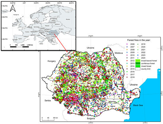
Figure 1.
The study area and the forest fires recorded between 2006 and 2024.
A database with the locations of forest fires in Romania was developed within the “Marin Drăcea” National Institute for Research and Development in Forestry (INCDS) starting in 2006, with the launch of the RO-RISK project, and it has since been continuously updated by adding fire events from each year. The database currently contains detailed records regarding forest fires for the period 2006–2024, with data obtained from the National Forest Administration (RNP) ROMSILVA for state-owned public forests and private forests managed by RNP for the period 2006–2011. Starting from 2012, data have been obtained from the Ministry of Environment, Water, and Forests (MMAP), which centralises fire records for the entire national forest fund, regardless of ownership or management. Records are delivered in tabular format (Excel) and were converted into GIS format (geolocated) based on the geographical coordinates assigned to each fire point (location). The database contains 7434 fires and includes information about fire location, affected area, fire duration, information about the intervention forces mobilised for firefighting (foresters, firefighters, police, gendarmes, and citizens), damages (partial data), and the cause of the fire (according to the European Forest Fire Information System—EFFIS nomenclature) [39], as well as information about the geographical area (e.g., plain, hill, mountain, etc.), forest type (e.g., coniferous, deciduous, mixed, plantation, etc.), and fire type (e.g., litter fire, litter and crown fire—partial data). The study area encompasses the entire territory of Romania, where a national-level map showing the distribution of forest fires was created for the period 2006–2024 (Figure 1).
To model and map areas vulnerable to forest fires at the national level, two machine learning algorithms were used: Maximum Entropy (MaxEnt) and XGBoost.
2.2. Variables Used for the Modelling of Forest Fire Vulnerability
The most relevant independent variables that were considered to determine the degree of vulnerability to forest fires are summarised below (Table 1). A more detailed description of their use is provided in the following paragraphs.

Table 1.
Predictive variables available for the modelling of forest fire vulnerability in Romania.
The Shuttle Radar Topography Mission (SRTM) Digital Elevation Model (DEM) with a 30-m resolution, provided by NASA [40,41], was processed in a GIS system using the SAGA GIS software [50] to obtain topographic variables (elevation; aspect; Topographic Position Index—TPI; Topographic Wetness Index—TWI; slope; valley depth; slope length—LS). The data were generated at a spatial resolution of 250 m using the Pulkovo 1942(58)/Stereo70 projection system.
The main forest types in Romania were grouped into 5 fuel classes according to their pyrotechnic characteristics, which influence the speed and mode of spread of a surface fire, similarly to [15], using the Forest Map by Ecosystem Units [42], in which forests are classified into 140 types of ecosystems that are further grouped into 12 categories. Thus, five relevant forest types were identified based on their distinct fuel properties: coniferous forests, beech (Fagus sylvatica L.) forests, mesophilic oak forests, xerophilic oak forests, and other types of broadleaf forests.
The layer containing the tree cover percentage per unit area was downloaded from the Copernicus platform [43]. The data resolution is 10 m, and the product was obtained from the classification of Sentinel 2 satellite images. The Copernicus program defines tree cover density (TCD) as “the vertical projection of tree crowns onto the horizontal surface of the Earth” and provides information about the proportion of tree crown cover per pixel [51].
Through the GHS-POP geoportal of the European Commission’s Research Centre [44], raster data with a spatial resolution of 100 m was downloaded, referring to the distribution and population density across Romania for the year 2020. Additionally, data regarding the Human Development Index (HDI) developed by [45] was used. They calculated the Gross Domestic Product (GDP) and the Human Development Index globally between 1990 and 2015. The Human Development Index is a composite indicator that measures a country’s progress in terms of health, education, and living standards. The data is presented at a spatial resolution of 5 arc mins (approximately 10 km at the equator) and was downloaded via the Google Earth Engine platform from the GEE Community Catalog repository [52].
From the TOPRO50 dataset provided by the Romanian National Agency for Cadastre and Land Registration—ANCPI [46]—data related to road and railway infrastructure, as well as built-up areas, were extracted, and the following independent variables were generated in raster format at a spatial resolution of 250 m:
- Euclidean distance for the layer of national roads, county roads, and highways;
- Euclidean distance for the layer of communal roads and exploitation roads;
- Euclidean distance for the layer of railway tracks;
- Euclidean distance for the layer of built-up areas.
Afterwards, the newly obtained rasters were resampled to a resolution of 250 m and aligned in terms of extent and geometry with one of the previously obtained topographic variables.
In addition, the Euclidean distances to the boundaries of the following land cover/use classes from the CORINE Land Cover (CLC) 2018 [47] classification were also calculated: irrigated arable land (CLC code 211), secondary pastures (CLC code 321), subalpine vegetation (CLC 322), and transition zones with shrubs (CLC code 324). Rasterization, reprojection, resampling, and geometric alignment with a reference raster were also performed.
The bioclimatic data in raster format were obtained from downscaled versions of the WorldClim and E-OBS datasets [48], which are available for downloading in a public FTP server—ftp://palantir.boku.ac.at/Public/ClimateData/ (accessed on 25 May 2025). Several bioclimatic variables were computed following the methodology of [53] and subsequently used in the analysis:
- Mean annual temperature—bio1;
- Maximum temperature of the hottest month—bio5;
- Mean temperature of the hottest quarter—bio10;
- Mean annual precipitation—bio12;
- Precipitation of the driest quarter—bio17.
The data have a spatial resolution of 0.0083 degrees, which corresponds to approximately 1 km at the equator. The bioclimatic rasters were resampled to a resolution of 250 m and aligned in terms of extent and geometry with one of the previously obtained topographic variables.
In addition, the Canadian Fire Weather Index (FWI) was used—a meteorologically based index that incorporates daily noon values of air temperature, relative humidity, wind speed, and 24-h accumulated precipitation [54].
FWI was calculated for the entire European domain within the framework of the C3S European Tourism project [55], using projections from multiple global climate models (GCMs) that were dynamically downscaled with the RCA4 regional climate model [56]. In this study, annual FWI indicators were used, specifically the multi-model mean, which represents the average FWI derived from all GCM projections under the Representative Concentration Pathway (RCP) 4.5 scenario. The download dataset has a spatial resolution of 0.15 degrees, covers the period 2000–2022, and reflects the number of days per year with moderate fire danger [49].
FWI rasters were resampled to a resolution of 250 m and aligned in terms of extent and geometry with one of the obtained topographic variables.
Among the variables used to assess forest fire vulnerability, fuel type is the only categorical variable; all others are continuous.
Before model development, we evaluated the presence of multicollinearity among the environmental predictors, as this phenomenon can inflate regression variances and reduce model interpretability [57,58,59]. Multicollinearity occurs when several conditioning factors are strongly correlated, potentially biasing model outcomes and overestimating the importance of variables. Therefore, identifying and measuring multicollinearity is considered a critical preliminary step in fire susceptibility modelling.
In this study, we employed a two-step multicollinearity diagnostic approach, which involved pairwise Pearson correlation analysis and the calculation of the Variance Inflation Factor (VIF) and Tolerance (TOL) metrics. VIF quantifies how much the variance of a regression coefficient is inflated due to collinearity with other variables. In contrast, TOL (the reciprocal of VIF) represents the proportion of a predictor’s variance that is independent from the others. As is commonly accepted, VIF values greater than 10 or TOL values below 0.1 were flagged as indicators of problematic multicollinearity [59]. However, this rule should not be treated as a rule of thumb because a high VIF value does not, by itself, invalidate the inclusion of a variable but rather indicates increased variance in its coefficient estimate. As [60] argues, the impact of variance inflation must be interpreted in the context of model objectives and the acceptable level of uncertainty. If the parameter remains theoretically justified and its confidence interval is sufficiently narrow for this study’s purpose, even high VIF values (e.g., >10) may be tolerated without compromising the model’s reliability.
Pearson correlation coefficients were first calculated between all continuous initial predictors derived from topographic, climatic, vegetation, and anthropogenic sources. Variables involved in strong pairwise correlations (|r| > 0.8) were flagged for potential removal. Subsequently, VIF and TOL values were computed on the filtered variable set to ensure that no remaining predictors exhibited unacceptable levels of collinearity.
2.3. Maximum Entropy Model
Maximum Entropy (MaxEnt) is a machine learning approach that relies exclusively on presence-only data. It estimates the relative suitability of locations by contrasting the environmental conditions at known fire occurrence sites with those from a randomly sampled background across the entire study region [61]. The algorithm aims to find the probability distribution of Maximum Entropy (i.e., closest to uniform), subject to constraints imposed by the observed data, thereby avoiding assumptions not supported by evidence. Entropy, in this context, quantifies the uncertainty of a probability distribution [62]. In MaxEnt, the probability of ignition occurrence is assigned to each location based on how well it satisfies the average environmental conditions observed at the presence locations [61]. Each site receives a non-negative probability, and the sum of all assigned probabilities across the landscape equals one. The model is constrained such that the average value of each predictor across the predicted distribution closely matches its empirical mean at the observed fire locations [62]. Among all possible distributions that meet these constraints, MaxEnt selects the one that is most uniform, representing the least biased inference given the available information [61]. Additionally, MaxEnt can accommodate complex, nonlinear relationships between predictors and fire presence by enabling different feature types—such as linear, quadratic, hinge, or product functions—thus enhancing the flexibility and expressiveness of the model [63].
The MaxEnt application allows the user to generate the possible distribution through various parameters that can be used for learning and generating graphical results, while also producing valid results based on the AUC (Area Under the Curve) measurement and the jackknife method, which is a resampling technique helpful in estimating bias and variance.
2.3.1. Model Optimization
The MaxEnt model was run using version 3.4.4 of the dedicated software [64]. To optimise MaxEnt performance and reduce overfitting, we implemented a structured hyperparameter tuning procedure using the dismo: maxent function [65] in R Core Team (2024) [66]. We tested combinations of feature classes (linear, quadratic, hinge, and product) and regularisation multipliers (RM = 0.05, 0.5, 1, 2, 3, 4), explicitly disabling the autofeature option to control feature inclusion. For each configuration, we evaluated model performance using the training AUC (Area Under the Curve) and the True Skill Statistic (TSS). Model selection was based on the highest AUC value, while TSS was used as a complementary diagnostic. All models were trained with a fixed random seed (randomseed = true) to ensure the full reproducibility of the results, including AUC, TSS, and response curves. Background points were sampled only within areas containing valid fuel type information (i.e., non-null fuel_type values), representing zones where wildfires are ecologically plausible. This constraint aligns with best practices in ecological niche modelling, which recommend restricting the background to the accessible area [67] to avoid bias and inflated accuracy metrics [68]. Final predictions were also masked in forest combustible regions to ensure consistency between training and projection.
The predictive performance of the MaxEnt model is commonly assessed using the Receiver Operating Characteristic (ROC) curve and its associated Area Under the Curve (AUC) metric. The ROC curve plots the actual positive rate against the false positive rate, and the AUC summarises this relationship into a single value between 0 and 1. A score of 0.5 suggests random prediction, while a value of 1.0 indicates perfect discrimination. Typically, an AUC below 0.6 reflects weak predictive capability; values between 0.6 and 0.7 are considered poor, 0.7 to 0.9 are considered moderate, and scores above 0.9 suggest high predictive accuracy [69].
2.3.2. Uncertainty Estimation
To quantify predictive uncertainty associated with MaxEnt parameter settings, we computed a pixel-wise standard deviation of logistic outputs generated by all model configurations tested during hyperparameter tuning. Each model corresponded to a distinct combination of feature classes (linear, quadratic, hinge, and product) and regularisation multipliers. The resulting standard deviation raster was normalised to a 0–1 scale and exported as a GeoTIFF. To facilitate interpretation, the continuous uncertainty values were reclassified into five equal-width classes: [0.0–0.2], [0.2–0.4], [0.4–0.6], [0.6–0.8], and [0.8–1.0]. This spatially explicit uncertainty map highlights areas of low versus high model agreement, offering a practical assessment of predictive robustness across the study area.
2.4. eXtreme Gradient Boosting Model
eXtreme Gradient Boosting (XGBoost) is an open-source machine learning algorithm that implements an efficient and scalable version of gradient-boosted decision trees [70]. Its ability to handle structured data, capture complex nonlinear relationships, and scale across large datasets makes it particularly well-suited for environmental modelling applications, including wildfire susceptibility assessment. In this domain, XGBoost has proven to be a powerful predictive tool capable of integrating diverse geospatial and environmental inputs—such as topography, vegetation indices, meteorological variables, and human activity indicators—to generate accurate models of fire risk. Recent studies have demonstrated the strong performance of the algorithm in fire vulnerability mapping [12,71]; therefore, it was selected in this study. A distinguishing feature of XGBoost is its use of regularised learning, which includes both L1 (Lasso) and L2 (Ridge) penalties [72]. This helps prevent overfitting and improves the model’s generalisation capacity, particularly when working with high-dimensional environmental datasets. The algorithm also employs a second-order Taylor expansion of the loss function, allowing it to leverage both gradients and Hessians for more accurate and faster convergence compared to traditional gradient boosting techniques. Its support for parallel and distributed computing enables it to scale efficiently when applied to large and heterogeneous spatial datasets [73]. Moreover, XGBoost includes a sparsity-aware learning mechanism, making it well-equipped to handle missing or incomplete data, a common issue in ecological and geospatial research. It also allows users to define custom loss functions and evaluation metrics, offering the flexibility needed to tailor the model to specific policy or management needs, such as distinguishing between vulnerability levels or aligning with fire prevention priorities.
Unlike MaxEnt, which is designed to operate with presence-only data and compares known occurrences against background environmental conditions, XGBoost is a supervised learning algorithm that requires both presence and absence data to function effectively. In wildfire susceptibility modelling, this means that in addition to locations where fires have occurred, the model also needs information on areas where fires were absent or not recorded. If accurate absence data are unavailable, pseudoabsence points must be generated to enable the application of XGBoost. This distinction has important implications for model design and data preparation. In this study, a 1 km buffer was selected to generate non-fire points, ensuring sufficient spatial separation from fire occurrence points while maintaining ecological relevance within forested areas. Given the 250 m resolution of the dataset and the heterogeneous distribution of fire incidents across Romania, with some high-density “hotspot” counties, a 1 km buffer effectively minimises overlap between presence and absence points, particularly in less dense areas. This distance, equivalent to approximately four pixels, strikes a balance between capturing distinct environmental conditions for non-fire points while avoiding the inclusion of non-forested or irrelevant land cover types, which could occur with a larger buffer.
The modelling workflow for the XGBoost approach consisted of two main stages: (i) training and evaluating the model using presence–absence fire occurrence data and (ii) generating a continuous spatial vulnerability map through prediction.
The training dataset for the XGBoost model was constructed using georeferenced fire occurrence points (presence) and stratified pseudoabsence points, which were generated outside a 1 km buffer around historical fire locations to minimise overlap. Absence points were sampled randomly, stratified by fuel type based on a five-class vegetation fuel map, ensuring proportional ecological representation. A minimum distance of 300 m between absence points was enforced to minimise spatial clustering and sampling bias. For each point, values of predictive environmental variables were extracted from a set of raster layers. These variables included topographic metrics (elevation, slope, aspect, TWI, TPI, valley depth, and LS-Factor), vegetation structure (tree cover and fuel type), climatic variables (bioclimatic indices and Fire Weather Index), anthropogenic factors (distance to roads, buildings, pastures, and agricultural land), and demographic indicators (population density and Human Development Index).
2.4.1. Model Optimization
To optimise the performance of the XGBoost classifier and improve generalisation, we applied two hyperparameter tuning strategies: an exhaustive grid search using GridSearchCV [74] and Bayesian optimisation via BayesSearchCV from the scikit-optimise library [75]. Both approaches employed five-fold stratified cross-validation and used the Area Under the ROC Curve (AUC) as the primary evaluation metric. The grid search evaluated 48 predefined combinations of key hyperparameters, including max_depth, learning_rate, n_estimators, subsample, and colsample_bytree. Bayesian optimisation explored the same parameters over a broader, continuous search space, using a probabilistic surrogate model to refine the search iteratively. Both GridSearchCV and BayesSearchCV performed hyperparameter tuning using internal 5-fold cross-validation, enabling the iterative evaluation and optimisation of model performance on validation subsets. For each tuning strategy, the best-performing configuration was selected based on the highest mean AUC across folds. The F1 score was calculated as a secondary metric to assess classification balance. The two resulting models from each strategy were subsequently compared based on their evaluation metrics, and the one with superior performance was retained for final interpretation and used to generate the probability and uncertainty maps.
The best model was finally evaluated using several metrics, including the Area Under the Receiver Operating Characteristic Curve (AUC), F1 score, accuracy, precision, recall, and confusion matrix. To assess variable importance and interpret model predictions, SHAP (SHapley Additive exPlanations) values were computed [76], allowing both global and local explanations of model behaviour.
These evaluation metrics for the XGBoost model offer complementary insights into the model’s classification ability, such as the following: (i) precision represents the proportion of true positives among all predicted positives, measuring how many predicted fire occurrences were correct; (ii) recall (also known as sensitivity) indicates the proportion of actual fires that the model correctly identified; (iii) the F1 score is the harmonic mean of precision and recall, providing a balanced assessment that penalises significant disparities between them.
Using the trained model, predictions were extended spatially to the entire study area. All raster layers used during model training were spatially aligned and stacked into a multi-band array, with a mask applied to restrict predictions to forested pixels (tree cover > 0). For each valid pixel, the predictor values were reshaped and passed to the trained XGBoost model to compute the probability of fire occurrence. The resulting continuous raster of predicted probabilities (ranging from 0 to 1) was saved as a GeoTIFF file. Subsequently, this raster was reclassified into five vulnerability classes using equal-width intervals: [0.0–0.2], [0.2–0.4], [0.4–0.6], [0.6–0.8), and [0.8–1.0]. This classification facilitates interpretation and supports practical applications in fire management planning.
2.4.2. Uncertainty Estimation
To assess spatial prediction uncertainty in the XGBoost model, we calculated the pixel-wise standard deviation across all prediction maps generated during hyperparameter tuning. Each prediction corresponded to a unique combination of tuning parameters applied to the same set of 20 environmental rasters. The resulting standard deviation map was masked to include only forested areas (fuel_type > 0) and then reclassified into five equal-width uncertainty classes, consistent with the MaxEnt model. This map highlights regions of greater prediction variability and provides a spatial assessment of model robustness.
The dependent variable used in the MaxEnt model consisted of fire event locations provided in .csv format, containing X and Y coordinates in the Pulkovo 1942(58)/Stereo70 projection (EPSG:3844). The software requires the modelling data to be in ASCII format, so all predictive variables were converted to this format (they were initially generated in GeoTiff format). All independent variables must have precisely the same number of rows and columns, share the exact spatial resolution (in our case, 250 m), be perfectly aligned with each other, and be in the same projection system (EPSG 3844). The value for fields with missing data was set to −9999 for all predictive variables. For each variable, the type must be specified as either continuous or categorical.
2.5. Accuracy Assessment of the Modelled Forest Fire Vulnerability Maps
To assess the external validity of the fire vulnerability maps generated with MaxEnt and XGBoost, we used active fire detections from the Visible Infrared Imaging Radiometer Suite (VIIRS) sensor onboard the NASA Suomi NPP satellite [77]. VIIRS provides near-real-time active fire data at a spatial resolution of 375 m, accessible via the Fire Information for Resource Management System (FIRMS). We downloaded the full archive of VIIRS fire detections across Romania for the period 2012–2024 and applied a filtering procedure to retain only reliable observations. Specifically, we retained fire points with a fire radiative power (FRP) of ≥3 MW, scan angle of ≤0.6, and a confidence level classified as either “high” or “nominal” (i.e., excluding “low” confidence detections). After filtering, a total of 150,426 fire points remained. These validated fire points were spatially intersected with the vulnerability maps produced by each modelling approach (MaxEnt and XGBoost). For each map, we extracted the vulnerability class (1–5) for forests at the location of every VIIRS point. We then calculated the percentage distribution of fire detections across vulnerability classes for each model, which served as an independent validation metric.
The flowchart below provides a synthesised overview of the methodological framework described in Section 2, detailing the sequential steps undertaken for data acquisition, processing, model calibration, and the generation of forest fire vulnerability and uncertainty maps using MaxEnt and XGBoost approaches (Figure 2).
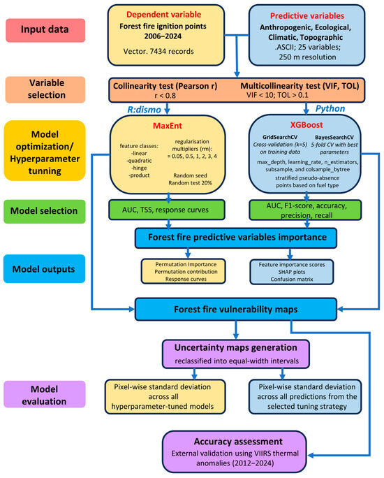
Figure 2.
Overview of the methodological workflow applied in this study.
3. Results
3.1. Variable Selection
Both MaxEnt and XGBoost models require the same set of independent variables to predict forest fire vulnerability. Following the methodology, all variables were resampled to a spatial resolution of 250 m and standardised in terms of extent and geometry to ensure spatial consistency (Figure 3).
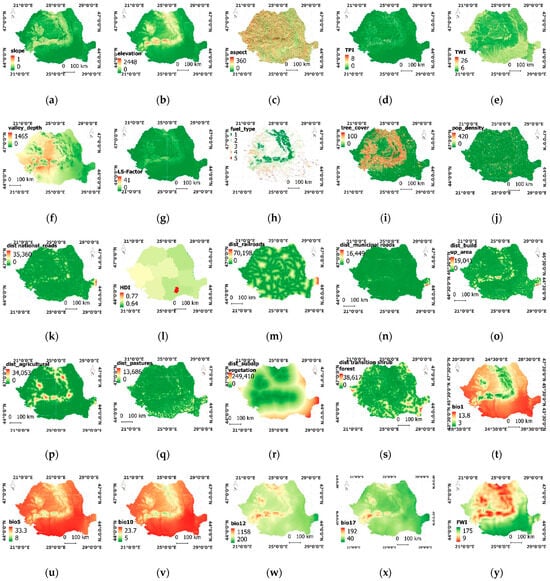
Figure 3.
The most relevant predictive variables available for the modelling of forest fire vulnerability in Romania: (a)—slope; (b)—elevation; (c)—aspect; (d)—TPI; (e)—TWI; (f)—valley depth; (g)—slope length; (h)—type (material) of forest fuel; (i)—tree cover density; (j)—average population density; (k)—HDI; (l)—Euclidean distance for national county roads, highways vector layer; (m)—Euclidean distance for communal roads, exploitation roads vector layer; (n)—Euclidean distance for railways vector layer; (o)—Euclidean distance for built-up areas vector layer; (p)—Euclidean distance for irrigated arable lands (CLC211); (q)—Euclidean distance for secondary pastures (CLC231); (r)—Euclidean distance for subalpine vegetation (CLC322); (s)—Euclidean distance for shrubland transition zones (CLC324); (t)—Bio1; (u)—Bio5; (v)—Bio10; (w)—Bio12; (x)—Bio17; (y)—FWI.
The initial Pearson correlation matrix revealed several strong associations among all continuous candidate predictors (Figure 4), including bio1–FWI (r = 0.86), elevation–bio1 (r = −0.95), elevation–bio12 (r = 0.80), and bio10–bio5 (r = 0.93). Based on these findings and ecological interpretability considerations, five variables were excluded from the modelling process: bio1, bio5, bio10, bio12, and LS-Factor. These predictors either presented overlapping ecological content or exhibited strong collinearity with others, introducing redundancy in the model’s structure.
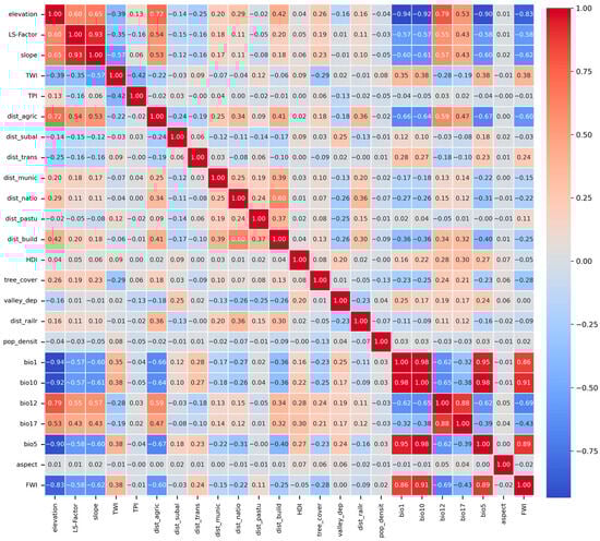
Figure 4.
Pearson correlation matrix of initial predictors (variable abbreviations are consistent with those presented in Table 1).
The remaining 19 predictors (excluding the categorical variable fuel_type, which was not included in the Pearson correlation analysis) were further evaluated using VIF and TOL metrics. As shown in Table 2, all retained variables had VIF values below 10 and TOL values above 0.1. The highest VIF was observed for elevation (VIF = 8.56), indicating that multicollinearity was substantially reduced following the selection procedure. The final predictor set was thus deemed suitable for inclusion in the MaxEnt and XGBoost modelling frameworks.
Table 2.
Multicollinearity analysis results.
Although a strong negative correlation was observed between elevation and FWI (r = −0.83), elevation was retained in the final set of predictors due to its distinct ecological and physical relevance. While FWI represents a dynamic fire danger index derived from recent weather conditions, elevation is a fundamental topographic driver that shapes long-term vegetation patterns, microclimates, and fuel structure. The two variables, though related, capture different temporal and ecological dimensions of fire risk. Furthermore, elevation has been shown to influence fire behaviour independently of weather-derived indices in mountainous and transitional landscapes. Therefore, its inclusion was considered justified despite its statistical association with FWI.
3.2. MaxEnt Model
A total of 24 MaxEnt models were fitted by combining four feature class configurations (linear; linear + quadratic; linear + quadratic + hinge; linear + quadratic + hinge + product) with six regularisation multipliers (RM = 0.05, 0.5, 1, 2, 3, 4). Model performance was evaluated using both AUC and TSS metrics, with values ranging from 0.728 to 0.774 (AUC) and 0.356 to 0.421 (TSS). The highest AUC (0.774) was achieved by the model using all feature classes and RM = 0.05. However, upon the visual inspection of response curves, this model exhibited several biologically implausible patterns, including abrupt spikes, irregular inflexions, and extreme predictions—signs indicative of overfitting. By contrast, the same feature combination with RM = 0.5 produced smoother and more ecologically interpretable response curves, while maintaining comparable predictive performance (AUC = 0.758). Therefore, this model was retained for final analysis, as it provided a more appropriate trade-off between discrimination power and ecological plausibility. This decision aligns with previous findings on the importance of regularisation in avoiding model overfitting when using complex feature sets [78,79].
The predictive performance of the selected MaxEnt model (RM = 0.5, LQHP) was further confirmed by the ROC curve, which yielded an AUC of 0.770 for the training dataset and 0.758 for the test dataset. Both values exceed the commonly accepted threshold of 0.7, indicating that the model achieved moderate discrimination capacity and met the reliability standards for ecological predictive modelling (Figure 5).
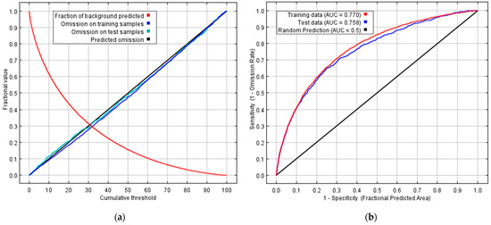
Figure 5.
Performance of the MaxEnt model: (a) omission rate and predicted area as a function of the cumulative threshold and (b) ROC (Receiver Operating Characteristic) curve.
The result of the MaxEnt model (Table 3) presents the contribution and importance of variables through two indicators: Percent Contribution and Permutation Importance.
Table 3.
Contribution and importance of the prediction classes for the MaxEnt model.
The Percent Contribution shows the contribution of each explanatory variable to the construction of the model based on the training algorithm. This percentage reflects how much a given variable has contributed to the creation of the model’s predictions. The algorithm adjusts the weights of the variables during training to maximise entropy, and this indicator provides insight into the relative importance of each variable in the process. A variable with a high value has significantly influenced the model’s predictions, indicating that the model relies heavily on that variable. A variable with a low percentage has a smaller contribution and may have a minor impact on the predictions. For example, if we study the distribution of a species, a variable such as temperature might have a 50% contribution, indicating that temperature variations most explain the species’ presence in different locations.
The Permutation Importance indicator measures the model’s sensitivity to a variable by evaluating the impact of that variable on model performance through permuting (reshuffling) the values of the respective variable. Permutation Importance indicates the extent to which the model’s performance (e.g., AUC) deteriorates when the values of a variable are randomly permuted. A higher value indicates that the variable is significant for the model. A low value suggests that the model is not very sensitive to that variable and may partially ignore it. For example, if the average annual temperature has a high Permutation Importance value, we can conclude that the model is sensitive to temperature variations, and removing or altering this variable would significantly degrade the accuracy of the predictions.
The relative contribution and importance of the predictive variables in the final MaxEnt model (RM = 0.5, LQHP) are shown in Table 3. Two complementary metrics were used to evaluate the role of each variable: Percent Contribution and Permutation Importance. Percent Contribution reflects the influence of each variable during model training based on how often and how strongly it is used in the model’s decision rules. Permutation Importance, in contrast, quantifies the drop in model performance (e.g., AUC) when the values of a variable are randomly permuted and, thus, indicates the model’s dependence on that variable for accurate prediction.
At the group level, the most influential predictors in terms of Percent Contribution were anthropogenic variables (40.7%), followed by vegetation (24.7%), climatic factors (17.4%), and topography (17.1%). In contrast, when ranked by Permutation Importance, topographic variables dominated (45.5%), followed by climatic factors (28.8%), anthropogenic factors (23.4%), and vegetation (2.2%).
Among individual variables, fuel_type had the highest Percent Contribution (22.6%) but very low Permutation Importance (0.5%), indicating that although the variable was heavily used during model training, it had a limited effect on predictive performance when permuted. This suggests that fuel_type may have interacted strongly with other variables during training but was not essential for final model accuracy. The variable with the highest Permutation Importance by far was elevation (32.0%), highlighting its dominant role in shaping the model’s predictive surface. The Fire Weather Index (FWI) also had substantial influence (Contribution = 16.4%; Permutation = 25.8%), underscoring the importance of seasonal fire danger conditions. Anthropogenic variables such as dist_agric (i.e., distance to arable lands) and dist_build (i.e., distance to built-up areas) had a moderate influence under both metrics, suggesting that proximity to human-altered landscapes is relevant to fire risk, with the presence and actions of human factors serving as catalysts for fire ignition.
Overall, the variable importance analysis reveals a shift in dominance depending on the metric: Percent Contribution emphasises how the model was trained, while Permutation Importance better reflects predictive dependency. The most influential predictors in terms of actual predictive performance were elevation, FWI, and bio12 (precipitation), highlighting the strong role of topography and climate in determining forest fire vulnerability across the study area.
The response curves generated for each environmental predictor using the MaxEnt model (Figure 6) illustrate that the relationship between fire occurrence and environmental variables is generally nonlinear and varies across gradients. These effects are not uniform but exhibit complex, often nonlinear dynamics shaped by multiyear trends in temperature, precipitation, aridity, land use, proximity to infrastructure, and topographic features. Additionally, the contribution of each variable changes with its value range, and correlations between predictors can vary considerably. It is commonly understood that intervals where the predicted probability surpasses 0.5 are those most likely associated with fire occurrence. Each environmental factor tends to exhibit a specific response range that increases the likelihood of fire.
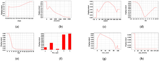
Figure 6.
Response curves of the MaxEnt model for the independent variables: (a)—slope; (b)—elevation; (c)—aspect; (d)—TPI; (e)—TWI; (f)—type (material) of forest fuel; (g)—tree cover density; (h)—average population density; (i)—HDI; (j)—Euclidean distance for national county roads, highways vector layer; (k)—Euclidean distance for communal roads, exploitation roads vector layer; (l)—Euclidean distance for railways vector layer; (m)—Euclidean distance for built-up areas vector layer; (n)—Euclidean distance for irrigated arable lands (CLC211); (o)—Euclidean distance for secondary pastures (CLC231); (p)—Euclidean distance for subalpine vegetation (CLC322); (q)—Euclidean distance for shrubland transition zones (CLC324); (r)—Bio12; (s)—FWI.
In the case of individual factors, various environmental variables have optimal intervals related to their effects on contributing to the probability of fire outbreak and spread. Fuel type is the only categorical input variable in the model. According to the model (Figure 6f), the most vulnerable forests to fires are thermophilic oak forests, followed by the “other broadleaf forests” group. Next are the beech forests and mesophilic oak, which are the least vulnerable to fires, followed by coniferous forests. The results of applying this model can also confirm this.
From the interpretation of the individual response curves, it is highlighted that the closer the distance to anthropogenic elements (e.g., agricultural land, built-up areas), the higher the probability of fire. Land aspect has a clear response to fires, with its curve having a typical bell shape and exhibiting maxima for terrains with sunny slopes (S, SE, and SW), and it decreases as the level of land shading increases.
In the case of elevation, the graph shows a very high susceptibility to fires in low-altitude areas, with a peak around an altitude of 400 m, after which it decreases sharply and even flattens out around the 1000 m value.
The MaxEnt model provides a zoning of the probability of occurrence of the modelled variable (in our case, forest fires) in .ascii format, with values ranging from 0 to 1. The probability predictions were classified into five separate categories (very low, low, moderate, high, and very high) with the equal interval classification method (Figure 7a). The uncertainty map of the vulnerability predictions is presented in Figure 7b.
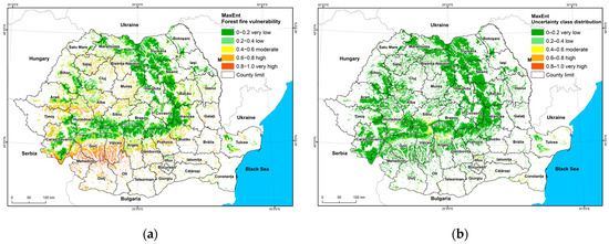
Figure 7.
Forest fire vulnerability map at the national scale (a) and corresponding uncertainty map (b), both generated using the Maximum Entropy (MaxEnt) model.
3.3. XGBoost Model
The predictive performance of the XGBoost classifiers obtained through hyperparameter tuning with GridSearchCV and BayesSearchCV was compared using several standard metrics, including the Area Under the ROC Curve (AUC), accuracy, precision, recall, and F1 score. The best model from the grid search procedure achieved an AUC of 0.988, indicating excellent discrimination between fire and non-fire locations. This model also exhibited high classification performance, with an accuracy of 0.947, precision of 0.945, recall of 0.947, and F1 score of 0.947. In contrast, the best model resulting from Bayesian optimisation achieved an AUC of 0.841, with a corresponding accuracy of 0.766, precision of 0.772, recall of 0.745, and F1 score of 0.763.
A more detailed classification report confirmed the superior performance of the grid search approach across all metrics and both fire presence and absence classes (Table 4). As a result, the XGBoost model tuned via GridSearchCV was retained for subsequent analyses and used to generate the fire vulnerability prediction map and associated uncertainty layers.
Table 4.
Performance metrics and classification report for the XGBoost model for both grid search and Bayesian optimisation hyperparameterization approaches. Metrics are based on presence–absence classification using independent validation data.
The macro-average calculates the mean of the individual metric scores across all classes, treating each class equally regardless of its size. In contrast, the weighted average accounts for the number of samples in each class when averaging the metrics, giving more importance to dominant classes. In this analysis, both macro-averages and weighted averages for precision, recall, and F1 score were approximately 0.95, confirming the balanced and consistent performance of the model across both classes (Figure 8).
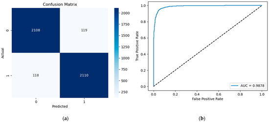
Figure 8.
Confusion matrix (a) and AUC performance (b) of the XGBoost algorithm optimised with grid search.
To identify the key predictors influencing forest fire susceptibility, we examined the feature importance scores provided by the optimised XGBoost model (Figure 9). The most influential variables were the Fire Weather Index (FWI), forest fuel type, elevation, and distance to agricultural lands, highlighting the importance of climatic fire danger conditions, vegetation structure, and human-altered landscapes. Topographic factors, such as slope and valley depth, also contributed substantially, reflecting their significant role in fire spread dynamics. Notably, variables such as distance to built-up areas and HDI further emphasised the relevance of anthropogenic exposure.
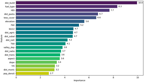
Figure 9.
Importance scores of conditioning factors (variable abbreviations are consistent with those presented in Table 1).
To enhance model interpretability, SHapley Additive exPlanations (SHAPs) were employed. The SHAP summary plot (Figure 10a) confirmed the dominant contribution of FWI, fuel type, and elevation to fire susceptibility. Higher values of FWI, elevation, and slope were consistently associated with increased fire probability. In contrast, certain fuel types and high vegetation cover showed suppressive effects. The SHAP dependence plot for the fuel_type variable (Figure 10b) revealed distinct patterns across vegetation classes. Coniferous forests (Fuel Type 1) and thermophilous oak forests (Fuel Type 4) had the highest positive SHAP values, indicating increased fire susceptibility, while beech forests (Fuel Type 2) and mesophilous oak forests (Fuel Type 3) were associated with lower predicted probabilities of fire. These results highlight the pivotal role of forest composition and flammability in shaping fire occurrence patterns.
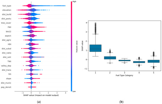
Figure 10.
SHAP summary plots for modelling using XGBoost (a) and SHAP for the fuel types predictive category (b) (variable abbreviations are consistent with those presented in Table 1).
The fire vulnerability map generated with the optimised XGBoost model is presented in Figure 11a. The probabilities of fire occurrence were reclassified into five vulnerability classes—very low, low, moderate, high, and very high—using the same equal-width classification scheme applied to the MaxEnt prediction. This spatial product highlights areas of elevated fire risk and can support operational decision-making in forest protection planning. The uncertainty map of the vulnerability predictions is presented in Figure 11b.
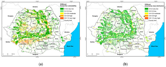
Figure 11.
Forest fire vulnerability map at the national scale (a) and corresponding uncertainty map (b), both generated using the eXtreme Gradient Boosting (XGBoost) model.
3.4. Assessment of the Modelled Forest Fire Vulnerability Maps
Several important insights can be drawn from the spatial distribution of the forest fire vulnerability classes across the study area. While there are notable differences between the classifiers in the proportions assigned to the low and very low categories, the results are broadly consistent for the moderate, high, and very high vulnerability levels (Figure 12a). According to the MaxEnt model, the largest share of the territory falls within the low (32.6%) and very low (31.4%) vulnerability classes. In contrast, the XGBoost model classifies 34.87% of the area as very low and 29.56% as low. The proportion of moderate vulnerability areas is nearly identical between the two models: 18.52% for MaxEnt and 18.24% for XGBoost. For high vulnerability, MaxEnt assigns 10.61% of the area, slightly less than the 11.84% identified by XGBoost. Lastly, very high vulnerability areas represent 6.86% of the territory under MaxEnt and 5.49% under XGBoost.
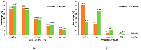
Figure 12.
Spatial distribution of forest fire vulnerability classes (a) and associated uncertainty levels (b) for the MaxEnt and XGBoost models.
Regarding the spatial uncertainty associated with each model (Figure 12b), the MaxEnt map generally displays lower uncertainty values across most of the study area, with high uncertainty concentrated in peripheral zones and areas of steep terrain. In contrast, the XGBoost uncertainty map exhibits more dispersed areas of moderate to high variability, particularly in ecotonal regions and areas with mixed fuel composition. These patterns reflect the different ways in which each model handles predictor interactions and feature complexity during training.
The external validation using VIIRS active fire detections supports the relevance of both models. The highest proportions of fire points fall within the “high” and “very high” vulnerability classes for both MaxEnt and XGBoost (Figure 13). This concordance suggests that the predicted vulnerability surfaces align well with actual fire occurrence patterns, despite methodological differences between the classifiers. The validation results highlight the practical utility of the maps for operational fire risk assessment.
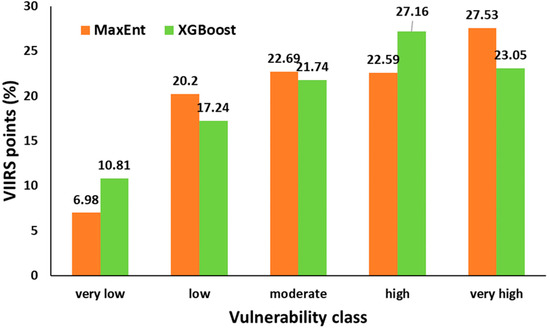
Figure 13.
Percentage distribution of VIIRS active fire detection points (2012–2024) across the five vulnerability classes predicted by the MaxEnt and XGBoost models. The highest proportions of VIIRS fire points are located in the “high” and “very high” vulnerability classes for both models, supporting the spatial relevance of the predicted susceptibility maps.
4. Discussion
In Romania, forest fires represent one of the most probable natural hazards, even if their overall destructive impact remains moderate when compared with other hazard types [17]. Nevertheless, the number of fire events has risen considerably since 2000, with record-breaking fire activity registered in 2012 and 2022, years that marked the highest values for both fire occurrence and total surface affected.
In this study, the equal interval classification method was used to divide the forest fire vulnerability values across Romania into five levels (Figure 5), as was also carried out in the study by [15]. Other authors have grouped them according to the natural breaks criterion [80] or quartiles [7]. The five subdivisions with different vulnerability levels were classified as areas with very low vulnerability (0–0.2), low vulnerability (0.2–0.4), medium vulnerability (0.4–0.6), high vulnerability (0.6–0.8), and very high vulnerability (0.8–1.0).
From a spatial perspective, both models consistently indicate that the areas most vulnerable to forest fires are located in the Sub-Carpathian and lowland regions, where forests are interspersed with agricultural lands, pastures, and human settlements. These landscapes are particularly vulnerable to climatic stressors, such as prolonged droughts and heat waves, which exacerbate fire susceptibility. A strong correlation emerges between fire incidence and seasonal land management practices. In the spring, fires are frequently set to clear plant debris in pastures and orchards, especially in hilly areas. In contrast, the peak of fire activity shifts to the lowlands and Dobrogea in the summer, mainly due to stubble burning. Additionally, mountainous regions also experience increased fire occurrences during the summer, driven by the heightened human presence associated with tourism. The extensive and contiguous forested areas within the Carpathians exhibit predominantly low and very low vulnerability levels. Although these forests have a high proportion of resinous species, such as Norway spruce and fir—known for their increased flammability—they are less affected by forest fires, primarily due to limited anthropogenic ignition sources in these remote, less accessible areas.
The geographic distribution of vulnerability reveals a distinct concentration of high-risk areas in southwestern Romania, particularly in the counties of Mehedinți, Gorj, Vâlcea, Dolj, and Olt. Notably, in Mehedinți and Gorj, high vulnerability is confined to lowland and hilly areas, decreasing toward the mountainous zones. These findings are consistent with previous research [14,81], which identified similar hotspots using kernel density, Random Forest, and logistic regression. The repeated identification of Sub-Carpathian regions as fire-prone confirms the combined influence of vegetation type, land use, and anthropogenic pressures on fire vulnerability patterns across Romania.
Beyond the spatial patterns revealed, a comparative analysis of the two modelling approaches—Maximum Entropy (MaxEnt) and eXtreme Gradient Boosting (XGBoost)—offers valuable insights into their predictive performance, variable importance, and methodological strengths and limitations.
Both models used the same set of environmental predictors, ensuring a consistent basis for comparison. Among the most influential predictors in both methods are climatic variables, particularly the Fire Weather Index (FWI), followed by forest fuel type and topographic variables such as slope and elevation. Anthropogenic factors such as proximity to roads, built-up areas, and pastures also play a significant role, confirming the strong interaction between human activity and fire occurrence.
In terms of predictive power, XGBoost achieved a very high AUC (0.988), indicating excellent classification ability and outperforming MaxEnt, which yielded a moderate test AUC of 0.758. While MaxEnt falls within the commonly accepted threshold for moderate predictive accuracy (0.7–0.9), it slightly underperforms compared to analogous wildfire susceptibility modelling efforts in other regions [12,13,71]. The substantial difference between the two models suggests that the machine learning-based classifier is better suited for capturing complex interactions and nonlinear relationships among predictors. Several factors may explain the discrepancy: (i) the static nature of input variables, which do not account for temporal dynamics; (ii) MaxEnt’s reliance on presence-only data, which can introduce bias in background selection; and (iii) the capacity of XGBoost to incorporate richer decision structures and benefit from a balanced set of presence and pseudoabsence samples.
In comparative studies, similar AUC values have been reported: for instance, an AUC of 0.91 for XGBoost in Guilin, China [71], and above 0.85 for MaxEnt and XGBoost in the Mediterranean region of Turkey [12,13]. For example, in the Mediterranean region of Türkiye, [82] applied XGBoost to assess forest fire susceptibility, achieving AUC values ranging from 0.85 to 0.88. Similarly, [63] demonstrated that MaxEnt could effectively capture fire-prone patterns across varied ecosystems in the Western United States, particularly where weather and vegetation interact strongly with fire probability. Comparable research conducted in Hawaii by [59] reported AUC values of 0.916 for XGBoost and up to 0.927 for hybrid metaheuristic versions. In contrast, a MaxEnt-based study in Nepal [83] achieved an AUC of 0.861, classified as “very good” performance. Furthermore, an explainable XGBoost model developed in Guizhou Province, China [38], reached an AUC of 0.983 using SHAP-based interpretability, revealing that proximity to villages, air humidity, and vegetation surface temperature were the most influential predictors.
These reported accuracies likely reflect region-specific fire regimes with more consistent spatial patterns or the availability of higher-resolution dynamic input data. Conversely, the moderate AUC values observed in Romania may stem from the complex mosaic of ecological zones, socio-economic factors, and diverse fire ignition sources, which introduce heterogeneity that challenges model generalisation. This variability emphasises the importance of further refining modelling approaches to capture spatial and temporal complexities inherent in Romanian fire dynamics.
One plausible explanation is the high regional variability in fire activity across Romania, influenced not only by environmental conditions but also by divergent socio-economic and land management practices. A representative example is the Dobrogea region in southeastern Romania, characterised by arid, steppe-like conditions and xerophilous oak forests. Despite this ecological predisposition to fires, the frequency of forest fire events is comparatively low, with both models placing the forests in this region in low and very low vulnerability classes. Field knowledge indicates that local communities implement effective fire prevention strategies, such as maintaining mineralised strips between agricultural fields and forests. This localised human behaviour, not easily captured by static predictors, may partially explain why vulnerability levels are lower than expected in such areas.
One methodological limitation of the present study is the absence of explicit spatial cross-validation or spatial partitioning during model evaluation. While we employed a stratified random train–test split to ensure the proportional representation of ecological conditions, this approach does not fully account for the spatial autocorrelation inherent in fire occurrence data. As a result, predictive performance metrics such as AUC may be slightly overestimated due to the spatial proximity between training and testing samples. Future research should incorporate spatial cross-validation techniques, such as block cross-validation or spatial k-fold methods, to better assess model generalisability and reduce the influence of spatial clustering. Such approaches would provide more conservative and spatially realistic estimates of model performance and transferability, especially in heterogeneous landscapes.
This spatial heterogeneity suggests a limitation of both MaxEnt and XGBoost in their current configurations, as neither model accounts for spatially varying relationships between predictors and fire susceptibility. While MaxEnt operates under the assumption of a uniform background and MaxEnt presence-only modelling and XGBoost assumes global predictor–response relationships across the landscape, neither can accommodate non-stationary spatial processes. In this context, the use of Geographically Weighted Regression (GWR) could offer a valuable alternative [84,85]. GWR allows model coefficients to vary across space, capturing local variations in predictor influence and potentially improving predictive performance in regions with heterogeneous fire behaviour. Despite these limitations, both models offer distinct advantages. MaxEnt is particularly well-suited for presence-only datasets and performs robustly even with limited input data. It is easy to implement and interpret, which makes it widely used in ecological applications. However, it tends to overpredict in areas with environmental conditions similar to presence points, mainly because absence information is lacking. In contrast, XGBoost is a powerful ensemble learner capable of modelling complex nonlinear relationships and interactions between predictors. Its ability to handle missing data, reduce overfitting through regularisation, and deliver interpretable outputs via SHAP values makes it a state-of-the-art tool for large-scale fire vulnerability assessments.
Other models, such as Random Forest (RF), Support Vector Machines (SVMs), or Generalised Linear Models (GLMs), have also been used in wildfire susceptibility mapping. Random Forest, for instance, has shown strong performance in several studies due to its robustness and ease of interpretation [10,34], but it may struggle with imbalanced datasets and lacks probabilistic output. SVMs are effective in high-dimensional spaces but are sensitive to parameter tuning and can be less interpretable. MaxEnt, while often outperformed by machine learning classifiers in terms of accuracy [11,71], remains useful when only presence data is available, as this is often the case in wildfire applications.
Overall, the combined use of MaxEnt and XGBoost enables a more comprehensive assessment by leveraging both presence-only and presence–absence modelling frameworks. Their convergent results in identifying high-vulnerability zones strengthen the reliability of the findings and support the operational utility of such approaches in forest fire prevention and strategic planning.
While this study focused on comparing MaxEnt and XGBoost, future work may investigate ensemble learning strategies, such as stacking or boosting, by integrating different classifiers (e.g., Support Vector Machines, Random Forest) to enhance model accuracy and stability. The literature indicates that ensemble frameworks often outperform single classifiers by mitigating overfitting and enhancing generalizability, particularly under varying data conditions [86,87].
Moreover, deep learning methods—particularly architectures such as Long Short-Term Memory (LSTM) networks and Convolutional Neural Networks (CNNs)—have shown significant potential in modelling the spatial and temporal complexity of wildfire activity. These models are beneficial when processing remote sensing time series and meteorological inputs, as they are capable of capturing intricate patterns and dynamics associated with fire occurrence [88]. Such approaches may offer improved performance in heterogeneous landscapes and fluctuating environmental conditions, addressing some limitations of current predictive frameworks.
These methods can leverage time-series remote sensing and meteorological data, providing dynamic risk assessments that better capture rapid changes in fuel moisture or ignition likelihood. However, they require extensive labelled datasets and high computational resources, which may limit their immediate operational use in national-scale applications. Nonetheless, integrating such advanced approaches could significantly improve real-time fire forecasting and proactive response strategies in Romania.
The forest fire vulnerability maps developed in this study have direct applicability for Romanian authorities responsible for wildfire management and civil protection. By identifying high-risk zones with spatial precision, these maps can inform targeted resource allocation for fire prevention, early detection, and rapid response operations. At the civil protection level, the maps could inform the development of contingency plans, community awareness campaigns, and land use planning that avoids placing infrastructure near high-vulnerability forest edges. For instance, prioritising fuel management, controlled burns, and public awareness campaigns in areas of very high vulnerability could effectively reduce ignition risk and fire spread [89]. Furthermore, integrating these vulnerability maps into national and regional civil defence and land use planning strategies could improve preparedness by enabling scenario simulations and risk-based decision-making [90]. These measures would enhance the resilience of communities and ecosystems facing increasing wildfire threats, which are exacerbated by climate change [91]. Because the maps are produced at a 250 m spatial resolution, they can be integrated into national GIS platforms to support real-time decision-making, particularly when overlaid with live meteorological data or satellite-detected hotspots. The institutional adoption of these tools would facilitate the transition from reactive fire suppression to a more proactive, risk-based approach to forest fire management.
5. Conclusions
The increasing frequency and intensity of forest fires in Europe—driven by climate change and anthropogenic pressures—highlight the urgent need for robust, data-driven fire vulnerability assessment tools. This study provides a national-scale forest fire vulnerability mapping approach for Romania, integrating two machine learning classifiers, MaxEnt and XGBoost, alongside a diverse set of topographic, climatic, ecological, and anthropogenic variables.
Several key conclusions can be drawn from our results. First, the XGBoost classifier demonstrated outstanding predictive performance (AUC = 0.988), outperforming MaxEnt (AUC = 0.758), which nonetheless achieved acceptable accuracy thresholds for presence-only models. The XGBoost model also provided better calibration and classification balance, as confirmed by the F1 score and ROC curve analysis.
Second, variable importance analyses revealed consistent patterns across both algorithms. The Fire Weather Index (FWI), fuel type, elevation, and proximity to agricultural areas emerged as key conditioning factors influencing fire susceptibility. Interpretations through SHAP values confirmed these findings, with coniferous and thermophilous oak forests showing higher predicted vulnerability. In contrast, beech and mesophilous oak forests were less prone to fire occurrence.
Third, the spatial patterns of predicted vulnerability highlighted high- and very-high-risk zones concentrated in the Sub-Carpathian region, particularly in the Mehedinți, Gorj, Dolj, and Olt counties. These patterns were largely consistent across both modelling approaches.
Fourth, uncertainty analysis revealed that the MaxEnt model yielded lower spatial variability in prediction confidence, while XGBoost showed moderate to high uncertainty in transitional ecological zones. This step proved essential for understanding model reliability beyond performance metrics.
Finally, external validation using VIIRS fire detection demonstrated that both models effectively identified high-risk areas: the majority of fire points fell within the high and very high vulnerability classes for both predictions.
Overall, the methodology and results presented in this study offer valuable support for wildfire prevention, operational risk mapping, and strategic planning by Romanian forestry and civil protection authorities. The approach is reproducible, scalable, and can be readily extended to other regions under similar environmental conditions. Future work should focus on integrating near-real-time meteorological data and exploring ensemble modelling strategies to refine predictions further.
Author Contributions
Conceptualization, A.L., B.A., C.Ș. and O.B.; formal analysis, F.C. and C.M.; investigation, M.P., Ș.C. and C.Ș.; methodology, A.L., M.P., B.A. and Ș.C.; software, F.C. and C.M.; supervision, O.B.; validation, F.C., Ș.C. and C.M.; writing—original draft, A.L., B.A. and C.Ș.; writing—review and editing, A.L., M.P., B.A., F.C., Ș.C., C.Ș., C.M. and O.B. All authors have read and agreed to the published version of the manuscript.
Funding
This study was conducted under the projects PN23090204 and PN23090202 within the FORCLIMSOC Nucleus Program (Contract No. 12N/2023), a grant from the Romanian Ministry of Research and Innovation.
Data Availability Statement
Datasets are available upon request from the corresponding author.
Conflicts of Interest
The authors declare no conflicts of interest. The funders had no role in the design of this study; in the collection, analyses, or interpretation of data; in the writing of the manuscript; or in the decision to publish the results.
References
- Tariq, H.; Pathirage, C.; Fernando, T. Measuring Community Disaster Resilience at Local Levels: An Adaptable Resilience Framework. Int. J. Disaster Risk Reduct. 2021, 62, 102358. [Google Scholar] [CrossRef]
- Alfonso, L.; González López, S.; Holcinger, N.; Mendes, C.; Casartelli, V.; Marengo, A.; Monteleone, L.; Mysiak, J.; Zuccaro, G.; Brailescu, C.; et al. UCPM Peer Review Report: Romania 2023; United Nations Office for Disaster Risk Reduction: Geneva, Switzerland, 2023. [Google Scholar] [CrossRef]
- 2009 UNISDR Terminology on Disaster Risk Reduction | UNDRR. Available online: https://www.preventionweb.net/files/7817_UNISDRTerminologyEnglish.pdf (accessed on 28 May 2025).
- Tagarev, T.; Papadopoulos, G.A.; Hagenlocher, M.; Sliuzas, R.; Ishiwatari, M.; Gallego, E. Integrating the Risk Management Cycle. In Science for Disaster Risk Management 2020: Acting Today, Protecting Tomorrow; Publications Office of the European Union: Luxembourg, 2020; pp. 49–106. ISBN 978-92-76-18182-8. [Google Scholar]
- Leuenberger, M.; Parente, J.; Tonini, M.; Pereira, M.G.; Kanevski, M. Wildfire Susceptibility Mapping: Deterministic vs. Stochastic Approaches. Environ. Model. Softw. 2018, 101, 194–203. [Google Scholar] [CrossRef]
- Cao, Y.; Wang, M.; Liu, K. Wildfire Susceptibility Assessment in Southern China: A Comparison of Multiple Methods. Int. J. Disaster Risk Sci. 2017, 8, 164–181. [Google Scholar] [CrossRef]
- Trucchia, A.; Meschi, G.; Fiorucci, P.; Gollini, A.; Negro, D. Defining Wildfire Susceptibility Maps in Italy for Understanding Seasonal Wildfire Regimes at the National Level. Fire 2022, 5, 30. [Google Scholar] [CrossRef]
- Chuvieco, E.; Yebra, M.; Martino, S.; Thonicke, K.; Gómez-Giménez, M.; San-Miguel, J.; Oom, D.; Velea, R.; Mouillot, F.; Molina, J.R.; et al. Towards an Integrated Approach to Wildfire Risk Assessment: When, Where, What and How May the Landscapes Burn. Fire 2023, 6, 215. [Google Scholar] [CrossRef]
- Mitsopoulos, I.; Mallinis, G.; Arianoutsou, M. Wildfire Risk Assessment in a Typical Mediterranean Wildland–Urban Interface of Greece. Environ. Manag. 2015, 55, 900–915. [Google Scholar] [CrossRef]
- Oliveira, S.; Oehler, F.; San-Miguel-Ayanz, J.; Camia, A.; Pereira, J.M.C. Modeling Spatial Patterns of Fire Occurrence in Mediterranean Europe Using Multiple Regression and Random Forest. For. Ecol. Manag. 2012, 275, 117–129. [Google Scholar] [CrossRef]
- Göltas, M.; Ayberk, H.; Kücük, O. Forest Fire Occurrence Modeling in Southwest Turkey Using MaxEnt Machine Learning Technique. IForest Biogeosciences For. 2024, 17, 10. [Google Scholar] [CrossRef]
- Bilucan, F.; Teke, A.; Kavzoglu, T. Susceptibility Mapping of Wildfires Using XGBoost, Random Forest and AdaBoost: A Case Study of Mediterranean Ecosystem. In Recent Research on Geotechnical Engineering, Remote Sensing, Geophysics and Earthquake Seismology; Bezzeghoud, M., Ergüler, Z.A., Rodrigo-Comino, J., Jat, M.K., Kalatehjari, R., Bisht, D.S., Biswas, A., Chaminé, H.I., Shah, A.A., Radwan, A.E., et al., Eds.; Springer: Cham, Switzerland, 2024; pp. 99–101. [Google Scholar]
- Tonbul, H. Integrating Ensemble Machine Learning and Explainable AI for Enhanced Forest Fire Susceptibility Analysis and Risk Assessment in Türkiye’s Mediterranean Region. Earth Sci. Inform. 2024, 17, 5709–5731. [Google Scholar] [CrossRef]
- Lorenţ, A.; Neagu, Ș.; Petrila, M.; Apostol, B.; Mitsopoulos, I.; Mallinis, G. Evaluarea hazardului la incendii de pădure la nivel de unitate administrativ-teritorială în perioada 2006–2015. Rev. Pădurilor 2018, 133, 37–58. [Google Scholar]
- Mallinis, G.; Petrila, M.; Mitsopoulos, I.; Lorenţ, A.; Neagu, Ş.; Apostol, B.; Gancz, V.; Popa, I.; Goldammer, J.G. Geospatial Patterns and Drivers of Forest Fire Occurrence in Romania. Appl. Spat. Anal. Policy 2019, 12, 773–795. [Google Scholar] [CrossRef]
- Guvernul României. Hotărâre Privind Aprobarea Strategiei Naționale de Reducere a Riscurilor de Dezastre 2024–2035. Monitorul Oficial al României, Partea I, Nr. 662 Bis/11.VII.2024. Anexa 1 Planul de Implementare. 2024. Available online: https://Igsu.Ro/Resources/4ef60ca5-946e-43c0-8f3c-753e62b5caf7.Pdf (accessed on 1 July 2025).
- Lorenţ, A.; Petrila, M.; Capalb, F.; Apostol, B.; Marcu, C.; Badea, N.-O. Overview of the Forest Fires Defense System in Romania. In Environmental Protection and Disaster Risks (EnviroRisks 2024); Dobrinkova, N., Fidanova, S., Eds.; Springer: Cham, Switzerland, 2025; pp. 265–275. [Google Scholar]
- Turco, M.; Bedia, J.; Liberto, F.D.; Fiorucci, P.; von Hardenberg, J.; Koutsias, N.; Llasat, M.-C.; Xystrakis, F.; Provenzale, A. Decreasing Fires in Mediterranean Europe. PLoS ONE 2016, 11, e0150663. [Google Scholar] [CrossRef] [PubMed]
- Vallejo Calzada, V.R.; Faivre, N.; Cardoso Castro Rego, F.M.; Moreno Rodríguez, J.M.; Xanthopoulos, G. Forest Fires—Sparking Firesmart Policies in the EU; Faivre, N., Ed.; Publications Office: Luxembourg, 2018. [Google Scholar]
- Countryman, C.M. The Fire Environment Concept; Pacific Southwest Forest and Range Experiment Station: Berkeley, CA, USA, 1972. [Google Scholar]
- Parisien, M.-A.; Moritz, M.A. Environmental Controls on the Distribution of Wildfire at Multiple Spatial Scales. Ecol. Monogr. 2009, 79, 127–154. [Google Scholar] [CrossRef]
- Duane, A.; Piqué, M.; Castellnou, M.; Brotons, L. Predictive Modelling of Fire Occurrences from Different Fire Spread Patterns in Mediterranean Landscapes. Int. J. Wildland Fire 2015, 24, 407–418. [Google Scholar] [CrossRef]
- Burlui, I.; Burlui, M.C. Manifestarea riscului de incendiu la pădurile din România în perioada 1995–2018. Rev Silv. Cineget 2019, 24, 97–105. [Google Scholar]
- European Commission. Forest Fires (Wildfires)—EU Civil Protection Knowledge Network. Available online: https://civil-protection-knowledge-network.europa.eu/eu-overview-risks/natural-disaster-risks/forest-fires-wildfires (accessed on 6 July 2025).
- Podur, J.; Martell, D.L.; Csillag, F. Spatial Patterns of Lightning-Caused Forest Fires in Ontario, 1976–1998. Ecol. Model. 2003, 164, 1–20. [Google Scholar] [CrossRef]
- Prestemon, J.P.; Pye, J.M.; Butry, D.T.; Holmes, T.P.; Mercer, D.E. Understanding Broadscale Wildfire Risks in a Human-Dominated Landscape. For. Sci. 2002, 48, 685–693. [Google Scholar] [CrossRef]
- Massada, A.B.; Syphard, A.D.; Stewart, S.I.; Radeloff, V.C. Wildfire Ignition-Distribution Modelling: A Comparative Study in the Huron-Manistee National Forest, Michigan, USA. Int. J. Wildland Fire 2012, 22, 174–183. [Google Scholar] [CrossRef]
- Syphard, A.D.; Radeloff, V.C.; Keuler, N.S.; Taylor, R.S.; Hawbaker, T.J.; Stewart, S.I.; Clayton, M.K. Predicting Spatial Patterns of Fire on a Southern California Landscape. Int. J. Wildland Fire 2008, 17, 602. [Google Scholar] [CrossRef]
- Di Gregorio, S.; Filippone, G.; Spataro, W.; Trunfio, G.A. Accelerating Wildfire Susceptibility Mapping through GPGPU. J. Parallel Distrib. Comput. 2013, 73, 1183–1194. [Google Scholar] [CrossRef]
- Chhetri, S.; Kayastha, P.; Chhetri, S.; Kayastha, P. Manifestation of an Analytic Hierarchy Process (AHP) Model on Fire Potential Zonation Mapping in Kathmandu Metropolitan City, Nepal. ISPRS Int. J. Geo-Inf. 2015, 4, 400–417. [Google Scholar] [CrossRef]
- Uthappa, A.R.; Das, B.; Raizada, A.; Kumar, P.; Jha, P.; Prasad, P.V.V. Forest Fire Susceptibility Mapping Using Multi-Criteria Decision Making and Machine Learning Models in the Western Ghats of India. J. Environ. Manag. 2025, 379, 124777. [Google Scholar] [CrossRef]
- Rodrigues, M.; de la Riva, J. An Insight into Machine-Learning Algorithms to Model Human-Caused Wildfire Occurrence. Environ. Model. Softw. 2014, 57, 192–201. [Google Scholar] [CrossRef]
- Kim, S.J.; Lim, C.-H.; Kim, G.S.; Lee, J.; Geiger, T.; Rahmati, O.; Son, Y.; Lee, W.-K. Multi-Temporal Analysis of Forest Fire Probability Using Socio-Economic and Environmental Variables. Remote Sens. 2019, 11, 86. [Google Scholar] [CrossRef]
- Ma, W.; Feng, Z.; Cheng, Z.; Chen, S.; Wang, F. Identifying Forest Fire Driving Factors and Related Impacts in China Using Random Forest Algorithm. Forests 2020, 11, 507. [Google Scholar] [CrossRef]
- Franklin, J. Mapping Species Distributions: Spatial Inference and Prediction; Ecology, Biodiversity and Conservation; Cambridge University Press: Cambridge, UK, 2010; ISBN 978-0-521-70002-3. [Google Scholar]
- Peng, W.; Wei, Y.; Chen, G.; Lu, G.; Ye, Q.; Ding, R.; Hu, P.; Cheng, Z. Analysis of Wildfire Danger Level Using Logistic Regression Model in Sichuan Province, China. Forests 2023, 14, 2352. [Google Scholar] [CrossRef]
- Zhang, F.; Zhang, B.; Luo, J.; Liu, H.; Deng, Q.; Wang, L.; Zuo, Z. Forest Fire Driving Factors and Fire Risk Zoning Based on an Optimal Parameter Logistic Regression Model: A Case Study of the Liangshan Yi Autonomous Prefecture, China. Fire 2023, 6, 336. [Google Scholar] [CrossRef]
- Liao, B.; Zhou, T.; Liu, Y.; Li, M.; Zhang, T. Tackling the Wildfire Prediction Challenge: An Explainable Artificial Intelligence (XAI) Model Combining Extreme Gradient Boosting (XGBoost) with SHapley Additive exPlanations (SHAP) for Enhanced Interpretability and Accuracy. Forests 2025, 16, 689. [Google Scholar] [CrossRef]
- Camia, A.; Durrant Houston, T.; San-Miguel-Ayanz, J. Harmonized Classification Scheme of Fire Causes in the EU Adopted for the European Fire Database of EFFIS; Publications Office of the European Union: Luxembourg, 2013; ISBN 978-92-79-29385-6. [Google Scholar]
- Farr, T.G.; Rosen, P.A.; Caro, E.; Crippen, R.; Duren, R.; Hensley, S.; Kobrick, M.; Paller, M.; Rodriguez, E.; Roth, L.; et al. The Shuttle Radar Topography Mission. Rev. Geophys. 2007, 45, RG2004. [Google Scholar] [CrossRef]
- NASA JPL NASA Shuttle Radar Topography Mission Global 1 Arc Second. Available online: https://doi.org/10.5067/MEaSUREs/SRTM/SRTMGL1.003 (accessed on 27 May 2025).
- Doniță, N.; Bândiu, C.; Biriş, I.A.; Gancz, V.; Apostol, J.; Marcu, C. Harta Forestieră a României Pe Unități Ecosistemice, Scara 1:500 000; Editura Silvică: București, Romania, 2008; ISBN 978-973-88379-2-8. Available online: https://editurasilvica.ro/produs/harta-forestiera-a-romaniei/ (accessed on 27 May 2025).
- High Resolution Layer Tree Cover and Forests. Available online: https://land.copernicus.eu/en/products/high-resolution-layer-forests-and-tree-cover (accessed on 27 May 2025).
- Pesaresi, M.; Schiavina, M.; Politis, P.; Freire, S.; Krasnodębska, K.; Uhl, J.H.; Carioli, A.; Corbane, C.; Dijkstra, L.; Florio, P.; et al. Advances on the Global Human Settlement Layer by Joint Assessment of Earth Observation and Population Survey Data. Int. J. Digit. Earth 2024, 17, 2390454. [Google Scholar] [CrossRef]
- Kummu, M.; Taka, M.; Guillaume, J.H.A. Gridded Global Datasets for Gross Domestic Product and Human Development Index over 1990–2015. Sci. Data 2018, 5, 180004. [Google Scholar] [CrossRef] [PubMed]
- TopRO50 Dataset. Available online: https://geoportal.ancpi.ro/portal/apps/webappviewer/index.html?id=6fcbd33e7ca64215985b478e94cbab64&zOo2V=8MHn8 (accessed on 20 May 2025).
- CORINE Land Cover 2018 (Vector), Europe, 6-Yearly-Version 2020_20u1, May 2020. Available online: https://sdi.eea.europa.eu/catalogue/copernicus/api/records/71c95a07-e296-44fc-b22b-415f42acfdf0 (accessed on 20 May 2025).
- Moreno, A.; Hasenauer, H. Spatial Downscaling of European Climate Data. Int. J. Climatol. 2016, 36, 1444–1458. [Google Scholar] [CrossRef]
- Copernicus Climate Change Service, Climate Data Store. Fire Danger Indicators for Europe from 1970 to 2098 Derived from Climate Projection. Copernicus Climate Change Service (C3S) Climate Data Store (CDS), 2020. Available online: https://cds.climate.copernicus.eu/datasets/sis-tourism-fire-danger-indicators?tab=overview (accessed on 20 May 2025).
- Conrad, O.; Bechtel, B.; Bock, M.; Dietrich, H.; Fischer, E.; Gerlitz, L.; Wehberg, J.; Wichmann, V.; Böhner, J. System for Automated Geoscientific Analyses (SAGA) v. 2.1.4. Geosci. Model Dev. 2015, 8, 1991–2007. [Google Scholar] [CrossRef]
- Tree Cover Density 2018 (Raster 10 m, 100 m), Europe, Yearly. Available online: https://land.copernicus.eu/en/products/high-resolution-layer-forests-and-tree-cover/tree-cover-density-2018-raster-10-m-100-m-europe-yearly (accessed on 29 May 2025).
- Kummu, M.; Taka, M.; Guillaume, J.H.A. Data from: Gridded Global Datasets for Gross Domestic Product and Human Development Index over 1990–2015. Available online: https://datadryad.org/dataset/doi:10.5061/dryad.dk1j0 (accessed on 20 April 2025).
- O’Donnell, M.S.; Ignizio, D.A. Bioclimatic Predictors for Supporting Ecological Applications in the Conterminous United States; Data Series; U.S. Geological Survey Data Series 691; Scientific Research Publishing: Irvine, CA, USA, 2012; p. 10. [Google Scholar]
- Van Wagner, C.E. Development and Structure of the Canadian Forest Fire Weather Index System; Canadian Forestry Service, Headquarters, 1987; Vol. Forestry Technical Report 35; Government of Canada: Ottawa, ON, Canada, 1987; ISBN 978-0-662-15198-2.
- Giannakopoulos, C.; Karali, A.; Tenentes, V.; Hatzaki, M.; Denman, J.; Hamele, H.; Zakonjšek, T.H.; Cauchy, A.; Dubois, G.; Almond, S.; et al. C3S European Tourism: Fire Danger Products. In Proceedings of the EMS Annual Meeting Abstracts, Lyngby, Denmark, 9–13 September 2019; Volume 16. [Google Scholar]
- Strandberg, G.; Bärring, L.; Hansson, U.; Jansson, C.; Jones, C.; Kjellström, E.; Kolax, M.; Kupiainen, M.; Nikulin, G.; Samuelsson, P.; et al. CORDEX Scenarios for Europe from the Rossby Centre Regional Climate Model RCA4; Reports Meteorology and Climatology, 116; Swedish Meteorological and Hydrological Institute: Norrköping, Sweden, 2014; Volume 116. [Google Scholar]
- Zuur, A.F.; Ieno, E.N.; Elphick, C.S. A Protocol for Data Exploration to Avoid Common Statistical Problems: Data Exploration. Methods Ecol. Evol. 2010, 1, 3–14. [Google Scholar] [CrossRef]
- Dormann, C.F.; Elith, J.; Bacher, S.; Buchmann, C.; Carl, G.; Carré, G.; Marquéz, J.R.G.; Gruber, B.; Lafourcade, B.; Leitão, P.J.; et al. Collinearity: A Review of Methods to Deal with It and a Simulation Study Evaluating Their Performance. Ecography 2013, 36, 27–46. [Google Scholar] [CrossRef]
- Tran, T.T.K.; Janizadeh, S.; Bateni, S.M.; Jun, C.; Kim, D.; Trauernicht, C.; Rezaie, F.; Giambelluca, T.W.; Panahi, M. Improving the Prediction of Wildfire Susceptibility on Hawaiʻi Island, Hawaiʻi, Using Explainable Hybrid Machine Learning Models. J. Environ. Manage. 2024, 351, 119724. [Google Scholar] [CrossRef]
- O’brien, R.M. A Caution Regarding Rules of Thumb for Variance Inflation Factors. Qual. Quant. 2007, 41, 673–690. [Google Scholar] [CrossRef]
- Phillips, S.J.; Anderson, R.P.; Schapire, R.E. Maximum Entropy Modeling of Species Geographic Distributions. Ecol. Model. 2006, 190, 231–259. [Google Scholar] [CrossRef]
- Phillips, S.J.; Dudík, M. Modeling of Species Distributions with Maxent: New Extensions and a Comprehensive Evaluation. Ecography 2008, 31, 161–175. [Google Scholar] [CrossRef]
- Parisien, M.-A.; Snetsinger, S.; Greenberg, J.A.; Nelson, C.R.; Schoennagel, T.; Dobrowski, S.Z.; Moritz, M.A. Spatial Variability in Wildfire Probability across the Western United States. Int. J. Wildland Fire 2012, 21, 313. [Google Scholar] [CrossRef]
- Phillips, S.J.; Dudík, M.; Schapire, R.E. Maxent Software for Modeling Species Niches and Distributions (Version 3.4.4). Available online: http://biodiversityinformatics.amnh.org/open_source/maxent/ (accessed on 5 June 2025).
- Hijmans, R.J.; Phillips, S.; Leathwick, J.; Elith, J. Dismo: Species Distribution Modeling. Available online: https://cran.r-project.org/web/packages/dismo/dismo.pdf (accessed on 1 July 2025).
- R Core Team. R: A Language and Environment for Statistical Computing; R Foundation for Statistical Computing: Vienna, Austria, 2024; Available online: https://www.R-Project.Org (accessed on 28 May 2025).
- Barve, N.; Barve, V.; Jiménez-Valverde, A.; Lira-Noriega, A.; Maher, S.P.; Peterson, A.T.; Soberón, J.; Villalobos, F. The Crucial Role of the Accessible Area in Ecological Niche Modeling and Species Distribution Modeling. Ecol. Model. 2011, 222, 1810–1819. [Google Scholar] [CrossRef]
- Soberon, J.; Peterson, A.T. Interpretation of Models of Fundamental Ecological Niches and Species’ Distributional Areas. Biodivers. Inform. 2005, 2, 1–10. [Google Scholar] [CrossRef]
- Anderson, M.J. Analysis of Ecological Communities. J. Exp. Mar. Biol. Ecol. 2003, 289, 303–305. [Google Scholar] [CrossRef]
- Chen, T.; Guestrin, C. XGBoost: A Scalable Tree Boosting System. In Proceedings of the 22nd ACM SIGKDD International Conference on Knowledge Discovery and Data Mining, San Francisco, CA, USA, 13–17 August 2016; ACM: New York, NY, USA, 2016; pp. 785–794. [Google Scholar]
- Yue, W.; Ren, C.; Liang, Y.; Liang, J.; Lin, X.; Yin, A.; Wei, Z. Assessment of Wildfire Susceptibility and Wildfire Threats to Ecological Environment and Urban Development Based on GIS and Multi-Source Data: A Case Study of Guilin, China. Remote Sens. 2023, 15, 2659. [Google Scholar] [CrossRef]
- Bukowski, M.; Kurek, J.; Świderski, B.; Jegorowa, A. Custom Loss Functions in XGBoost Algorithm for Enhanced Critical Error Mitigation in Drill-Wear Analysis of Melamine-Faced Chipboard. Sensors 2024, 24, 1092. [Google Scholar] [CrossRef] [PubMed]
- Mitchell, R.; Adinets, A.; Rao, T.; Frank, E. XGBoost: Scalable GPU Accelerated Learning. arXiv, 2018; arXiv:1806.11248. [Google Scholar]
- Pedregosa, F.; Pedregosa, F.; Varoquaux, G.; Varoquaux, G.; Org, N.; Gramfort, A.; Gramfort, A.; Michel, V.; Michel, V.; Fr, L.; et al. Scikit-Learn: Machine Learning in Python. J. Mach. Learn. Res. 2011, 12, 2825–2830. [Google Scholar]
- Head, T.; Goyal, S.; Louppe, G.; Shcherbatyi, I.; Charras, F.; Zito, T.; Pevný, T.; Metzen, J.H.; Joly, A.; Cortes, D.; et al. Scikit-Optimize: Sequential Model-Based Optimization with a Scikit-Learn Interface. Available online: https://scikit-optimize.github.io (accessed on 1 July 2025).
- Lundberg, S.; Lee, S.-I. A Unified Approach to Interpreting Model Predictions 2017. arXiv 2017, arXiv:1705.07874. [Google Scholar]
- NASA FIRMS VIIRS 375 m Active Fire Data. Available online: https://firms.modaps.eosdis.nasa.gov/ (accessed on 1 July 2025).
- Warren, D.L.; Seifert, S.N. Ecological Niche Modeling in Maxent: The Importance of Model Complexity and the Performance of Model Selection Criteria. Ecol. Appl. 2011, 21, 335–342. [Google Scholar] [CrossRef]
- Merow, C.; Smith, M.J.; Silander, J.A. A Practical Guide to MaxEnt for Modeling Species’ Distributions: What It Does, and Why Inputs and Settings Matter. Ecography 2013, 36, 1058–1069. [Google Scholar] [CrossRef]
- Yang, X.; Jin, X.; Zhou, Y. Wildfire Risk Assessment and Zoning by Integrating Maxent and GIS in Hunan Province, China. Forests 2021, 12, 1299. [Google Scholar] [CrossRef]
- Lorent, A. The Use of Geospatial Technologies for Forest Fire Hazard Modeling and the Analysis of Contributing Factors). Ph.D. Thesis, Transilvania University of Brasov, Brasov, Romania, 2024. [Google Scholar]
- Akıncı, H.A.; Akıncı, H. Machine Learning Based Forest Fire Susceptibility Assessment of Manavgat District (Antalya), Turkey. Earth Sci. Inform. 2023, 16, 397–414. [Google Scholar] [CrossRef]
- Paudel, G.; Pandey, K.; Lamsal, P.; Bhattarai, A.; Bhattarai, A.; Tripathi, S. Geospatial Forest Fire Risk Assessment and Zoning by Integrating MaxEnt in Gorkha District, Nepal. Heliyon 2024, 10, e31305. [Google Scholar] [CrossRef] [PubMed]
- Mostafa, M.; Elia, M.; Giannico, V.; Lafortezza, R.; Sanesi, G. Assessing Forest Road Network Suitability in Relation to the Spatial Occurrence of Wildfires in Mediterranean Forest Ecosystems. Fire 2024, 7, 175. [Google Scholar] [CrossRef]
- Pahlavani, P.; Raei, A.; Bigdeli, B.; Ghorbanzadeh, O. Identifying Influential Spatial Drivers of Forest Fires through Geographically and Temporally Weighted Regression Coupled with a Continuous Invasive Weed Optimization Algorithm. Fire 2024, 7, 33. [Google Scholar] [CrossRef]
- Zhang, L.; Shi, C.; Zhang, F. Predicting Forest Fire Area Growth Rate Using an Ensemble Algorithm. Forests 2024, 15, 1493. [Google Scholar] [CrossRef]
- Li, Y.; Li, G.; Wang, K.; Wang, Z.; Chen, Y. Forest Fire Risk Prediction Based on Stacking Ensemble Learning for Yunnan Province of China. Fire 2023, 7, 13. [Google Scholar] [CrossRef]
- Jain, P.; Coogan, S.C.P.; Subramanian, S.G.; Crowley, M.; Taylor, S.; Flannigan, M.D. A Review of Machine Learning Applications in Wildfire Science and Management. Environ. Rev. 2020, 28, 478–505. [Google Scholar] [CrossRef]
- Fernandes, P.M.; Botelho, H.S. A Review of Prescribed Burning Effectiveness in Fire Hazard Reduction. Int. J. Wildland Fire 2003, 12, 117. [Google Scholar] [CrossRef]
- Syphard, A.D.; Radeloff, V.C.; Keeley, J.E.; Hawbaker, T.J.; Clayton, M.K.; Stewart, S.I.; Hammer, R.B. Human influence on California fire regimes. Ecol. Appl. 2007, 17, 1388–1402. [Google Scholar] [CrossRef]
- San-Miguel-Ayanz, J.; Durrant, T.; Boca, R.; Maianti, P.; Libertà, G.; Oom, D.; Branco, A.; De Rigo, D.; Ferrari, D.; Roglia, E.; et al. Advance Report on Forest Fires in Europe, Middle East and North Africa 2022; Publications Office of the European Union: Luxembourg, 2023; ISBN 978-92-68-02143-9. [Google Scholar]
Disclaimer/Publisher’s Note: The statements, opinions and data contained in all publications are solely those of the individual author(s) and contributor(s) and not of MDPI and/or the editor(s). MDPI and/or the editor(s) disclaim responsibility for any injury to people or property resulting from any ideas, methods, instructions or products referred to in the content. |
© 2025 by the authors. Licensee MDPI, Basel, Switzerland. This article is an open access article distributed under the terms and conditions of the Creative Commons Attribution (CC BY) license (https://creativecommons.org/licenses/by/4.0/).