Assessing the Height Gain Trajectory of White Spruce and Hybrid Spruce Provenances in Canadian Boreal and Hemiboreal Forests ^†

Abstract

We assessed the impacts of tree improvement programs on the associated gains in yield of white spruce (Picea glauca (Moench) Voss) and hybrid spruce (Picea engelmannii Parry ex Engelmann x Picea glauca (Moench) Voss) over long temporal and large spatial extents. The definition of gain varied in the tree improvement programs. We assessed the definition of gain using a sensitivity analysis, altering the evaluation age with the definitions of the baseline and top performers. We used meta-data from provenance trials extracted from the literature to model the yields of provenances relative to those of standard stocks. Using a previously developed meta-model and a chosen gain definition, a meta-dataset of the gain of plantation ages was developed. Using this gain meta-dataset, a gain trajectory model was fitted for white and hybrid spruce provenances across Canadian boreal and hemiboreal forests. The planting site, mean annual daily temperature, mean annual precipitation, and number of degree days > 5 °C had large impacts on gain. This model can be used to predict gain up to harvest age at any planting site in the boreal and hemiboreal forests of Canada. Further, these gain trajectories could be averaged over a region to indicate the yield potential of tree improvement programs.

1. Introduction

Tree improvement programs in the boreal and hemiboreal forests of Canada provide improved stock to promote plantation success. The first step in these programs is to select trees from particular locations (i.e., provenances) and perform provenance trials to determine the “gain” (also referred to as the selection differential or genetic gain) of the best performing provenances relative to that of a baseline [1]. From these provenance or family trials, further gains can be realized through the successive breeding of best performers [2,3]. More recently, advanced genomic tools are being developed to accelerate this process and target complex traits more effectively [4,5]. While provenance trials have long been used to understand the genetic variation in forest trees, recent advances in genomic selection offer the potential to further enhance breeding strategies by identifying trees with superior productivity, defense, and climate-adaptability traits [4,5,6,7,8].

Using this process, substantial improvements in growth and/or yield have been noted for boreal forest and other temperate forest species [9,10,11]. Genomic selection, in particular, aims to enhance the rate of genetic gain per unit time, improving traits related not only to productivity but also to resilience to a changing climate [4,7,8]. However, the specific definition of gain varies among studies. A specific seedlot may be included at all test sites as a common reference, or, alternatively, the average of all provenances (or some percentile) may be used as the baseline. The specific criteria for selecting top performing provenances can vary, and the age at which this evaluation takes place is also not consistent among studies. For example, Ref. [12] used the heights of local seed sources as a baseline and compared them to the heights of non-local seed sources for loblolly pine (Pinus taeda L.) in the USA. They calculated the time needed for non-local seed sources to achieve the same heights as local seed sources and then translated the time gain (or loss) into a gain (or loss) in the site index. Ref. [13] used the heights of ponderosa pine (Pinus ponderosa Dougl.) stock from natural stands as a baseline and compared them to the heights of improved stock using the following:

$$Gain={\displaystyle \frac{M^{\mathrm{*}}}{M}}$$

(1)

where $M^{*}$ is the multiplier for the improved stock, and $M$ is the multiplier for the baseline. $M^{*}$ was determined by modifying the Stand Prognosis Model [14,15] until the simulated height matched the average height of the improved stock at ages 8, 14, and 19 years. A similar approach was followed to obtain M using stock from natural stands. It was found that the gain ranged from 1.07 (7%) to 1.21 (21%). Ref. [16] showed a 2 to 5% gain for coastal Douglas-fir (Pseudotsuga menziesii (Mirb.) Franco var. menziesii) aged 4 to 23 in British Columbia, Canada, using the average height of the best performing provenances, based on the ranking of breeding values, relative to the average height of all provenances. Ref. [9] conducted a meta-analysis using published literature for four conifers (black spruce (Picea mariana (Mill.) B.S.P.), white spruce (Picea glauca (Moench) Voss), jack pine (Pinus banksiana Lamb.), and red pine (Pinus resinosa Ait.)) tested at sites in central and eastern Canada. Similarly, meta-analyses and meta-regression have been effectively used to synthesize data and identify the key growth and yield drivers of other commercially important species, such as loblolly pine in the southeastern USA [17]. Ref. [9] estimated the relative height gain at the last measurement of each provenance trial using the following:

$$Gain \%={\displaystyle \frac{H_{Dg}-H_{Dn}}{H_{Dn}}}\times 100$$

(2)

where $H_{Dg}$ is the average height of the improved stock for the tallest quartile, and $H_{Dn}$ is the average height of all provenances. Ref. [10] showed height gains of 7 to 12% and volume gains of 18 to 30% at age 20 using the average height of the top 25% of all families versus the average height of unimproved stock for black spruce and jack pine plantations in New Brunswick, Canada. Ref. [11] estimated an average 10% height gain based on seven white spruce progeny trials in Quebec, Canada. They used the top height, defined as the mean height of the 200 tallest stems per ha (${\overline{H}}_S$) from selected families relative to the top height (${\overline{H}}_{US}$) of all other families. The reference ages were 14, 13, and 22 years depending on the progeny trial, and the height gains ranged from 7.06% to 12.40%. Ref. [18] found a 3 to 15% height gain for improved versus unimproved stocks from Scots pine (Pinus sylvestris L.) in Finland, based on an assessment at harvest age.

In addition to differences in the calculation of gain, the approaches used to alter existing growth and yield models to forecast possible gains in plantation yields at harvest vary. An approach that has been widely used is to assume that a single gain metric can be applied to yields (or growth) at all ages (i.e., gain is invariant with age). A number of authors increased the dominant height trajectory using a single gain multiplier for all ages [18,19,20,21,22,23,24,25]. Alternatively, other authors altered the site index [9,10,11,12]. For example, Ref. [11] increased site indices by 10% to evaluate the economic benefits of using improved white spruce trees in Quebec, Canada. A further variation is to alter a number of yield variables but still assume that gain is invariant over time. For example, Ref. [13] estimated the gain of a number of variables for ponderosa pine (Pinus ponderosa Laws.) and modified the Stand Prognosis Model [14,15]. Similarly, Ref. [20]) modified several growth variables for radiata pine (Pinus radiata D.Don).

Other approaches have allowed for gain to change over time. For example, the author of [26] developed a correlated gain approach, where the change in the phenotypic correlation between two ages for the trait of interest changed depending on the ratio of the two ages. For this purpose, he used a linear model:

$${r_P}_{J,M}={\beta }_0+{\beta }_1{\mathit{log}}_e\left({\displaystyle \frac{youngest age}{oldest age}}\right)+ϵ$$

(3)

where ${r_P}_{J,M}$ is the phenotypic correlation between age $J$ (juvenile or youngest age) and $M$ (oldest, mature, or harvest age). He fitted this model using a meta-regression approach by using a database of results from previous studies. Lambeth argued that his fitted model could be applied to any species at any location. However, Ref. [27] found that the parameters of Equation (3) varied with site. Refs. [28,29] adapted Lambeth’s method and estimated genetic gain for use in the TIPSY (Table Interpolation Program for Stand Yields) model developed for British Columbia, Canada. Rather than using Lambeth’s approach (or some variation of it), Ref. [10] fitted a nonlinear power function to predict the percent height gain in black spruce using age as a predictor variable and used the resulting model to project gains up to age 40. In a more restricted approach, Ref. [18] allowed for a different gain metric at each of the two stand development stages. For stands at the sapling stage (dominant height ≤ 7m), gain was calculated as a single value and used to increase the average height and average diameter. For older stands, the asymptotes of the average height and diameter versus average age trajectories were increased using an estimated gain.

Our goal was to estimate the gain of improved stocks of white spruce and hybrid spruce (Picea engelmannii Parry ex Engelmann x Picea glauca (Moench) Voss) in the boreal and hemiboreal forests of Canada. A high level of genetic diversity exists in white spruce [11], as it covers a very wide geographical range across the breadth of Northern America. At its western boundary, white spruce hybridizes with other spruce species, particularly Engelmann spruce at mid-elevations. Because of this broad spatial extent and because forest management is a provincial mandate in Canada, there are no common benchmarks for assessing and quantifying gains across white and hybrid spruce tree improvement programs.

To achieve our goal, meta-data from provenance trials across Canadian boreal and hemiboreal forests were compiled. Data for white spruce in [30] were from progeny rather than provenance trials. Data for hybrid spruce were also from progeny rather than provenance trials. These meta-data were used to address the specific research objectives, namely, (i) to assess the effects of evaluation age (i.e., the age when top performers are selected) in concert with the definitions of the top performers and the baseline on the estimated gain; (ii) to assess whether gain changes over time and/or with planting site using a modeling approach and based on a selected definition of the evaluation age, the top performers, and the baseline; and (iii) to provide a final model that estimates the changes in gain for white spruce over a wide spatial and temporal range.

2. Materials and Methods

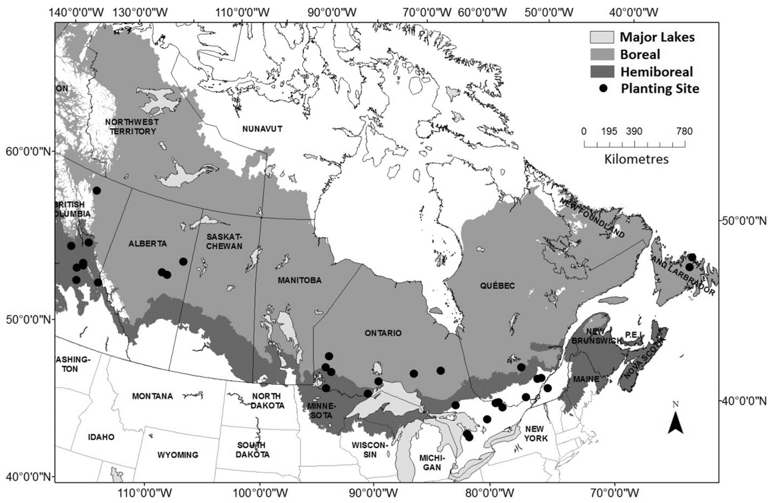
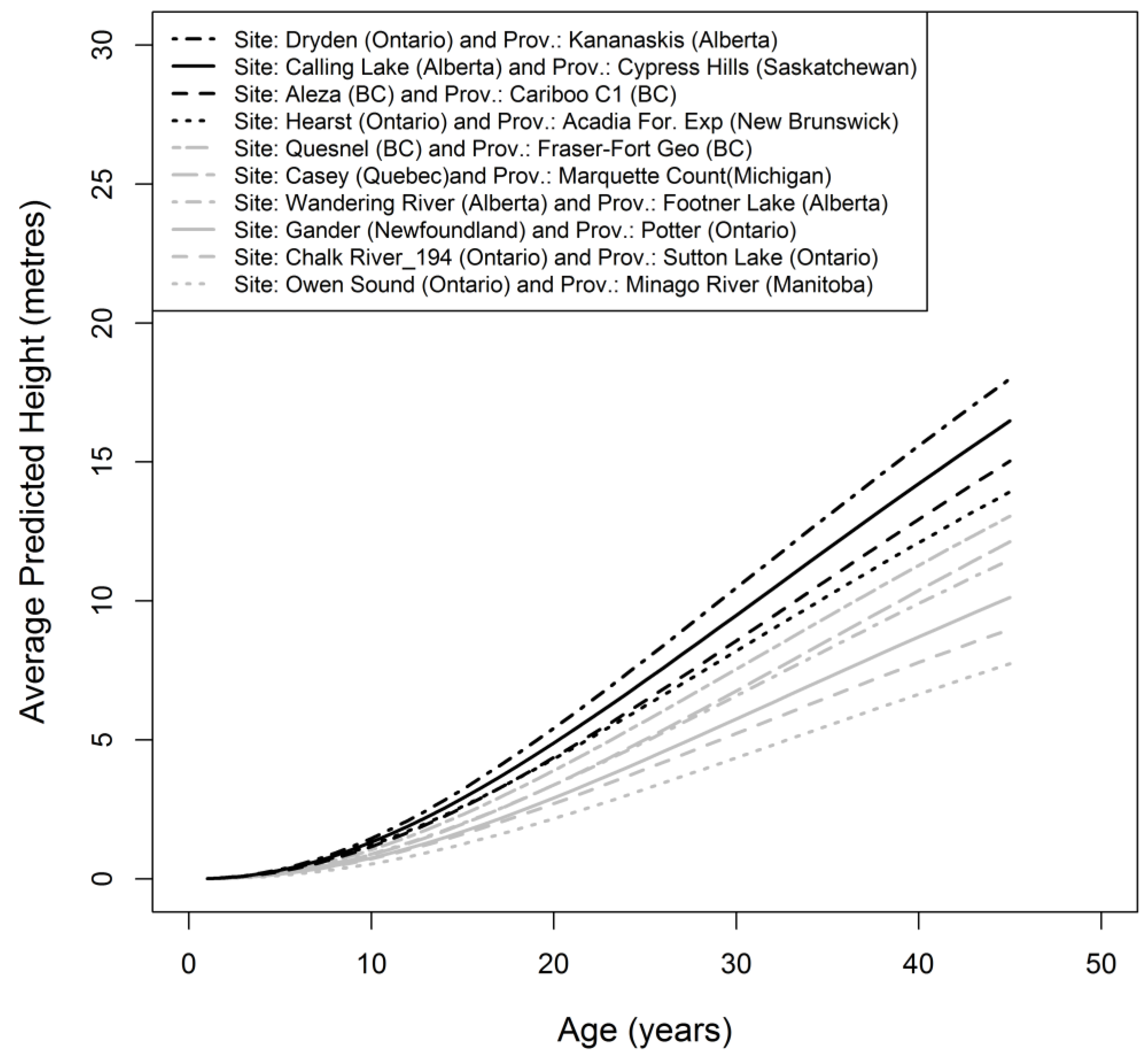
2.1. Meta-Data and Height Trajectories

The meta-data for this study were previously used in [31]. Briefly, the meta-data of 18 studies, representing 38 planting sites in Canada (Figure 1), with provenances from Canada and the United States, were collected from published articles, internal reports, government reports, and other sources, principally using the Web of Science^® (Science Citation Index Expanded) search engine, supplemented by additional data provided by authors in some cases.

Following the approach in [16], average heights were predicted from 1 to 45 years for each provenance at each planting site in the meta-data using the average height model developed by Ref. [31]:

$${\widehat{\mathrm{H}}}_{ijt}={\widehat{\theta }}_{1_{ij}}{\left(1-exp\left(1-{\widehat{\theta }}_{2_{ij}}{\mathrm{age}}_{ijt}\right)\right)}^{\left({\displaystyle \frac{1}{1-{\widehat{\theta }}_{3_{ij}}}}\right)}$$

(4)

$${\widehat{\theta }}_{1_{ij}}=30-0.00513 {\mathrm{s}\mathrm{i}\mathrm{t}\mathrm{e} \mathrm{e}\mathrm{l}\mathrm{e}\mathrm{v}\mathrm{a}\mathrm{t}\mathrm{i}\mathrm{o}\mathrm{n}}_i-0.1230\times {{\mathrm{D}\mathrm{M}\mathrm{A}\mathrm{T}}_{ij}}^2$$

$$-0.8768\times {\mathrm{D}\mathrm{M}\mathrm{A}\mathrm{T}}_{ij}+0.00796\times {\mathrm{p}\mathrm{r}\mathrm{o}\mathrm{v}\mathrm{e}\mathrm{n}\mathrm{a}\mathrm{n}\mathrm{c}\mathrm{e} \mathrm{e}\mathrm{l}\mathrm{e}\mathrm{v}\mathrm{a}\mathrm{t}\mathrm{i}\mathrm{o}\mathrm{n}}_j$$

(5)

$${\widehat{\theta }}_{2_{ij}}=0.0260+3.601\mathrm{E}-7\times {\mathrm{d}\mathrm{e}\mathrm{n}\mathrm{s}\mathrm{i}\mathrm{t}\mathrm{y}}_i+0.000020\times { \mathrm{D}\mathrm{D}\mathrm{d}\mathrm{i}\mathrm{f}}_{ij}$$

(6)

$${\widehat{\theta }}_{3_{ij}}=0.5674+0.000039\times {\mathrm{D}\mathrm{M}\mathrm{A}\mathrm{P}}_{ij}$$

(7)

where ${\widehat{\mathrm{H}}}_{ijt}$ is the predicted average height (m) of planting site i and provenance j measured at time t; age (years) is the plantation age; ${\widehat{\theta }}_{1_{ij}}$ is the estimated asymptote; ${\widehat{\theta }}_{2_{ij}}$ and ${\widehat{\theta }}_{3_{ij}}$ are shape parameters; site and provenance elevations are in meters; density is the planting density (stems per ha); and $\mathrm{D}\mathrm{M}\mathrm{A}\mathrm{T}$, DDdif, and DMAP are the distances for the mean annual daily temperature (MAT, °C), degree days > 5 °C (DDs, days), and mean annual precipitation (MAP, mm) between the planting site and provenance, respectively. These climatic distances were calculated for each provenance at each planting site, as described in [31], using climate normals for 1981–2010 from the Environment Canada database (https://climate.weather.gc.ca/, accessed on 10 September 2013) and from the National Oceanic and Atmospheric Administration’s (NOAA) National Climatic Data Center (NCDC) (https://www.cakex.org/community/directory/organizations/noaa-national-climatic-data-center-ncdc, accessed on 11 September 2013). A positive DMAT indicates that the planting site is warmer, a positive DMAP indicates that the planting site has higher precipitation, and a positive DDdif indicates that the planting site has more days with a mean temperature > 5 °C than the provenance location. The forecast was limited to age 45, since the oldest planting age at all study sites was 44. Using this approach, average height trajectories were obtained for the 38 planting sites, representing 337 provenances in the meta-data; some are illustrated in Figure 2. All graphs in this article were created using software R version 3.3.1 [32], except for Figure 1.

2.2. Effects of Age and Definition of Top Performers

Using the height trajectories from age 1 to 45 years, the relative height gain (RH) was calculated by planting site and age as follows:

$$\mathrm{G}\mathrm{a}\mathrm{i}\mathrm{n},\mathrm{RH}={\displaystyle \frac{\mathrm{a}\mathrm{v}\mathrm{e}\mathrm{r}\mathrm{a}\mathrm{g}\mathrm{e} \mathrm{h}\mathrm{e}\mathrm{i}\mathrm{g}\mathrm{h}\mathrm{t} \mathrm{o}\mathrm{f} \mathrm{t}\mathrm{o}\mathrm{p} \mathrm{x}\%-\mathrm{a}\mathrm{v}\mathrm{e}\mathrm{r}\mathrm{a}\mathrm{g}\mathrm{e} \mathrm{h}\mathrm{e}\mathrm{i}\mathrm{g}\mathrm{h}\mathrm{t} \mathrm{o}\mathrm{f} \mathrm{y}\%}{\mathrm{a}\mathrm{v}\mathrm{e}\mathrm{r}\mathrm{a}\mathrm{g}\mathrm{e} \mathrm{h}\mathrm{e}\mathrm{i}\mathrm{g}\mathrm{h}\mathrm{t} \mathrm{o}\mathrm{f} \mathrm{y}\%}}$$

(8)

where top x% is the percentile used to define the top performers selected at a particular evaluation age, and y% is the percentile used to define the baseline population. To illustrate this definition, Figure 3 shows 15% as the percentile for top performers based on an evaluation of 15 years relative to the baseline using all provenances (100%).

Changing the percentile used to define the top performers will also affect the gain. If the percentile is too low (e.g., top 5% or less), then the estimated gain would be unrealistically high, and the number of provenances switching in or out with different evaluation ages may be high. Conversely, if the percentile for top performers is too high, the estimated gain would be unrealistically low, but the evaluation age would likely have little impact, with few or no provenances switching in or out of the top performing group. Finally, the definition of the baseline also affects the gain. Two options are commonly used: 100% of all provenances in the trial or only the provenances excluded from the top performing group.

Four evaluation ages (5, 15, 25, and 45 years) were included in the sensitivity analysis, and the definition of the top performers was altered to reflect three different percentiles (5%, 15%, and 25%). Although the baseline was 100% for all of these combinations of evaluation ages and top performer definitions, it was also altered to be the bottom 75% percentile when coupled with the 25% top performers. Although these definitions generally cover the ranges found in the literature, the evaluation age was extended down to 5 years and up to 45 years. For each combination in this sensitivity analysis, the trend in gain over time was examined, along with how these trends changed with the gain definition. Based on this sensitivity analysis, as well as comparisons with other studies and experts’ opinions, one gain definition for the gain trajectory model was chosen.

Using the selected gain definition (i.e., an evaluation age of 15 years, the top 15%, and a 100% baseline), the relative height gain was calculated by planting site for ages 1 to 45 years as follows:

$$\mathrm{G}\mathrm{a}\mathrm{i}\mathrm{n},{\mathrm{R}\mathrm{H}}_{it}={\displaystyle \frac{\mathrm{a}\mathrm{v}\mathrm{e}\mathrm{r}\mathrm{a}\mathrm{g}\mathrm{e} \mathrm{h}\mathrm{e}\mathrm{i}\mathrm{g}\mathrm{h}\mathrm{t} \mathrm{o}\mathrm{f} \mathrm{t}\mathrm{o}\mathrm{p} 15\%-\mathrm{a}\mathrm{v}\mathrm{e}\mathrm{r}\mathrm{a}\mathrm{g}\mathrm{e} \mathrm{h}\mathrm{e}\mathrm{i}\mathrm{g}\mathrm{h}\mathrm{t} \mathrm{o}\mathrm{f} 100\%}{\mathrm{a}\mathrm{v}\mathrm{e}\mathrm{r}\mathrm{a}\mathrm{g}\mathrm{e} \mathrm{h}\mathrm{e}\mathrm{i}\mathrm{g}\mathrm{h}\mathrm{t} \mathrm{o}\mathrm{f} 100\%}}$$

(9)

2.3. Gain Trajectory Model

Using the chosen definition of gain, the gain was calculated for ages 1 to 45 for each of the 38 sites. Then, using an approach similar to that in [11], a flexible nonlinear gain model (i.e., a base model) was fitted:

$${\mathrm{RH}}_{it}={\beta }_0{\mathrm{age}}_{it}^{{\beta }_1}{\beta }_2^{{ \mathrm{age}}_{it}}+{ϵ}_{it}$$

(10)

where ${\mathrm{RH}}_{it}$ is the gain at planting site $i$ at measurement time $t$; ${\mathrm{age}}_{it}$ is the plantation age (years); ${\beta }_0$ is a scale parameter; ${\beta }_1$ and ${\beta }_2$ are shape parameters; and ${ϵ}_{it}$ is the error term. This base model represents the average gain trajectory over all planting sites. Other models were considered but were not selected since the functional form of this model better represents the relatively higher gains of very young plantations and the lower and nearly constant gain of later ages. Also, since this base model inherently includes a zero-intercept, the gain was restricted to be equal to 0 for a plantation age of 0. An intercept-only model (i.e., a null model) was also fitted. Because the meta-data for most planting sites included repeated measures with irregular intervals in plantation ages, first- and second-order continuous autoregressive parameters (CAR(x)) were added to the models. The models were then fitted using PROC MODEL of SAS software version 9.3 [33], which allows for autoregressive parameters. Several sets of starting parameters were used to ensure a global optimum solution for each model. Akaike’s information criterion (AIC) was calculated for the base and null models as follows:

$$\mathrm{A}\mathrm{I}\mathrm{C}=-2{log}_{e}L+2p$$

(11)

where $L$ is the maximum likelihood of the equation, and p is the number of parameters in the model. A large change in AIC relative to the null model was used as evidence that the gain changed with plantation age.

The base model was then altered using a random coefficients (also known as parameter prediction) modeling approach to examine whether the gains also differed with planting site characteristics. Specifically, the parameters in Equation (10) were allowed to vary by replacing them with the functions of planting site climatic variables and other site characteristics:

$${\mathrm{RH}}_{it}={\beta }_{0i}{\mathrm{age}}_{it}^{{\beta }_{1i}}{\beta }_{2i}^{{ \mathrm{age}}_{it}}+{ϵ}_{it}$$

(12)

$${\beta }_{0_i}=\mathrm{f}\left(\mathrm{site} {\mathrm{c}\mathrm{l}\mathrm{i}\mathrm{m}\mathrm{a}\mathrm{t}\mathrm{i}\mathrm{c}}_i,{\mathrm{o}\mathrm{t}\mathrm{h}\mathrm{e}\mathrm{r} \mathrm{s}\mathrm{i}\mathrm{t}\mathrm{e} \mathrm{c}\mathrm{h}\mathrm{a}\mathrm{r}\mathrm{a}\mathrm{c}\mathrm{t}\mathrm{e}\mathrm{r}\mathrm{i}\mathrm{s}\mathrm{t}\mathrm{i}\mathrm{c}\mathrm{s}}_i\right)+{\delta }_{0_i}$$

(13)

$${\beta }_{1_i}=\mathrm{f}\left(site {\mathrm{c}\mathrm{l}\mathrm{i}\mathrm{m}\mathrm{a}\mathrm{t}\mathrm{i}\mathrm{c}}_i,{\mathrm{o}\mathrm{t}\mathrm{h}\mathrm{e}\mathrm{r} \mathrm{c}\mathrm{h}\mathrm{a}\mathrm{r}\mathrm{a}\mathrm{c}\mathrm{t}\mathrm{e}\mathrm{r}\mathrm{i}\mathrm{s}\mathrm{t}\mathrm{i}\mathrm{c}\mathrm{s}}_i\right)+{\delta }_{1_i}$$

(14)

$${\beta }_{2_i}=\mathrm{f}\left(site {\mathrm{c}\mathrm{l}\mathrm{i}\mathrm{m}\mathrm{a}\mathrm{t}\mathrm{i}\mathrm{c}}_i,{\mathrm{o}\mathrm{t}\mathrm{h}\mathrm{e}\mathrm{r} \mathrm{c}\mathrm{h}\mathrm{a}\mathrm{r}\mathrm{a}\mathrm{c}\mathrm{t}\mathrm{e}\mathrm{r}\mathrm{i}\mathrm{s}\mathrm{t}\mathrm{i}\mathrm{c}\mathrm{s}}_i\right)+{\delta }_{2_i}$$

(15)

where ${RH}_{it}$, ${age}_{it}$, and ${ϵ}_{it}$ are as previously defined, and ${\delta }_{0_i}$, ${\delta }_{1_i}$, and ${\delta }_{2_i}$ are random effects at the site level. The submodels (Equations (13) to (15)) were fitted using combinations of predictor variables, specifically the planting site climatic variables (MAT, MAP, and DD), planting density, and planting site elevation. Again, all of these models were fitted using PROC MODEL of SAS software version 9.3 [33], which allows for continuous autoregressive parameters, and several sets of starting parameters were used to try to obtain a global optimum solution for each model fitted. Changes in AIC for these models relative to the base model were used to indicate whether site characteristics affected gain, after accounting for any changes due to plantation age. Changes in AIC were also used to evaluate alternative variable subsets. As a further indicator of model fit, the predicted gain trajectory for each possible model was superimposed on the measured gains for each planting site.

The baseline model was then fitted (Equation (10)), along with the null model. Then, several combinations of planting site climatic variables (the MAT, MAP, and DD) and other variables (e.g., planting density and site elevation) were used to model the scale and shape parameters (Equation (12), including (13) to (15)). A selection of these models based on improvements in AIC are listed in

Table 1. Fit statistics for a subset of height gain trajectory models.

Model	Parameter			AIC
	a Scale $({\widehat{\mathbf{\beta }}}_0)$	Shape 1 $({\widehat{\mathbf{\beta }}}_1)$	Shape 2 $({\widehat{\mathbf{\beta }}}_2)$
Null	Intercept only model			−8124
Base (I)	${\widehat{\mathsf{\beta }}}_0$	${\widehat{\mathsf{\beta }}}_1$	${\widehat{\mathsf{\beta }}}_2$	−8206
II	$b_{00}+b_{01}{\mathrm{M}\mathrm{A}\mathrm{P}}^2+b_{02} \mathrm{D}\mathrm{D}$	$b_{10}+b_{11}\mathrm{l}\mathrm{n}\left(\mathrm{d}\mathrm{e}\mathrm{n}\mathrm{s}\mathrm{i}\mathrm{t}\mathrm{y}\right)$	$b_{20}+b_{21}\mathrm{M}\mathrm{A}\mathrm{T}+b_{22}\mathrm{M}\mathrm{A}\mathrm{P}$	−15,298
III	$b_{00}+b_{01}{\mathrm{M}\mathrm{A}\mathrm{T}}^2+b_{02} \mathrm{s}\mathrm{i}\mathrm{t}\mathrm{e} \mathrm{e}\mathrm{l}\mathrm{e}\mathrm{v}\mathrm{a}\mathrm{t}\mathrm{i}\mathrm{o}\mathrm{n}$	$b_{10}+b_{11}\mathrm{l}\mathrm{n}\left(\mathrm{d}\mathrm{e}\mathrm{n}\mathrm{s}\mathrm{i}\mathrm{t}\mathrm{y}\right)$	$b_{20}+b_{21}\mathrm{M}\mathrm{A}\mathrm{T}+b_{22}\mathrm{M}\mathrm{A}\mathrm{P}$	−18,684
IV	$b_{00}+b_{01}{\mathrm{M}\mathrm{A}\mathrm{T}}^2+b_{02} \mathrm{s}\mathrm{i}\mathrm{t}\mathrm{e} \mathrm{e}\mathrm{l}\mathrm{e}\mathrm{v}\mathrm{a}\mathrm{t}\mathrm{i}\mathrm{o}\mathrm{n}$	$b_{10}+b_{11}\mathrm{l}\mathrm{n}\left(\mathrm{d}\mathrm{e}\mathrm{n}\mathrm{s}\mathrm{i}\mathrm{t}\mathrm{y}\right)$	$b_{20}+b_{21}\mathrm{M}\mathrm{A}\mathrm{T}$	−18,666
V	$b_{10}+b_{11}{\mathrm{M}\mathrm{A}\mathrm{P}}^2+b_{12} \mathrm{D}\mathrm{D}$	$b_{10}+b_{11}\mathrm{l}\mathrm{n}\left(\mathrm{d}\mathrm{e}\mathrm{n}\mathrm{s}\mathrm{i}\mathrm{t}\mathrm{y}\right)$	$b_{20}+b_{21}\mathrm{M}\mathrm{A}\mathrm{P}$	−15,244
VI	$b_{00}+b_{01}{\mathrm{M}\mathrm{A}\mathrm{T}}^2+b_{02 } \mathrm{s}\mathrm{i}\mathrm{t}\mathrm{e} \mathrm{e}\mathrm{l}\mathrm{e}\mathrm{v}\mathrm{a}\mathrm{t}\mathrm{i}\mathrm{o}\mathrm{n}$	$b_{10}+b_{11}\mathrm{l}\mathrm{n}\left(\mathrm{d}\mathrm{e}\mathrm{n}\mathrm{s}\mathrm{i}\mathrm{t}\mathrm{y}\right)$	$b_{20}+b_{21}\mathrm{D}\mathrm{D}$	−18,665
VII	$b_{00}+b_{01}{\mathrm{M}\mathrm{A}\mathrm{T}}^2+b_{02}{\mathrm{M}\mathrm{A}\mathrm{P}}^2+b_{03} \mathrm{D}\mathrm{D}+b_{04} \mathrm{s}\mathrm{i}\mathrm{t}\mathrm{e} \mathrm{e}\mathrm{l}\mathrm{e}\mathrm{v}\mathrm{a}\mathrm{t}\mathrm{i}\mathrm{o}\mathrm{n}$	$b_{10}+b_{11}\mathrm{l}\mathrm{n}\left(\mathrm{d}\mathrm{e}\mathrm{n}\mathrm{s}\mathrm{i}\mathrm{t}\mathrm{y}\right)$	$b_{20}+b_{21}\mathrm{M}\mathrm{A}\mathrm{T}+b_{22}\mathrm{M}\mathrm{A}\mathrm{P}$	−19,136

^a MAT (°C) is the mean annual daily temperature; DD (days) is the degree days greater than 5 °C; MAP (mm) is the mean annual precipitation; density is the planting density (stems ha⁻¹); and site elevation is in meters.

. As noted, first- and second-order continuous autoregressive parameters were added to the models, but the second-order continuous autoregressive parameter was not statistically significant (p-value > 0.05) for any model and was dropped.

Finally, one model was selected using the AIC values and the observed versus estimated gain graphs. For the selected model, validation statistics were calculated using the “leave-one-out” approach, where one planting site was excluded from model fitting, and the model was applied to the excluded planting site. This was repeated for each planting site, and the results were summarized into the root mean square predicted error (RMSPE):

$$\mathrm{R}\mathrm{M}\mathrm{S}\mathrm{P}\mathrm{E}=\sqrt{{\displaystyle \frac{\sum _{i=1}^n\sum _{t=1}^l{\left({\mathrm{R}\mathrm{H}}_{it}-{\widehat{\mathrm{R}\mathrm{H}}}_{it}\right)}^2}{T}}}$$

where $i=1, \dots , n$planting sites, $t=1, \dots , l$ measurement times within planting sites, ${\widehat{\mathrm{R}\mathrm{H}}}_{it}$is the predicted gain, and $T$ is the total number of observations.

3. Results

3.1. Gain Definition Sensitivity Analysis

The general trend of gain over time was nonlinear regardless of the evaluation age, as illustrated in Figure 4 for four planting sites using 15% for the top performers and 100% for the baseline. The gain trends were similar in shape among different planting sites, but the levels changed (e.g., Petawawa, Ontario vs. Calling Lake, Alberta).

The gain trajectory derived from the "changing performers" (top 15% selected at each age) showed two phases of similarity when compared to that derived from the fixed evaluation age. In the early phase (up to plantation age 15), it was comparable to that derived from a fixed evaluation at age 5. In the later phase (beyond age 15), it more closely resembled the trajectories derived from fixed evaluation ages of 15, 25, or 45 years. This indicates that the selected top performers at a particular evaluation age were not top performers at other ages. An evaluation age of 5 years was the most different from the “changing performers” trend, as might be expected. This is because the top performing provenances selected at evaluation age 15 years were quite similar to the “changing performers” and to evaluation ages 25 and 45; additionally, this evaluation age is easier to apply in practice. Although the interval between 25 and 45 years is long and encompasses a period of significant stand development, our results demonstrate that the gain trajectories derived from these later evaluation ages were very similar (Figure 4), indicating that the ranking of top performing provenances was stable during this period. Thus, we chose 15 years as the evaluation age to be used in the gain calculations used for the gain trajectory model.

Using a selected evaluation age of 15 years and the baseline as the average of all provenances (i.e., 100%), both the levels and the shapes of the gain trajectories changed with the definition of the top performers, as illustrated for four planting sites in Figure 5. The levels were similar when using the top 15% and 25% but quite different when using the top 5%. As shown by these four planting sites (Figure 5), the gain trends varied by planting site. Calling Lake had lower gains when using the top 15% and top 25% in particular. The shape generally became less curved when going from the top 25% to the top 5%, except for Aleza, BC, where the shape became concave when using the top 5%. Using the top 25% but varying the baseline from 100% to 75% (i.e., using only the excluded provenances) resulted in a perception of higher gains compared to using a baseline of 100% for that top percentage.

Overall, this sensitivity analysis indicated the importance of the definition used in calculating the gain. Using the top 15% perhaps provides a more realistic indicator of gain than using either 5% or 25%. In terms of the baseline, the use of 100% as the baseline is perhaps more common in the literature. Further, if the gain will be used to adjust an existing plantation growth and yield model, it can be argued that the existing model could represent the average of all provenances planted, and the 100% baseline would be more suitable. Thus, we chose to use the top 15% and 100% as the baselines in our gain trajectory model.

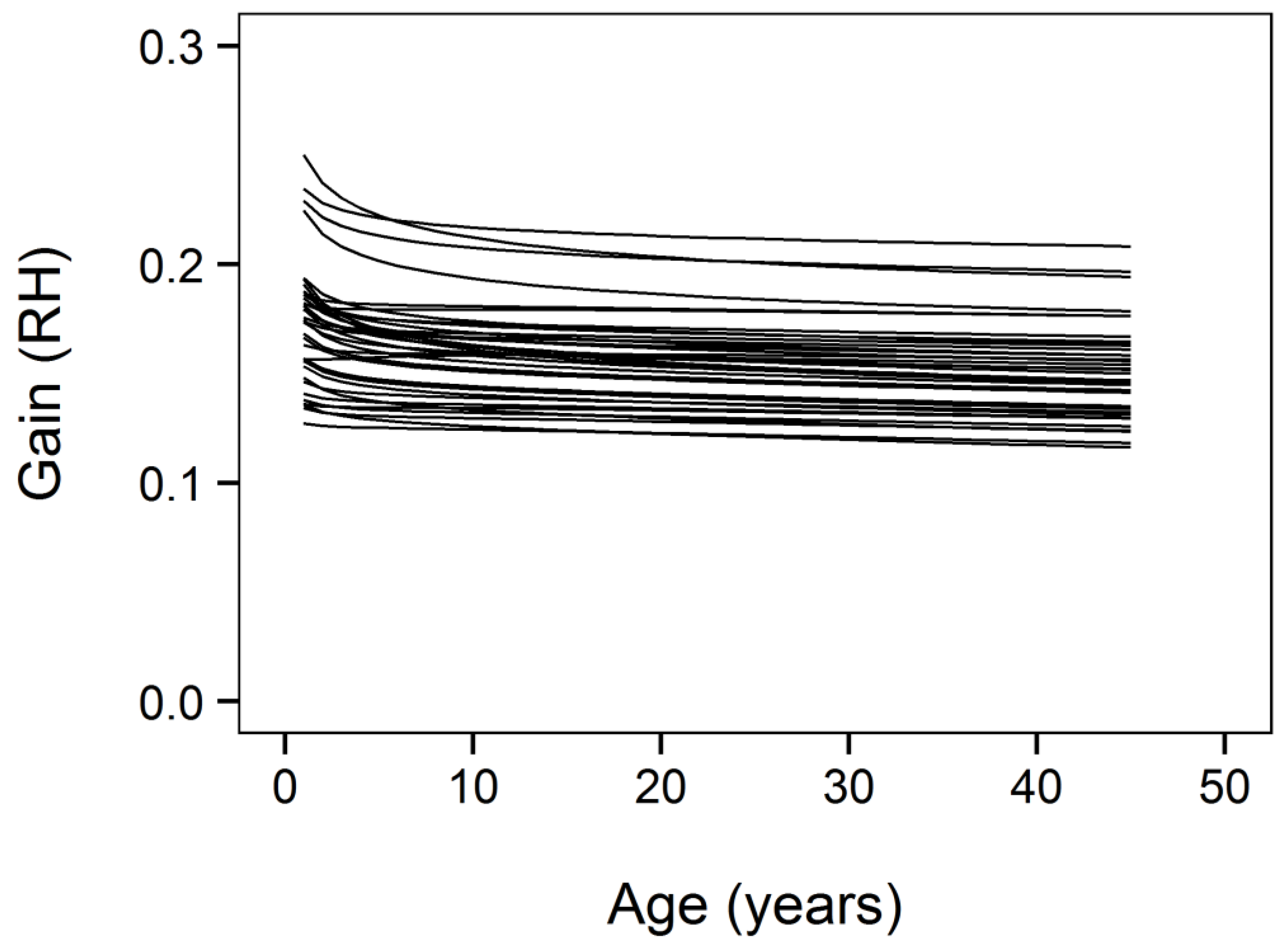
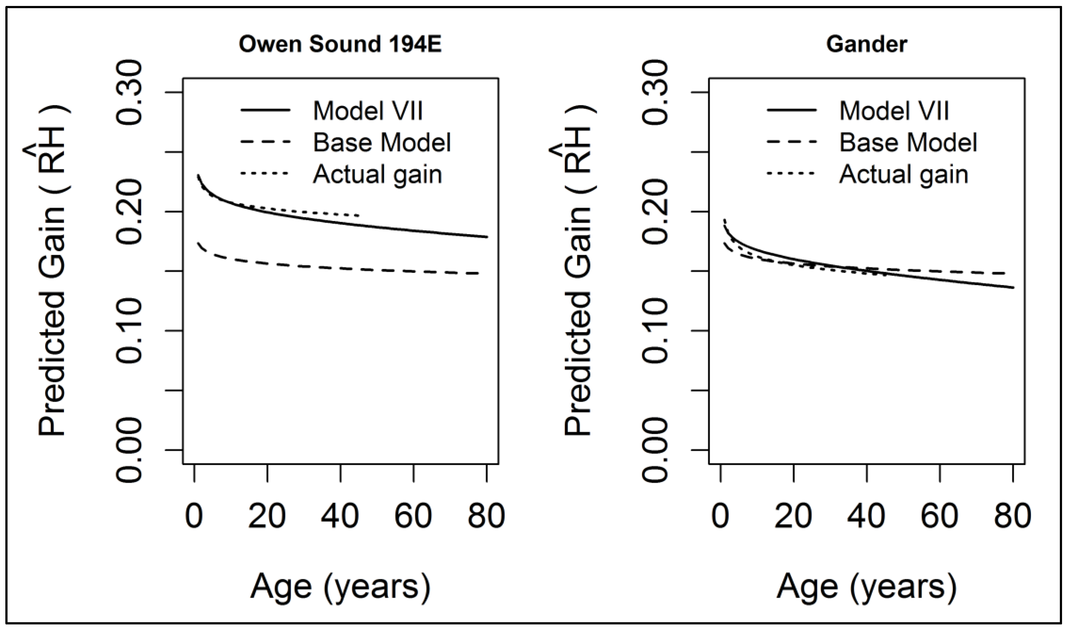
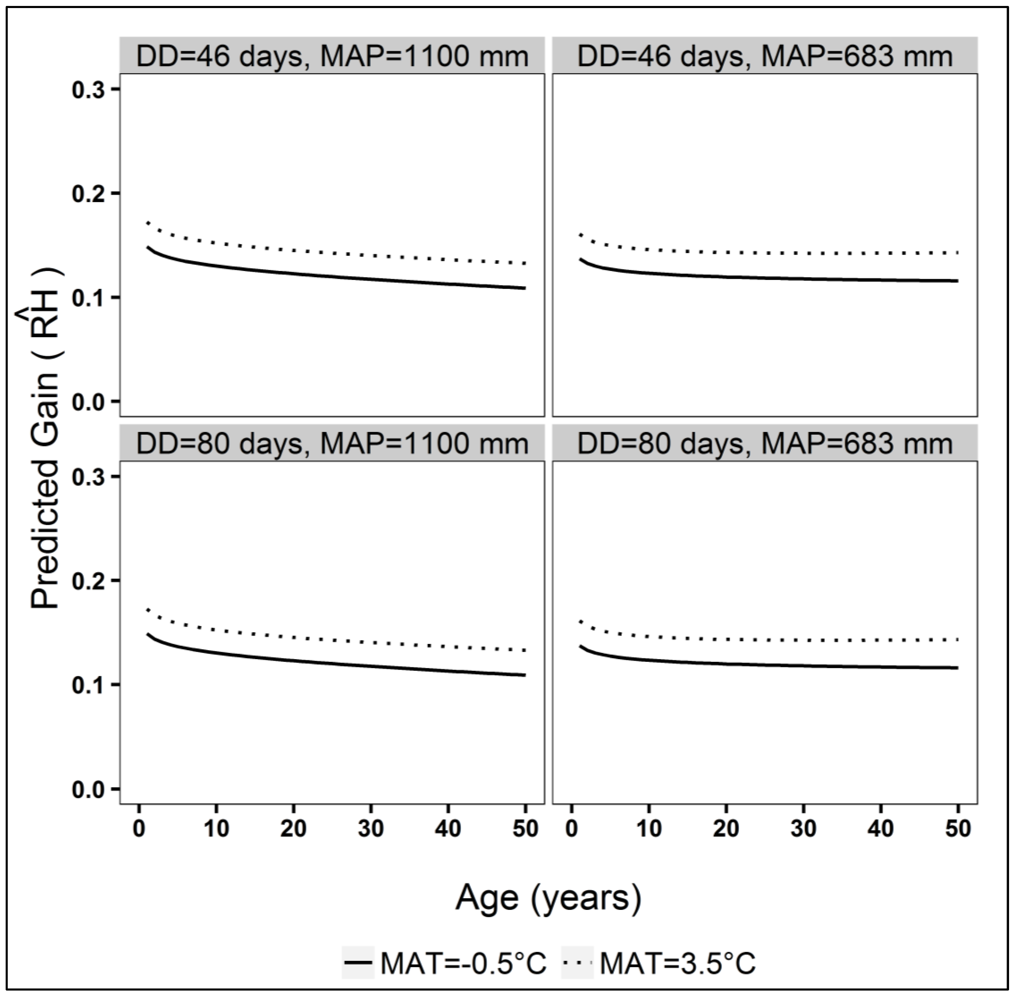
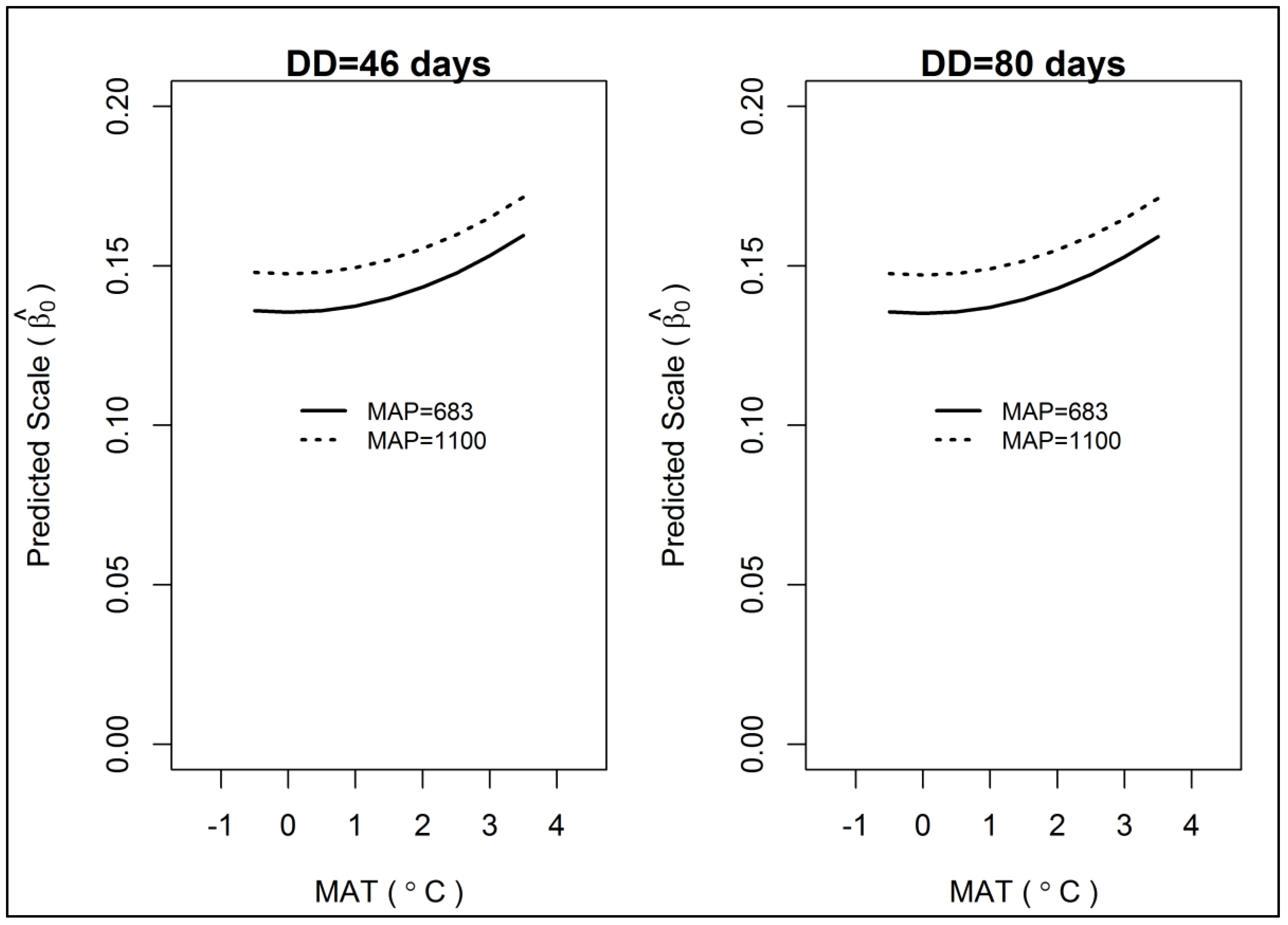
3.2. Gain Trajectory Model

The gain trajectories calculated using the selected gain definition are shown for all planting sites in Figure 6.

Table 1 shows the fit statistics for a selection of the height gain trajectory models that were tested.

The change in AIC for the null versus the base model (Model I) indicated that the height gain changed with plantation age (Table 1). To illustrate the differences in using a single multiplier versus allowing for changes with plantation age, the actual gains versus estimated gains using the null model (intercept = average gain = 0.157182) and using the base model (${\widehat{\beta }}_0=0.173562$, ${\widehat{\beta }}_1=-0.03347$, and ${\widehat{\beta }}_2=0.999845$) were graphed for two planting sites, “Owen Sound 194E” and “Gander”, both with a planting density of 3086 stems per ha (i.e., 1.8 m spacing) (Figure 7). For both sites, the base model reflected a drop in gain with plantation age, unlike the commonly used multiplier, which did not change with age, represented by the null model. However, for Gander, the base model also mimicked the gain levels by age, whereas these were underestimated by about 0.15 for Owen Sound 19E. These two sites illustrate the improvements obtained when allowing for changes in gain with plantation age, but they also illustrate that other site variables are needed to represent the actual gains by plantation age at the site level.

Further improvements in predicting height gain were obtained by allowing the parameters of the base model to change with the planting site characteristics (Models II to VII), as indicated by the AIC values being lower than those of the base model (Model I) (Table 1). The scale parameters estimated for each site (Equation (12)) showed a nonlinear trend with the MAT and MAP; as a result, ${\mathrm{M}\mathrm{A}\mathrm{T}}^2$ and ${\mathrm{M}\mathrm{A}\mathrm{P}}^2$ were included as possible predictor variables for submodel 8a. One or both of these variables were included in all models shown in Table 1. A nonlinear trend with planting density was also noted for the first shape parameter (Equation (14)). A number of transformations were evaluated, and the natural logarithm of planting density was the only predictor variable selected for this submodel. Only climate variables were included in the second shape parameter submodel (Equation (15)).

Model VII, which had the largest number of predictor variables, had the smallest AIC (−19,136), which was substantially lower than that of the base model (−8206). Further, Model VII had smaller AIC values than the other models (about 4000 less than Models II and V and about 400 less than Models III, IV, and VI). Additionally, the predicted height trajectories superimposed on the observed data showed the best fit for Model VII. As a result, Model VII was selected to estimate gains (

Table 2. Parameter estimates (and standard errors) for the selected gain trajectory model.

Equation (12) Parameter	Variable a	Parameter Estimate (Standard Error)
${\beta }_0$ (scale)	Intercept	0.12455 (0.000271)
	${\mathrm{MAT}}^2$ (°C)	0.0019668 $(5.395\times {10}^{-6}$ )
	${\mathrm{MAP}}^2$ (mm)	$1.6164\times {10}^{-8}$ $(1.94\times {10}^{-10}$ )
	DD (days)	−0.000011170 $(2.293\times {10}^{-6}$ )
	Site elevation (m)	9.6782 × 10−6 $(2.129\times {10}^{-7}$ )
${\beta }_{1_i}$ (shape 1)	Intercept	−0.051836 (0.00463)
	ln(density) (stems ha−1)	0.0010935 (0.000586)
${\beta }_{2_i}$ (shape 2)	Intercept	1.0053153 (0.000947)
	MAT (°C)	0.00025649 (0.000209)
	MAP (mm)	$-6.9969\times {10}^{-6}$ $(1.35\times {10}^{-6}$ )

^a MAT is the mean annual daily temperature (°C); DD (days) is the degree days greater than 5 °C; MAP (mm) is the mean annual precipitation (mm); density (stems ha⁻¹) is the planting density; and site elevation is in meters.

). The RMSPE for this model was found to be 0.0042 using the “leave-one-out” model validation procedure.

To illustrate the improvements obtained when using the predicted height gain trajectories allowing for changes due to planation age and site characteristics (Model VII) as opposed to those allowing for changes due to plantation age only (base model, Model I), the gain trajectories are again shown for the “Owen Sound 194E” and “Gander” planting sites (Figure 8). Generally, the shapes of Model VII were similar to those of the base model, whereas the scale differed, indicating the importance of allowing submodel 3.8a to vary with the site characteristics and site climate. Unlike the base model, Model VII also represents the levels of gain for both sites and for all other sites (not shown) due to including site level variables as predictor variables.

The predictor variables of Model VII interact with each other (e.g., elevation, the MAP, and the MAT), making it difficult to examine the effects of each predictor variable on the gain trajectory. However, combinations of these variables within the range of the meta-data were selected, and the resulting gain trajectories were graphed. For this purpose, the planting site elevation and planting density were set to 400 m and 2500 stems per ha, respectively, based on the means of these variables in the meta-data. Then, all combinations of two MAPs (683 and 1100 mm), two MATs (−0.5 and 3.5 °C), and two DDs (46 and 80 days) were input into Model VII, along with ages from 0 to 50 years (Figure 9). Although these values represent the ranges within the meta-data, they may not strictly reflect the multivariate relationships within the predictor variables.

Changes in the DDs from 46 to 80 days had little impact (a difference in gain of less than 0.005) on the height gain trajectory (Figure 9). Increasing the MAT from −0.5 to 3.5 °C resulted in an increase in gain of about 0.03 across the plantation ages. Noticeable changes in the shape occurred when the MAP changed from 683 to 1100 mm, with a steeper and more curved shape for the higher precipitation level. Other graphs allowing the planting density and site elevation to change by fixing climate variables indicated that an increase in planting density from 1000 stems per ha to 2500 stems per ha resulted in only a small increase in the estimated gain (<0.005) and only for older plantations. An increase in the site elevation from 279 m to 600 m resulted in an increase in gain of 0.003 for most plantation ages.

As noted earlier, the scale parameter was more affected by site climate and other characteristics than by the two shape parameters. Although it is not possible to completely interpret the scale parameter separately from the other two parameters, simulations were used to examine the effects of planting site climate on this parameter. For this purpose, the planting site elevation and planting density were kept constant at 400 m and 2500 stems per ha, respectively. Then, the DDs, MAT, and MAP were allowed to vary within the range of values in the meta-data (Figure 10). Slightly larger values were obtained for a DD value of 46 days. The scale parameter increased with increases in the MAT and MAP, indicating that sites with better growing conditions have higher height gain trajectories.

4. Discussion

Relative height gain has been used as a basis for estimating gains in yields resulting from superior provenances in Canada and elsewhere. In many research papers, a simple relative height gain multiplier is estimated using provenance trial data, thereby implicitly or explicitly assuming that this gain multiplier does not vary over plantation age or site characteristics [11,12,19,20,21,22,23,25]. This assumption may not hold, particularly over the large spatial extents of spruce plantations in Canada. Modern approaches in genomic selection aim to overcome these limitations by predicting breeding values based on genome-wide markers, potentially capturing complex genetic architectures and improving prediction accuracy across different ages and environments [4,5,7]. Meta-data were used to examine these assumptions by including plantation age and site characteristics as possible predictor variables in a model to estimate height gain. The use of meta-regression in this study, similar to approaches used to synthesize loblolly pine data [17], allowed for the examination of gain trajectories across diverse site conditions, challenging the assumption of invariant gain multipliers. For this purpose, height trajectories for each provenance at all planting sites in the meta-data were created using climatic information of the provenance and planting site locations and the model developed in [31]. Once these height trajectories were obtained, models of the actual height gain over plantation age and for different planting site characteristics were developed.

We needed to address two issues before these gains could be calculated: (i) the age at which to identify top performers and (ii) the percentiles to use to define the top performers and the baseline. To address these issues, sensitivity analyses were used to examine the impacts of various evaluation ages and top performers/baseline definitions. With regards to the first issue, the sensitivity analyses showed that the choice of evaluation age resulted in different gain trajectories, but mostly when comparing an evaluation age of 5 years (plantation age) to older ages. Given that there was little change between using 15 and 45 years as evaluation ages and that earlier identification of improved stock is useful in practice, we chose an evaluation age of 15 years. Previous work supports this and other values. Ref. [34] suggested using an evaluation age at one-quarter of the harvest age for Douglas-fir to predict gain. Applying this to white spruce and given a harvest age of approximately 60–80 years for plantations, the recommended evaluation age would be 15 to 20 years, similar to that selected in this study. Ref. [10] used age 20 as the evaluation age for black spruce and jack pine to estimate gains in height, volume, and diameter and found that height gain declined sharply until age 20. Conversely, Ref. [9] used 50 years as the evaluation age to estimate the relative height gain of black spruce, jack pine, white spruce, and red pine. In Ref. [9] the choice of 50 years would be closer to the biological rotation ages of these species, but this may not be practical in application and may not be necessary based on the sensitivity analysis presented in this paper. Ref. [11] used data from seven white spruce progeny trials covering plantation ages of 13 to 22 years, depending on the trial, to estimate gain in dominant height.

With respect to the second issue, the definitions of top performers and the baseline affected both the gain trajectory level and the shape. The average of the top 15% of provenances was selected to define the top performers, and the average of all provenances (i.e., 100%) was selected as the baseline to estimate the gain of each planting site and plantation age. The values used to identify top performers and baselines vary across other studies, often without specific justification for the values used. Ref. [2] used 100% for the baseline, as did [16]. Ref. [9] used the top 25% relative to the remaining stock (i.e., 75%). Ref. [10] also used the top 25% of improved stock but used 100% of unimproved stock as the baseline. In some studies, top performers were based on “plus-trees” selected based on larger heights and diameters outside bark at breast height (i.e., DBHs measured at 1.3 m above ground) rather than on a particular percentile [35,36].

Using the selected definition, we found that the estimated height gain was 0.12 to 0.25 (i.e., 12 to 25%) for young plantations and 0.12 to 0.22 for 45-year-old plantations depending on the planting site. These values are similar to those found in other studies, although, as noted, the gain definition differs among studies. Ref. [9] estimated the height gain as 0.1240 (i.e., 12.40%) at age 50 years. Ref. [10] reported that the first-generation black spruce gain in height was 0.12 at age 20 and then projected the gain to be 0.07 to 0.08 by age 40 years.

Changes in height gain were found with plantation age, indicating that this is not invariant over age for white spruce. Ref. [20] also found changes in height gain over plantation age for radiata pine; the gain decreased from age 15 to age 45 years. Similarly, Ref. [10] noted a downward trend with age for black spruce. A number of other studies found differences in gain with plantation age, but simple gain multipliers were still used for simplicity [11,18,25]. Conversely, Ref. [9] found that gain was relatively constant over time in his meta-analysis of white spruce. However, he used the top 25% versus 75%, as noted earlier, which does not appear to vary greatly with age based on the sensitivity analysis in this study.

The height gain of white spruce also varied with planting site characteristics. This does not agree with the meta-analysis of white spruce reported in [9], which found no differences in gain among planting sites. However, a more extensive meta-dataset was used than that used in [9], covering a wider range of planting sites across a broad spatial extent, including sites in Alberta and the hemiboreal forests of British Columbia. In particular, the height gain trajectories varied with site climatic variables, specifically the MAT, MAP, and DDs, along with site elevation and planting density. Generally, height gains were larger for warmer sites (i.e., higher MAT) with more precipitation (i.e., higher MAP). This result is supported by evidence in the genetics literature on environment interactions [37,38,39,40,41]. Also, Ref. [22] found that gains in volume, diameter, and height increased in Douglas-fir stands at higher-productivity sites. Similarly, others (e.g., Ref. [19]) (for loblolly pine) found that genetic gains increased with the site index. Although planting density was included in the final model, the effects on gain were small relative to those of other site variables. Dominant height growth in even-aged stands is relatively unaffected by density [42]. Ref. [22] studied Douglas-fir plantations and found that the predicted height growth for improved stock was generally unaffected by the initial planting density. While provenance trials provide foundational information, integrating findings from studies with genomic approaches, such as genomic selection, could offer a more powerful strategy for future tree improvement efforts, potentially allowing for earlier selection and more precise targeting of complex traits like climate resilience [4,5,7].

Although this research contributes to the understanding of the impacts of the gain definition on the reported gains and trends in gain with time and examined the changes over plantation age and over planting densities, a number of difficulties in conducting this work should be noted. First, the so-called actual gain trajectories for each provenance at every site were based on height trajectories produced via a previously fitted model using the data in [31], as used in other studies (e.g., Ref. [16]). This allowed for both the extensive spatial range represented in the meta-data and the longer temporal range that was represented in only a portion of the meta-data. However, using the model-based height to age 45 trajectories could have introduced biases in the so-called actual gains. Further, the gains were based on the percentiles of provenances included in each provenance trial. As noted in [43,44], the selection of which provenances to include in each provenance trial affects the calculation of gain. Finally, although a very broad spatial coverage was included in the meta-data, there were still spatial gaps. However, these missing locations may not be suitable for white spruce plantations because of site characteristics (e.g., poor soil) or because they may be too far from mills and other facilities that might make use of these plantations. Furthermore, while the model accounted for climatic variables and site elevation, detailed soil property data were not consistently available across the wide range of historical studies included in our meta-data. Soil characteristics undoubtedly influence tree growth, and the inability to include them is a limitation of this study. Future research incorporating standardized soil data could help refine gain predictions and better explain site-level variation.

5. Conclusions

Based on a comprehensive sensitivity analysis, along with comparisons to other studies and experts’ opinions, one definition of potential gain was chosen. In particular, the top 15% of all provenances relative to all provenances evaluated at 15 years since planting was recommended. This could be applied across the boreal and hemiboreal forests of Canada, thereby facilitating comparisons and the aggregation of information. Using this definition, it was found that the height gains of white and hybrid spruces varied with plantation age and planting site characteristics. Consequently, the commonly used approach of a single gain multiplier for all ages and planting site characteristics may not reflect the gain trajectories. As an alternative, a height gain trajectory model was developed using a random coefficients (also known as parameter prediction) modeling approach to model the changes over time under varying site characteristics. The developed gain trajectory model provided accurate gain estimates for each planting site using site climate, planting density, and elevation as predictor variables. The reliability of this model for predictive purposes was confirmed through a rigorous leave-one-out cross-validation procedure, supporting its application for forecasting gain up to harvest age across Canadian boreal and hemiboreal forests. Although this was largely affected by the mean annual daily temperature of planting sites, it was also affected by the mean annual precipitation and degree days > 5 °C and, to a lesser degree, by planting density. The developed height gain model could be incorporated into an existing growth and yield model to forecast potential gains in crop yields over time. Overall, this model shows potential for improving yields based on tree improvement programs in the boreal and hemiboreal forests of Canada.

References

1. Fins, L.; Friedman, S.T.; Brotschol, J.V. Handbook of Quantitative Forest Genetics; Kluwer Academic Publishers: Dordrecht, The Netherlands, 1992; 403p. [Google Scholar]
2. Zobel, B.; Talbert, J. Applied Forest Tree Improvement; J. Wiley & Sons: New York, NY, USA, 1984; 505p. [Google Scholar]
3. White, T.L.; Adams, W.T.; Neale, D.B. Forest Genetics; CABI Publishing: Cambridge, MA, USA, 2007. [Google Scholar]
4. Grattapaglia, D. Twelve Years into Genomic Selection in Forest Trees: Climbing the Slope of Enlightenment of Marker Assisted Tree Breeding. Forests 2022, 13, 1554. [Google Scholar] [CrossRef]
5. Lebedev, V.G.; Lebedeva, T.N.; Shestibratov, K.A. Genomic Selection for Forest Tree Improvement: Methods, Achievements and Perspectives. Forests 2020, 11, 1190. [Google Scholar] [CrossRef]
6. Cappa, E.P.; Chen, C.; Klutsch, J.G.; Sebastian-Azcona, J.; Ratcliffe, B.; Wei, X.; Da Ros, L.; Liu, Y.; Bhumireddy, S.R.; Benowicz, A.; et al. Revealing stable SNPs and genomic prediction insights across environments enhance breeding strategies of productivity, defense, and climate-adaptability traits in white spruce. Heredity 2025, 134, 186–199. [Google Scholar] [CrossRef]
7. Cappa, E.P.; Klutsch, J.G.; Sebastian-Azcona, J.; Ratcliffe, B.; Wei, X.; Da Ros, L.; Liu, Y.; Chen, C.; Benowicz, A.; Sadoway, S.; et al. Integrating genomic information and productivity and climate-adaptability traits into a regional white spruce breeding program. PLoS ONE 2022, 17, e0264549. [Google Scholar] [CrossRef] [PubMed]
8. Xiang, B.; Chen, Z.-Q.; Chen, J. Integrating evolutionary genomics of forest trees to inform future tree breeding amid rapid climate change. Plant Commun. 2024, 5, 100890. [Google Scholar] [CrossRef]
9. Newton, P.F. Systematic review of yield responses of four North American conifers to forest tree improvement practices. For. Ecol. Manag. 2003, 172, 29–51. [Google Scholar] [CrossRef]
10. McInnis, B.; Tosh, K. Genetic gains from 20 years of cooperative tree improvement in New Brunswick. For. Chron. 2004, 80, 127–133. [Google Scholar] [CrossRef]
11. Petrinovic, J.F.; Gélinas, N.; Beaulieu, J. Benefits of using genetically improved white spruce in Quebec: The forest landowner’s viewpoint. For. Chron. 2009, 85, 571–580. Available online: http://pubs.cif-ifc.org/doi/pdf/10.5558/tfc85571-4 (accessed on 15 April 2017). [CrossRef]
12. Nance, W.L.; Wells, O.O. Site index for models for height growth of planted loblolly pine (Pinus taeda L.) seed sources. In Proceedings of the 16th Southern Forest Tree Improvement Conference, Blacksburg, VA, USA, 27–28 May 1981; pp. 86–96. [Google Scholar]
13. Hamilton, D.A.; Rehfeldt, G.E. Using individual tree growth projection models to estimate stand-level gains attributable to genetically improved stock. For. Ecol. Manag. 1994, 68, 189–207. [Google Scholar] [CrossRef]
14. Stage, A.R. Prognosis Model for Stand Development; USDA Forest Service General Technical Report. INT-137; Intermountain Forest and Range Experiment Station: Ogden, UT, USA, 1973. [Google Scholar]
15. Wykoff, W.; Crookston, N.L.; Stage, A.R. User’s Guide to the Stand Prognosis Model; USDA Forest Service General Technical Report. INT-133; Intermountain Forest and Range Experiment Station: Ogden, UT, USA, 1982. [Google Scholar]
16. Magnussen, S.; Yanchuk, A.D. Time trends of predicted breeding values in selected crosses of coastal Douglas-fir in British Columbia: A methodological study. For. Sci. 1994, 40, 663–685. Available online: https://ostrnrcan-dostrncan.canada.ca/entities/publication/cd9de0c8-56a2-4683-90f0-eac7e3d283df (accessed on 15 April 2017). [CrossRef]
17. Restrepo, H.I.; Bullock, B.P.; Montes, C.R. Growth and yield drivers of loblolly pine in the southeastern U.S.: A meta-analysis. For. Ecol. Manag. 2019, 435, 205–218. [Google Scholar] [CrossRef]
18. Ahtikoski, A.; Ojansuu, R.; Haapanen, M.; Hynynen, J.; Kärkkäinen, K. Financial performance of using genetically improved regeneration material of Scots pine (Pinus sylvestris L.) in Finland. New For. 2012, 43, 335–348. [Google Scholar] [CrossRef]
19. Buford, M.A.; Burkhart, H.E. Genetic improvement effects on growth and yield of loblolly pine plantations. For. Sci. 1987, 33, 707–724. Available online: https://research.fs.usda.gov/treesearch/59531 (accessed on 13 April 2017). [CrossRef]
20. Carson, S.D.; Garcia, O.; Hayes, J.D. Realized gain and prediction of yield with genetically improved Pinus radiata in New Zealand. For. Sci. 1999, 45, 186–200. Available online: https://academic.oup.com/forestscience/article-abstract/45/2/186/4627556?redirectedFrom=fulltext&login=false (accessed on 13 April 2017). [CrossRef]
21. Adams, J.P.; Matney, T.G.; Land, S.B.; Belli, K.L.; Duzan, H.W. Incorporating genetic parameters into loblolly pine growth-and-yield model. Can. J. For. Res. 2006, 36, 1959–1967. [Google Scholar] [CrossRef]
22. Gould, P.; Johnson, R.; Marshall, D.; Johnson, G. Estimation of genetic-gain multipliers for modeling Douglas-fir height and diameter growth. For. Sci. 2008, 54, 588–596. Available online: https://www.fs.usda.gov/pnw/pubs/journals/pnw_2008_gould002.pdf (accessed on 13 April 2017). [CrossRef]
23. Lu, P.; Charrette, P. Genetic parameter estimates for growth traits of black spruce in northwestern Ontario. Can. J. For. Res. 2008, 38, 2994–3001. [Google Scholar] [CrossRef]
24. Gould, P.; Marshall, D. Incorporation of genetic gain into growth projections of Douglas-fir using ORGANON and the forest vegetation simulator. West. J. Appl. For. 2010, 25, 55–61. Available online: https://research.fs.usda.gov/treesearch/37821 (accessed on 13 April 2017). [CrossRef]
25. Ahtikoski, A.; Salminen, H.; Ojansuu, R.; Hynynen, J.; Kärkkäinen, K.; Haapanen, M. Optimizing stand management involving the effect of genetic gain: Preliminary results for Scots pine in Finland. Can. J. For. Res. 2013, 43, 299–305. [Google Scholar] [CrossRef]
26. Lambeth, C.C. Juvenile-mature correlations in Pinaceae and implications for early selection. For. Sci. 1980, 26, 571–580. [Google Scholar]
27. Lambeth, C.; Dill, L.A. Prediction models for juvenile-mature correlations for loblolly pine growth traits within, between and across test sites. For. Genet. 2001, 8, 101–108. [Google Scholar]
28. Di Lucca, C.M. TASS/SYLVER/TIPSY: Systems for predicting the impact of silvicultural practices on yield, lumber value, economic return and other benefits. In Stand Density Management Conference: Using the Planning Tools; Bamsey, C.R., Ed.; Clear Lake Ltd.: Edmonton, AB, Canada, 1999; pp. 7–16. [Google Scholar]
29. Xie, C.Y.; Yanchuk, A.D. Breeding values of parental trees, genetic worth of seed orchard seedlots, and yields of improved stocks in British Columbia. West. J. Appl. For. 2003, 18, 88–100. Available online: https://academic.oup.com/wjaf/article-abstract/18/2/88/4717963 (accessed on 15 April 2017). [CrossRef]
30. Alberta Tree Improvement and Seed Centre. Genetic Test Analysis Report for Region E. White Spruce Tree Improvement 15 Year Results; Technical report ATISC #10-28; Alberta Tree Improvement and Seed Centre: Smoky Lake, AB, Canada, 2011. [Google Scholar]
31. Ahmed, S.S. Impacts of Tree Improvement Programs on Yields of White Spruce and Hybrid Spruce in the Canadian Boreal Forest. Ph.D. Thesis, The University of British Columbia, Vancouver, BC, Canada, 2016. [Google Scholar]
32. R Core Team. R: A Language and Environment for Statistical Computing; R Foundation for Statistical Computing: Vienna, Austria, 2016; Available online: http://www.R-project.org/ (accessed on 15 April 2017).
33. SAS Institute Inc. SAS/STAT 13.2 User’s Guide; SAS Institute Inc.: Cary, NC, USA, 2014; 673p. [Google Scholar]
34. Johnson, R. Introduction to Forest Genetics. In Proceedings of the Genetics and Growth Workshop, Vancouver, WA, USA, 4−6 November 2003; pp. 20–39. [Google Scholar]
35. Xie, C.Y.; Yanchuk, A.D.; Kiss, G.K. Genetics of Interior Spruce in British Columbia: Performance and Variability of Open-Pollinated Families in the East Kootenays; Report no. 07; British Columbia Ministry of Forests Research Program: Victoria, BC, Canada, 1998. [Google Scholar]
36. Xie, C.Y. Genotype by environment interaction and its implications for genetic improvement of interior spruce in British Columbia. Can. J. For. Res. 2003, 33, 1635–1643. [Google Scholar] [CrossRef]
37. Morgenstern, M. Geographic Variation in Forest Trees: Genetic Basis and Application of Knowledge in Silviculture; UBC Press: Vancouver, BC, Canada, 1996; 224p. [Google Scholar]
38. Alberta Tree Improvement and Seed Centre. Genetic Test Analysis Report for Region E White Spruce Tree Improvement; Technical Report ATISC #04-22; Alberta Tree Improvement and Seed Centre: Smoky Lake, AB, Canada, 2004. [Google Scholar]
39. Rweyongeza, D.M.; Yang, R.C.; Dhir, N.K.; Barnhardt, L.K.; Hansen, C. Genetic variation and climatic impacts on survival and growth of white spruce in Alberta, Canada. Silvae Genet. 2007, 56, 117–126. Available online: https://ualberta.scholaris.ca/server/api/core/bitstreams/ee1761c2-2237-4a96-8d76-ae14137a66cc/content (accessed on 15 April 2017). [CrossRef]
40. Alberta Tree Improvement and Seed Centre. Controlled Parentage Program Plan for the Region G2 White Spruce Tree Improvement Project in the Northwest Boreal Region in Alberta; Technical Report ATISC #07-09; Alberta Tree Improvement and Seed Centre: Smoky Lake, AB, Canada, 2007. [Google Scholar]
41. Rweyongeza, D.M.; Barnhardt, L.K.; Hansen, C.R. Patterns of Optimal Growth for White Spruce Provenances in Alberta; Pub. No: Ref. T/255; Alberta Tree Improvement and Seed Centre: Smoky Lake, AB, Canada, 2011. [Google Scholar]
42. Pienaar, L.V.; Shiver, B.D. The effect of planting density on dominant height in unthinned slash pine plantations. For. Sci. 1984, 30, 1059–1066. Available online: https://academic.oup.com/forestscience/article/30/4/1059/4656945 (accessed on 15 April 2017).
43. Wright, J. Introduction to Forest Genetics; Academic Press: New York, NY, USA, 1976; 463p. [Google Scholar]
44. Namkoong, G. Introduction to Quantitative Genetics in Forestry; Technical Bulletin no. 1588; Forest Service, United States Department of Agriculture: Washington, DC, USA, 1979. [Google Scholar]
Figure 1. Geographic locations of planting sites in the meta-dataset.
Forests 16 01123 g001
Figure 2. Predicted average height trajectory of some white spruce provenances (Prov.) and planting sites (Site) in the meta-data.
Forests 16 01123 g002
Figure 3. Hypothetical predicted average height trajectory of white spruce populations showing top performing provenances (top 15%) versus all provenances (baseline 100%) at an evaluation age of 15 years.
Forests 16 01123 g003
Figure 4. Gain over time for four planting sites, where the top performers (15%) were selected at various evaluation ages (baseline is 100% of provenances). Gain based on selection of top performers at each age (“changing performers”) is included for comparison.
Forests 16 01123 g004
Figure 5. Gain over time at evaluation age 15 for different definitions of top performers (i.e., top 5%, 15%, or 25%) and baseline (i.e., 75% or 100%).
Forests 16 01123 g005
Figure 6. Gain over time by planting site.
Forests 16 01123 g006
Figure 7. Predicted height gains ( R H ^ ) over age using the null model and using the base model that changes with plantation age versus the actual gains for two planting sites.
Forests 16 01123 g007
Figure 8. Predicted height gain ( R H ^ ) over age for two planting sites using (i) Model VII; (ii) base model; and (iii) actual gain.
Forests 16 01123 g008
Figure 9. Changes in the predicted height gain ( R H ^ ) over age for combinations of values for site degree days (DDs), the mean annual daily temperature (MAT), and the mean annual precipitation (MAP), given a planting site elevation of 400 m and a planting density of 2500 stems per ha.
Forests 16 01123 g009
Figure 10. Changes in the estimated scale parameter ( β ^ 0 i ) with changes in site degree days (DDs), the mean annual daily temperature (MAT), and the mean annual precipitation (MAP), given a planting site elevation of 400 m and a planting density of 2500 stems per ha.
Forests 16 01123 g010