
Vegetation Growth Carryover and Lagged Climatic Effect at Different Scales: From Tree Rings to the Early Xylem Growth Season

 , ,
, ,
Abstract
1. Introduction
- (i)
- Investigate how the vegetation growth carryover (VGC) under two scales of tree-ring width (TRW) and the early xylem growth season (EXGs) can enhance signal acquisition and how it affects the growth in the next stage.
- (ii)
- Explore the persistence status of lagged climatic effects (LCE) on wood growth under the two scales of tree-ring width (TRW) and the early xylem growth season (EXGs).
- (iii)
- Assess the contribution rates of the wood growth persistence effect and the climate lag effect to vegetation growth under the two scales of tree-ring width (TRW) and the early xylem growth season (EXGs).
2. Materials
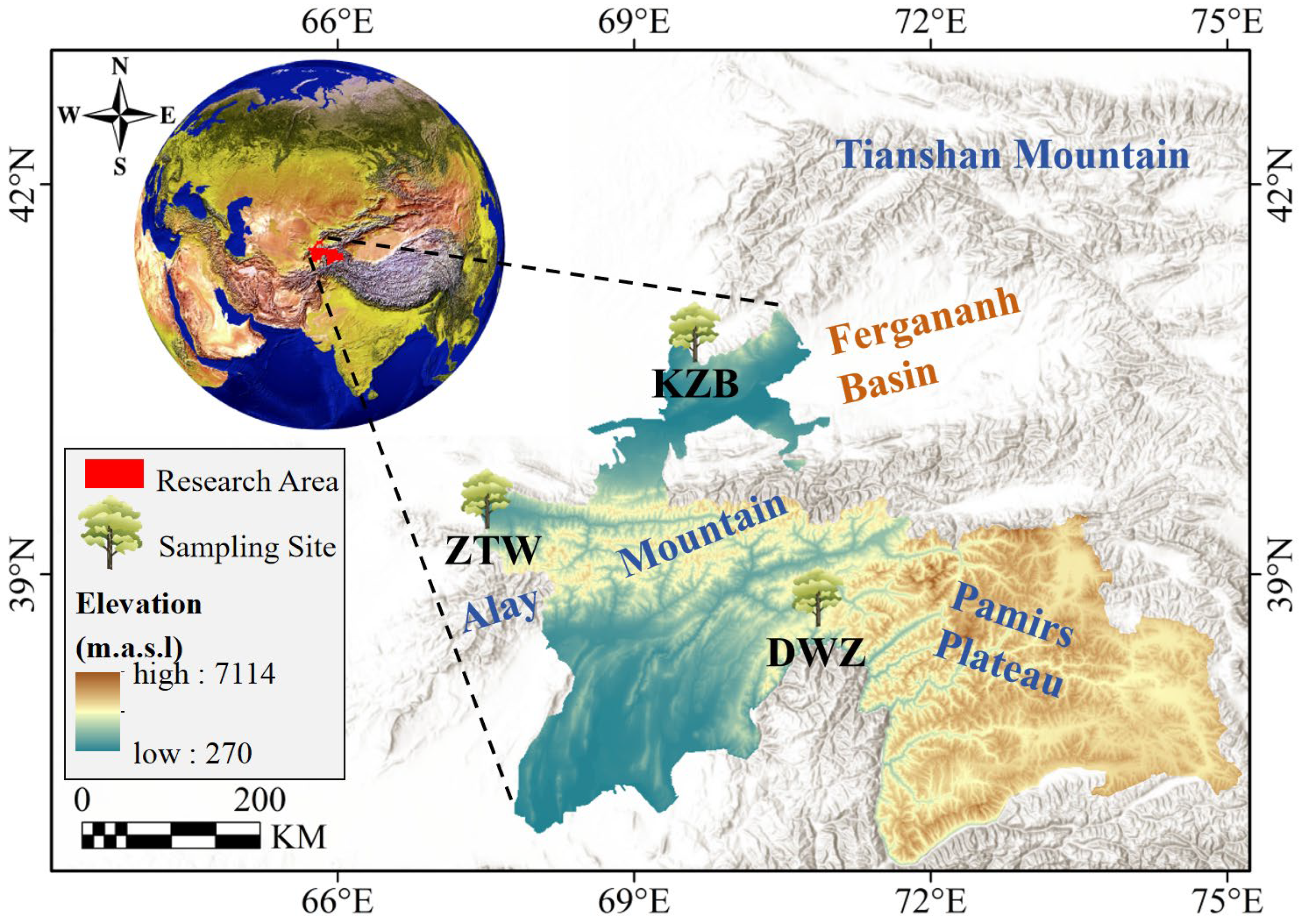
2.1. Study Site
2.2. Datasets
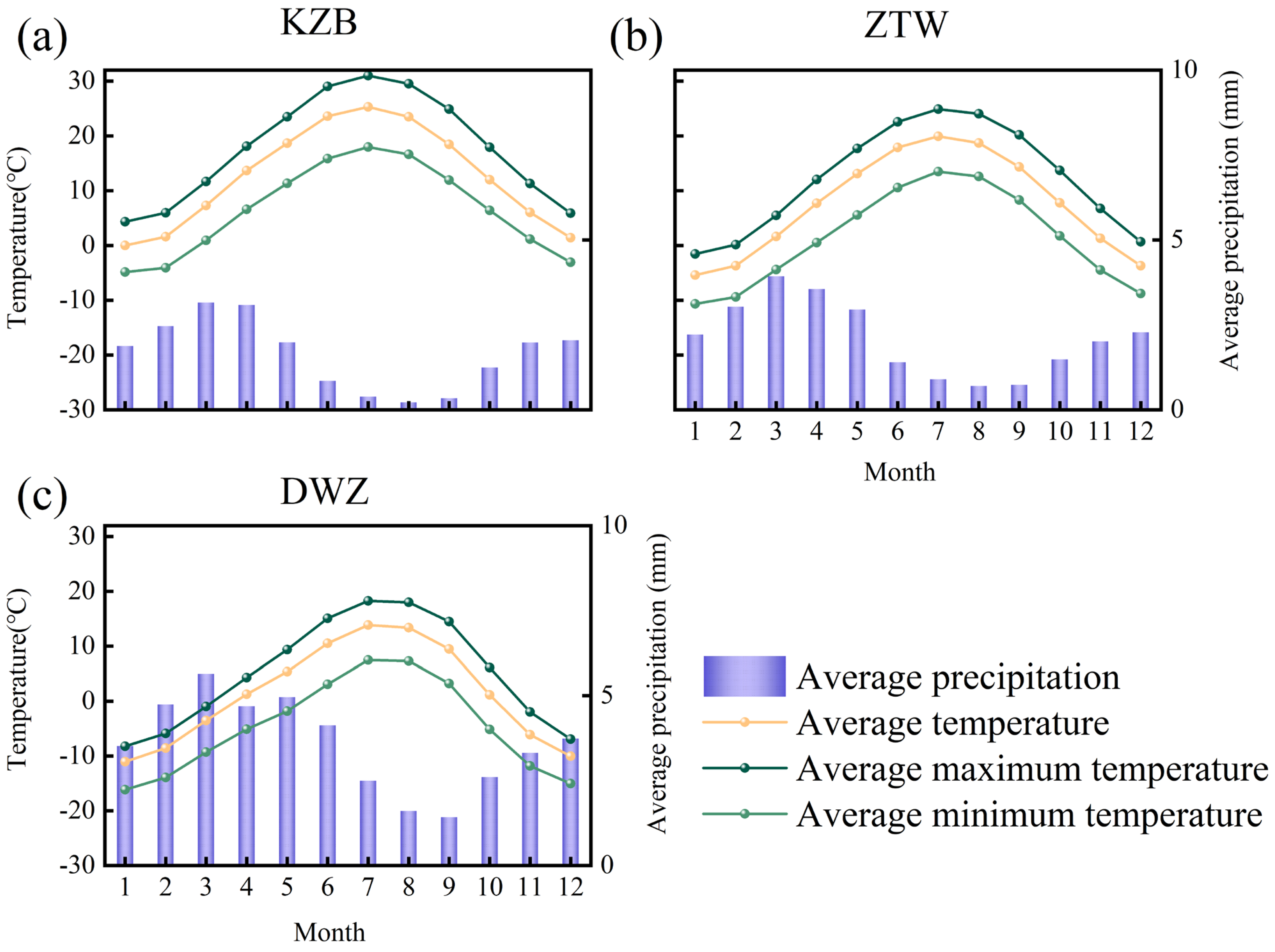
2.2.1. Climate Data
2.2.2. Tree-Ring Material
2.3. Remote Sensing Data
2.3.1. GIMMS NDVI
2.3.2. Remote Sensing Phenological Data
3. Method and Analysis
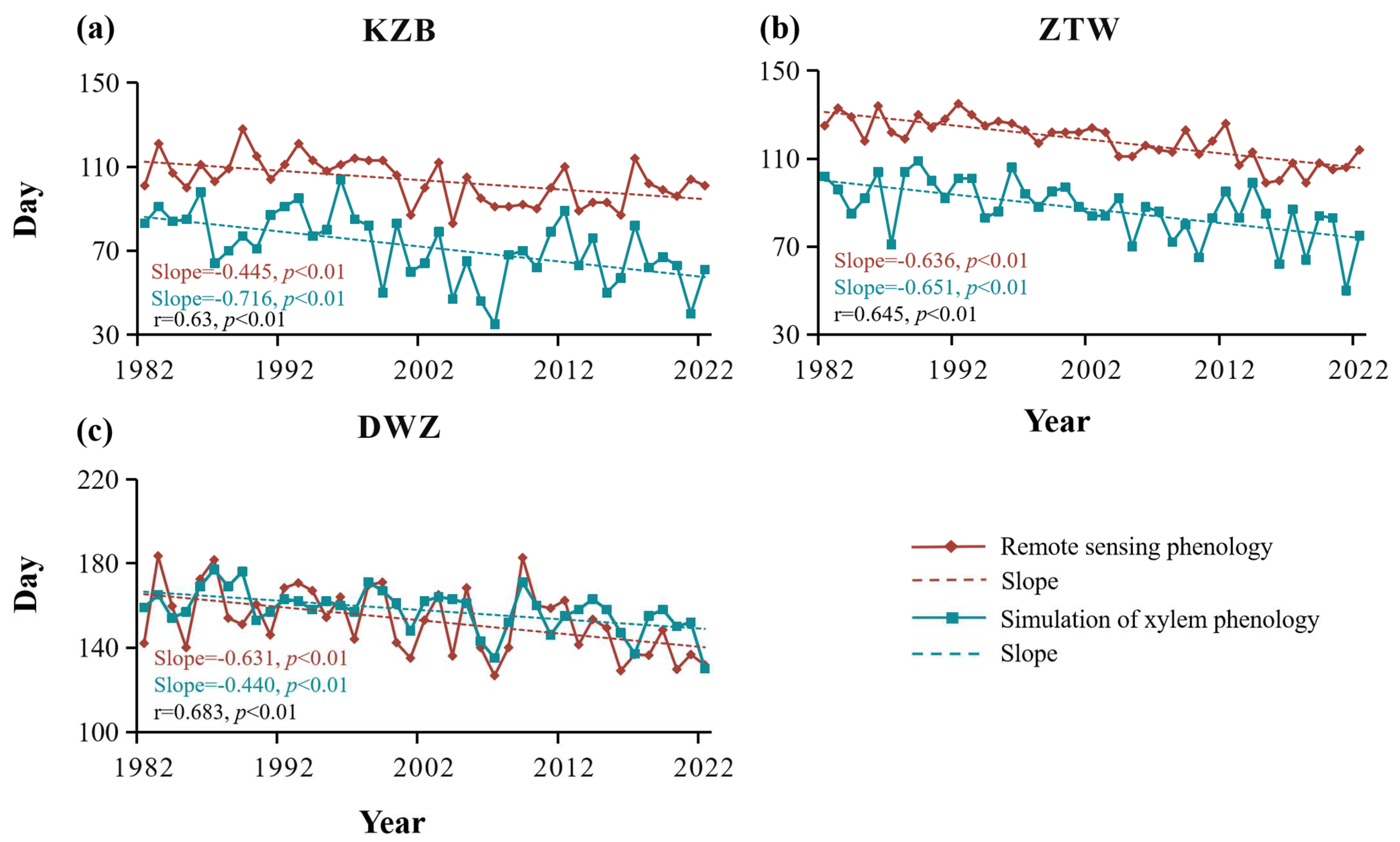
3.1. Simulation of Xylem Phenology and Determination of the Early Xylem Growth Season
3.1.1. Xylem Phenological Simulation
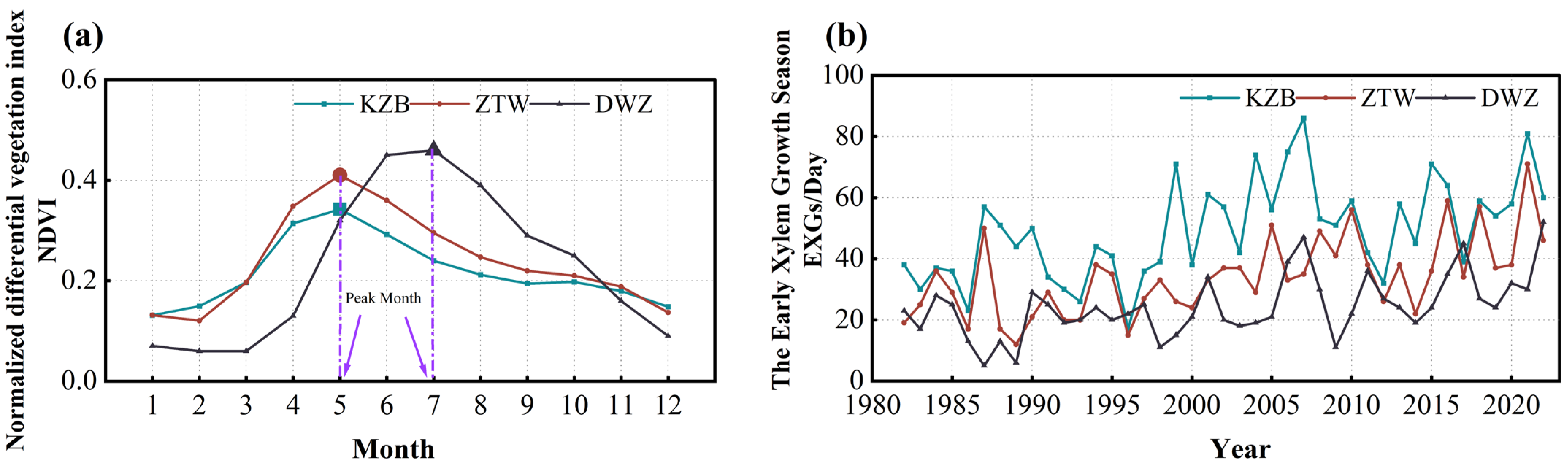
3.1.2. Determination of the Early Xylem Growth Season
3.2. Vector Autoregression Model
3.2.1. Impulse Response Analysis
3.2.2. Forecast Error Variance Decomposition
4. Results
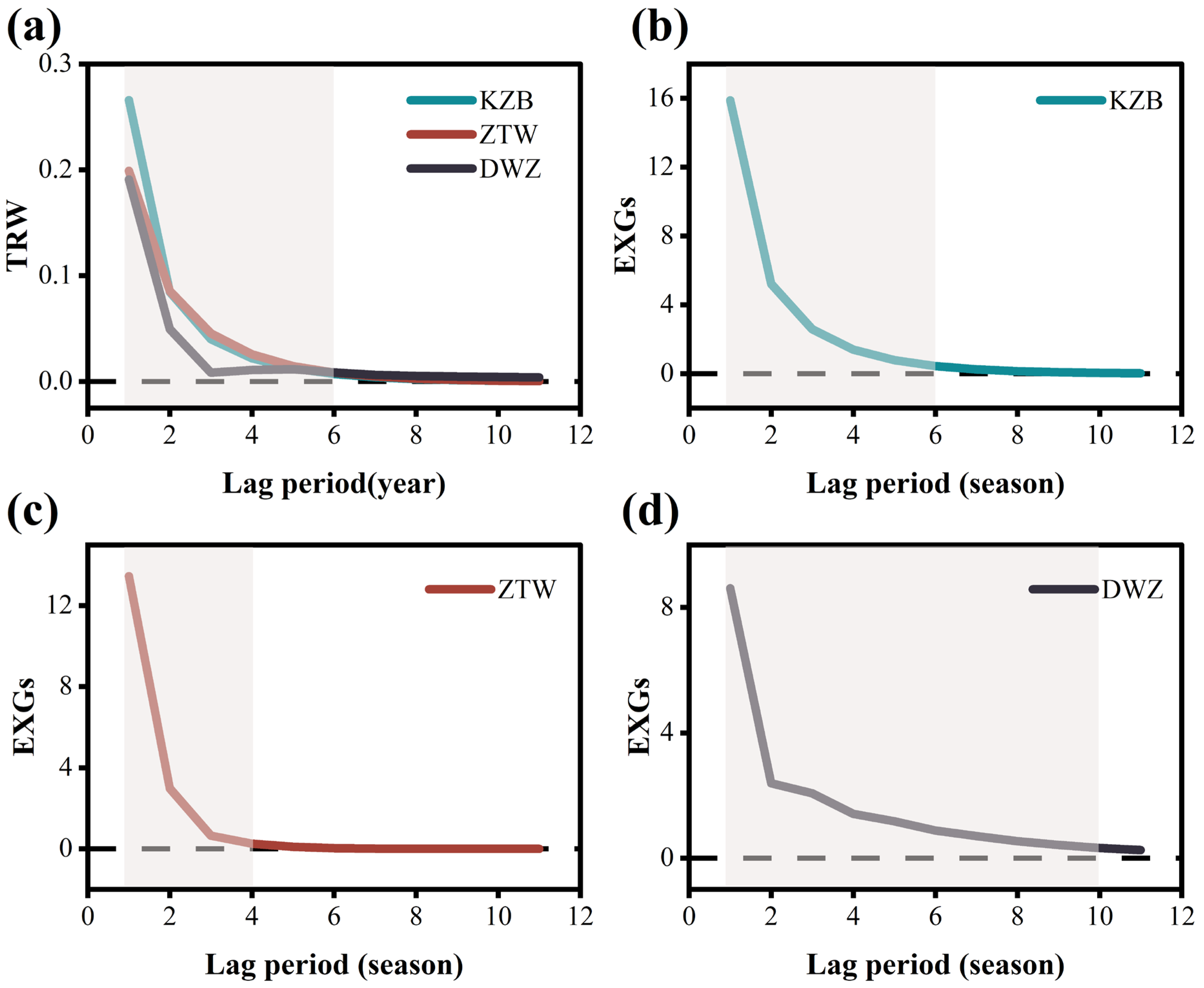
4.1. Xylem Vegetation Growth Carryover Effect
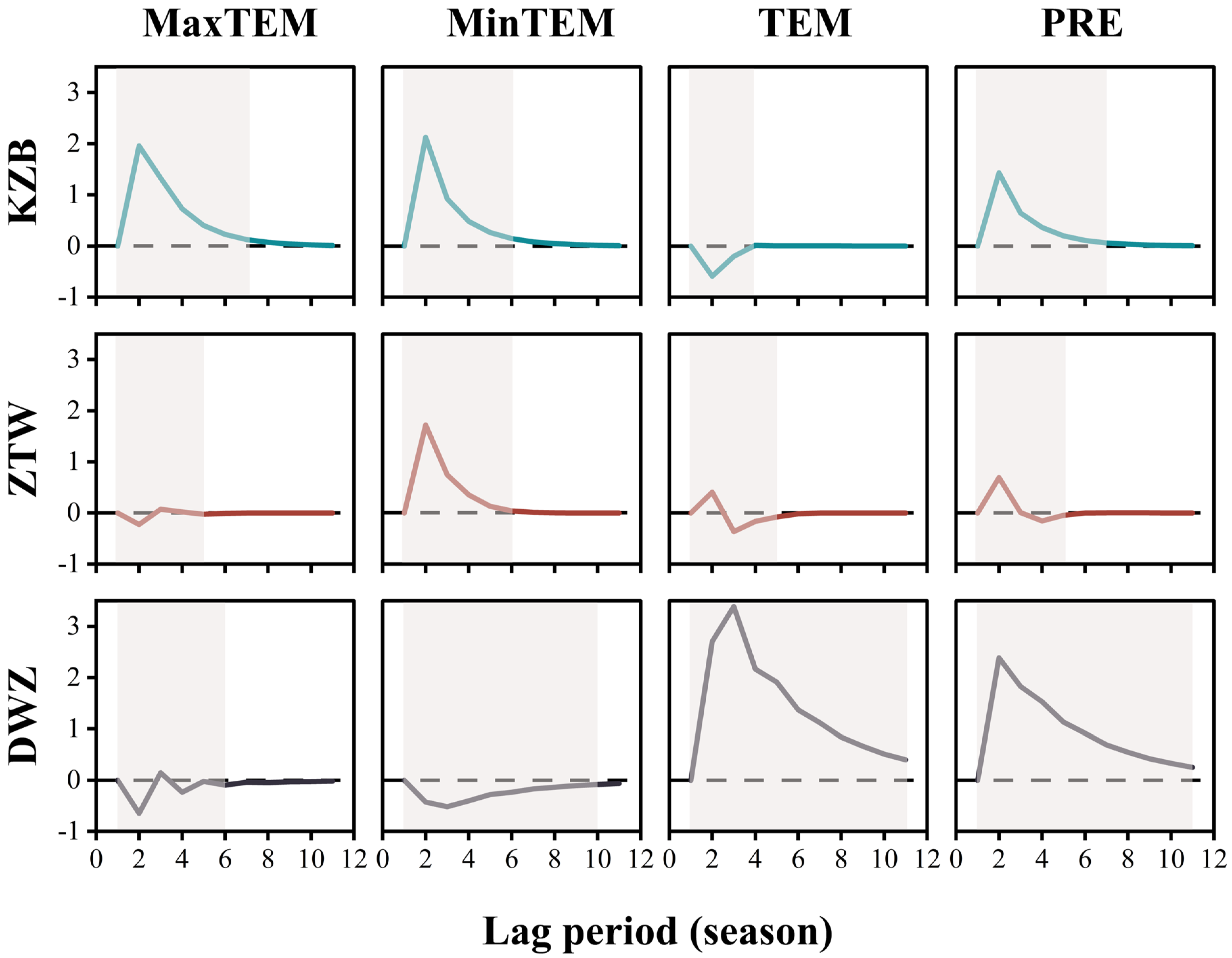
4.2. Lagged Climatic Effect Impact on Xylem
4.3. Effects of Lagged Climatic Effect and Vegetation Growth Carryover on Xylem
5. Discussion
5.1. Impact of Vegetation Growth Carryover and Lagged Climatic Effect on Growth Scale of Tree-Ring Width
5.2. Impact of Vegetation Growth Carryover and Lagged Climatic Effect on the Early Xylem Growth Season
5.3. The Impact of Xylem Vegetation Carryover and Lagged Climatic Effect on the Growth Strategy of Juniperus seravschanica
6. Conclusions and Research Uncertainties
6.1. Conclusions
6.2. Research Uncertainties
- (1)
- (2)
- The growth onset time simulated by the V-S model and the first day of the month with the maximum NDVI value are used to define the start of the peak growth period, thereby determining the time range of the early xylem growth season. However, this method involves cross-scale definitions and is subject to uncertainties.
Supplementary Materials
Author Contributions
Funding
Data Availability Statement
Acknowledgments
Conflicts of Interest
References
- Meyer, W.B.; Turner, B.L. Human population growth and global land-use/cover change. Annu. Rev. Ecol. Evol. Syst. 1992, 23, 39–61. [Google Scholar] [CrossRef]
- Nemani, R.R.; Keeling, C.D.; Hashimoto, H.; Jolly, W.M.; Piper, S.C.; Tucker, C.J.; Myneni, R.B.; Running, S.W. Climate-driven increases in global terrestrial net primary production from 1982 to 1999. Science 2003, 300, 1560–1563. [Google Scholar] [CrossRef]
- Silvestro, R.; Mencuccini, M.; García-Valdés, R.; Antonucci, S.; Arzac, A.; Biondi, F.; Buttò, V.; Camarero, J.J.; Campelo, F.; Cochard, H.J. Partial asynchrony of coniferous forest carbon sources and sinks at the intra-annual time scale. Nat. Commun. 2024, 15, 6169. [Google Scholar] [CrossRef]
- Heimann, M.; Reichstein, M.J.N. Terrestrial ecosystem carbon dynamics and climate feedbacks. Nature 2008, 451, 289–292. [Google Scholar] [CrossRef]
- Anderegg, W.R.; Schwalm, C.; Biondi, F.; Camarero, J.J.; Koch, G.; Litvak, M.; Ogle, K.; Shaw, J.D.; Shevliakova, E.; Williams, A.J.S. Pervasive drought legacies in forest ecosystems and their implications for carbon cycle models. Science 2015, 349, 528–532. [Google Scholar] [CrossRef]
- Anderegg, W.R.; Trugman, A.T.; Badgley, G.; Konings, A.G.; Shaw, J.J. Divergent forest sensitivity to repeated extreme droughts. Nat. Clim. Change 2020, 10, 1091–1095. [Google Scholar] [CrossRef]
- Liu, M.; Wang, H.; Zhai, H.; Zhang, X.; Shakir, M.; Ma, J.; Sun, W.; Meteorology, F. Identifying thresholds of time-lag and accumulative effects of extreme precipitation on major vegetation types at global scale. Agric. For. Meteorol. 2024, 358, 110239. [Google Scholar] [CrossRef]
- Wen, Y.; Liu, X.; Pei, F.; Li, X.; Du, G. Non-uniform time-lag effects of terrestrial vegetation responses to asymmetric warming. Agric. For. Meteorol. 2018, 252, 130–143. [Google Scholar] [CrossRef]
- Liu, Y.; Song, H.; Sun, C.; Song, Y.; Cai, Q.; Liu, R.; Lei, Y.; Li, Q. The 600-mm precipitation isoline distinguishes tree-ring-width responses to climate in China. Natl. Sci. Rev. 2019, 6, 359–368. [Google Scholar] [CrossRef]
- Wu, X.; Li, X.; Liu, H.; Ciais, P.; Li, Y.; Xu, C.; Babst, F.; Guo, W.; Hao, B.; Wang, P. Uneven winter snow influence on tree growth across temperate China. Glob. Change Biol. 2019, 25, 144–154. [Google Scholar] [CrossRef]
- Liu, H.; Park Williams, A.; Allen, C.D.; Guo, D.; Wu, X.; Anenkhonov, O.A.; Liang, E.; Sandanov, D.V.; Yin, Y.; Qi, Z. Rapid warming accelerates tree growth decline in semi-arid forests of Inner Asia. Glob. Change Biol. 2013, 19, 2500–2510. [Google Scholar] [CrossRef]
- Körner, C.J.S. A matter of tree longevity. Science 2017, 355, 130–131. [Google Scholar] [CrossRef]
- Babst, F.; Bodesheim, P.; Charney, N.; Friend, A.D.; Girardin, M.P.; Klesse, S.; Moore, D.J.; Seftigen, K.; Björklund, J.; Bouriaud, O. When tree rings go global: Challenges and opportunities for retro-and prospective insight. Quat. Sci. Rev. 2018, 197, 1–20. [Google Scholar] [CrossRef]
- Xue, H.; Shi, F.; Gennaretti, F.; Fu, Y.H.; He, B.; Wu, X.; Guo, Z. Evidence of advancing spring xylem phenology in Chinese forests under global warming. Sci. China Earth Sci. 2023, 66, 2187–2199. [Google Scholar] [CrossRef]
- Opała-Owczarek, M.; Owczarek, P.; Rahmonov, O.; Małarzewski, Ł.; Chen, F.; Niedźwiedź, T. Divergence in responses of juniper tree rings to climate conditions along a high-mountain transect in the semi-arid Fann Mountains, Pamirs-Alay, western Tajikistan. Ecol. Indic. 2023, 150, 110280. [Google Scholar] [CrossRef]
- Liu, Q.; Piao, S.; Janssens, I.A.; Fu, Y.; Peng, S.; Lian, X.; Ciais, P.; Myneni, R.B.; Peñuelas, J.; Wang, T.J.N.c. Extension of the growing season increases vegetation exposure to frost. Nat. Commun. 2018, 9, 426. [Google Scholar] [CrossRef]
- Lian, X.; Piao, S.; Chen, A.; Wang, K.; Li, X.; Buermann, W.; Huntingford, C.; Peñuelas, J.; Xu, H.; Myneni, R.B. Seasonal biological carryover dominates northern vegetation growth. Nat. Commun. 2021, 12, 983. [Google Scholar] [CrossRef]
- Lian, X.; Peñuelas, J.; Ryu, Y.; Piao, S.; Keenan, T.F.; Fang, J.; Yu, K.; Chen, A.; Zhang, Y.; Gentine, P. Diminishing carryover benefits of earlier spring vegetation growth. Nat. Ecol. Evol. 2024, 8, 218–228. [Google Scholar] [CrossRef]
- Wong, C.Y.; Young, D.J.; Latimer, A.M.; Buckley, T.N.; Magney, T.S. Importance of the legacy effect for assessing spatiotemporal correspondence between interannual tree-ring width and remote sensing products in the Sierra Nevada. Remote. Sens. Environ. 2021, 265, 112635. [Google Scholar] [CrossRef]
- Alfaro-Sánchez, R.; Nguyen, H.; Klesse, S.; Hudson, A.; Belmecheri, S.; Köse, N.; Diaz, H.; Monson, R.; Villalba, R.; Trouet, V. Climatic and volcanic forcing of tropical belt northern boundary over the past 800 years. Nat. Geosci. 2018, 11, 933–938. [Google Scholar] [CrossRef]
- Zhang, Z. Tree-rings, a key ecological indicator of environment and climate change. Ecol. Indic. 2015, 51, 107–116. [Google Scholar] [CrossRef]
- Tychkov, I.I.; Sviderskaya, I.V.; Babushkina, E.A.; Popkova, M.I.; Vaganov, E.A.; Shishov, V.V. How can the parameterization of a process-based model help us understand real tree-ring growth? Trees 2019, 33, 345–357. [Google Scholar] [CrossRef]
- Shishov, V.V.; Tychkov, I.I.; Popkova, M.I.; Ilyin, V.A.; Bryukhanova, M.V.; Kirdyanov, A.V. VS-oscilloscope: A new tool to parameterize tree radial growth based on climate conditions. Dendrochronologia 2016, 39, 42–50. [Google Scholar] [CrossRef]
- He, M.; Yang, B.; Wang, Z.; Bräuning, A.; Pourtahmasi, K.; Oladi, R. Climatic forcing of xylem formation in Qilian juniper on the northeastern Tibetan Plateau. Trees 2016, 30, 923–933. [Google Scholar] [CrossRef]
- Anchukaitis, K.J.; Evans, M.N.; Hughes, M.K.; Vaganov, E.A. An interpreted language implementation of the Vaganov–Shashkin tree-ring proxy system model. Dendrochronologia 2020, 60, 125677. [Google Scholar] [CrossRef]
- Kang, J.; Yang, Z.; Yu, B.; Ma, Q.; Jiang, S.; Shishov, V.V.; Zhou, P.; Huang, J.-G.; Ding, X.J.; Meteorology, F. An earlier start of growing season can affect tree radial growth through regulating cumulative growth rate. Agric. For. Meteorol. 2023, 342, 109738. [Google Scholar] [CrossRef]
- Jiao, L.; Jiang, Y.; Zhang, W.-T.; Wang, M.-C.; Zhang, L.-N.; Zhao, S.-D. Divergent responses to climate factors in the radial growth of Larix sibirica in the eastern Tianshan Mountains, northwest China. Trees 2015, 29, 1673–1686. [Google Scholar] [CrossRef]
- Fan, Y.; Shang, H.; Yu, S.; Wu, Y.; Li, Q. Understanding the representativeness of Tree rings and their Carbon isotopes in characterizing the Climate Signal of Tajikistan. Forests 2021, 12, 1215. [Google Scholar] [CrossRef]
- Gou, X.-X.; Zhang, T.-W.; Yu, S.-L.; Zhang, R.-B.; Jiang, S.-X.; Guo, Y.-L. Response of radial growth of Juniperus seravschanica to climate changes in different environmental conditions. J. Ecol. 2021, 40, 1574. [Google Scholar] [CrossRef]
- Kure, S.; Jang, S.; Ohara, N.; Kavvas, M.; Chen, Z. Hydrologic impact of regional climate change for the snow-fed and glacier-fed river basins in the Republic of Tajikistan: Statistical downscaling of global climate model projections. Hydrol. Process. 2013, 27, 4071–4090. [Google Scholar] [CrossRef]
- Nowak, A.; Nowak, S.; Nobis, M. The Pamirs-Alai mountains (middle Asia: Tajikistan). In Plant Biogeography and Vegetation of High Mountains of Central and South-West Asia; Springer: Berlin/Heidelberg, Germany, 2020; pp. 1–42. [Google Scholar] [CrossRef]
- Aalto, J.; Kämäräinen, M.; Shodmonov, M.; Rajabov, N.; Venäläinen, A. Features of Tajikistan's past and future climate. Int. J. Clim. 2017, 37, 4949–4961. [Google Scholar] [CrossRef]
- Kure, S.; Jang, S.; Ohara, N.; Kavvas, M.; Chen, Z. Hydrologic impact of regional climate change for the snowfed and glacierfed river basins in the Republic of Tajikistan: Hydrological response of flow to climate change. Hydrol. Process. 2013, 27, 4057–4070. [Google Scholar] [CrossRef]
- Yang, T.; Li, Q.; Chen, X.; De Maeyer, P.; Yan, X.; Liu, Y.; Zhao, T.; Li, L. Spatiotemporal variability of the precipitation concentration and diversity in Central Asia. Atmos. Res. 2020, 241, 104954. [Google Scholar] [CrossRef]
- Holmes, R.L. Computer-Assisted Quality Control in Tree-Ring Dating and Measurement; Tree-Ring Society: Tucson, AZ, USA, 1983. [Google Scholar]
- Huang, Y.; Jiang, N.; Shen, M.; Guo, L. Effect of preseason diurnal temperature range on the start of vegetation growing season in the Northern Hemisphere. Ecol. Indic. 2020, 112, 106161. [Google Scholar] [CrossRef]
- Chen, H.; Zhao, J.; Zhang, H.; Zhang, Z.; Guo, X.; Wang, M. Detection and attribution of the start of the growing season changes in the Northern Hemisphere. Sci. Total. Environ. 2023, 903, 166607. [Google Scholar] [CrossRef]
- Xu, X.; Riley, W.J.; Koven, C.D.; Jia, G.; Zhang, X. Earlier leaf-out warms air in the north. Nat. Clim. Change 2020, 10, 370–375. [Google Scholar] [CrossRef]
- Huang, J.; van den Dool, H.M.; Georgarakos, K.P. Analysis of model-calculated soil moisture over the United States (1931–1993) and applications to long-range temperature forecasts. J. Clim. 1996, 9, 1350–1362. [Google Scholar] [CrossRef]
- Furze, M.E.; Huggett, B.A.; Aubrecht, D.M.; Stolz, C.D.; Carbone, M.S.; Richardson, A.D. Whole-tree nonstructural carbohydrate storage and seasonal dynamics in five temperate species. New Phytol. 2019, 221, 1466–1477. [Google Scholar] [CrossRef]
- Hartmann, F.P.; Rathgeber, C.B.; Fournier, M.; Moulia, B.J. Modelling wood formation and structure: Power and limits of a morphogenetic gradient in controlling xylem cell proliferation and growth. Ann. For. Sci. 2017, 74, 14. [Google Scholar] [CrossRef]
- Antonucci, S.; Rossi, S.; Deslauriers, A.; Morin, H.; Lombardi, F.; Marchetti, M.; Tognetti, R.J.A.; Meteorology, F. Large-scale estimation of xylem phenology in black spruce through remote sensing. Agric. For. Meteorol. 2017, 233, 92–100. [Google Scholar] [CrossRef]
- Huang, J.G.; Deslauriers, A.; Rossi, S.J.N.P. Xylem formation can be modeled statistically as a function of primary growth and cambium activity. New Phytol. 2014, 203, 831–841. [Google Scholar] [CrossRef]
- Yang, B.; He, M.; Shishov, V.; Tychkov, I.; Vaganov, E.; Rossi, S.; Ljungqvist, F.C.; Bräuning, A.; Grießinger, J.J.P.o.t.N.A.o.S. New perspective on spring vegetation phenology and global climate change based on Tibetan Plateau tree-ring data. Proc. Natl. Acad. Sci. USA 2017, 114, 6966–6971. [Google Scholar] [CrossRef]
- Piermattei, A.J. A new perspective on tree growing season determination. J. Biogeogr. 2024, 51, 2334–2337. [Google Scholar] [CrossRef]
- Tang, W.; Liu, S.; Jing, M.; Healey, J.R.; Smith, M.N.; Farooq, T.H.; Zhu, L.; Zhao, S.; Wu, Y. Vegetation growth responses to climate change: A cross-scale analysis of biological memory and time lags using tree ring and satellite data. Glob. Change Biol. 2024, 30, e17441. [Google Scholar] [CrossRef]
- Tang, W.; Liu, S.; Kang, P.; Peng, X.; Li, Y.; Guo, R.; Jia, J.; Liu, M.; Zhu, L. Quantifying the lagged effects of climate factors on vegetation growth in 32 major cities of China. Ecol. Indic. 2021, 132, 108290. [Google Scholar] [CrossRef]
- Lee, C.-C.; Chang, C.-P. New evidence on the convergence of per capita carbon dioxide emissions from panel seemingly unrelated regressions augmented Dickey–Fuller tests. Energy 2008, 33, 1468–1475. [Google Scholar] [CrossRef]
- Maziarz, M. A review of the Granger-causality fallacy. J. Philos. Econ. Reflect. Econ. Soc. Issues 2015, 8, 86–105. [Google Scholar] [CrossRef]
- Hansen, P.R. Structural changes in the cointegrated vector autoregressive model. J. Econ. 2003, 114, 261–295. [Google Scholar] [CrossRef]
- Lütkepohl, H. Vector autoregressive models. In Handbook of Research Methods and Applications in Empirical Macroeconomics; Edward Elgar Publishing: Cheltenham, UK, 2013; pp. 139–164. [Google Scholar]
- Haslbeck, J.M.; Bringmann, L.F.; Waldorp, L.J. A tutorial on estimating time-varying vector autoregressive models. Multivar. Behav. Res. 2021, 56, 120–149. [Google Scholar] [CrossRef]
- Volpicella, A.J.; Statistics, E. SVARs identification through bounds on the forecast error variance. J. Bus. Econ. Stat. 2022, 40, 1291–1301. [Google Scholar] [CrossRef]
- Gujarati, D.N. Essentials of Econometrics; Sage Publications: Thousand Oaks, CA, USA, 2021. [Google Scholar]
- Yuan, Y.; Bao, A.; Jiapaer, G.; Jiang, L.; De Maeyer, P.J. Phenology-based seasonal terrestrial vegetation growth response to climate variability with consideration of cumulative effect and biological carryover. Sci. Total. Environ. 2022, 817, 152805. [Google Scholar] [CrossRef]
- Zhang, X.; Cao, Q.; Chen, H.; Quan, Q.; Li, C.; Dong, J.; Chang, M.; Yan, S.; Liu, J. Effect of vegetation carryover and climate variability on the seasonal growth of vegetation in the upper and middle reaches of the Yellow River Basin. Remote. Sens. 2022, 14, 5011. [Google Scholar] [CrossRef]
- Huang, M.; Wang, X.; Keenan, T.F.; Piao, S.J. Drought timing influences the legacy of tree growth recovery. Glob. Change Biol. 2018, 24, 3546–3559. [Google Scholar] [CrossRef]
- Gao, S.; Liang, E.; Liu, R.; Babst, F.; Camarero, J.J.; Fu, Y.H.; Piao, S.; Rossi, S.; Shen, M.; Wang, T.J.; et al. An earlier start of the thermal growing season enhances tree growth in cold humid areas but not in dry areas. Nat. Ecol. Evol. 2022, 6, 397–404. [Google Scholar] [CrossRef]
- Wu, G.; Xu, G.; Chen, T.; Liu, X.; Zhang, Y.; An, W.; Wang, W.; Fang, Z.-A.; Yu, S.J. Age-dependent tree-ring growth responses of Schrenk spruce (Picea schrenkiana) to climate—A case study in the Tianshan Mountain, China. Dendrochronologia 2013, 31, 318–326. [Google Scholar] [CrossRef]
- Lavergne, A.; Daux, V.; Villalba, R.; Barichivich, J. Temporal changes in climatic limitation of tree-growth at upper treeline forests: Contrasted responses along the west-to-east humidity gradient in Northern Patagonia. Dendrochronologia 2015, 36, 49–59. [Google Scholar] [CrossRef]
- Gou, X.; Zhang, T.; Yu, S.; Liu, K.; Zhang, R.; Shang, H.; Qin, L.; Fan, Y.; Jiang, S.; Zhang, H. Climate response of Picea schrenkiana based on tree-ring width and maximum density. Dendrochronologia 2023, 78, 126067. [Google Scholar] [CrossRef]
- Zhang, H.; Cai, Q.; Liu, Y. Altitudinal difference of growth-climate response models in the north subtropical forests of China. Dendrochronologia 2022, 72, 125935. [Google Scholar] [CrossRef]
- Liu, Q.; Fu, Y.H.; Zhu, Z.; Liu, Y.; Liu, Z.; Huang, M.; Janssens, I.A.; Piao, S.J. Delayed autumn phenology in the Northern Hemisphere is related to change in both climate and spring phenology. Glob. Change Biol. 2016, 22, 3702–3711. [Google Scholar] [CrossRef]
- Schwartz, M.D.; Ahas, R.; Aasa, A.J. Onset of spring starting earlier across the Northern Hemisphere. Glob. Change Biol. 2006, 12, 343–351. [Google Scholar] [CrossRef]
- Keeling, C.D.; Chin, J.; Whorf, T.J.N. Increased activity of northern vegetation inferred from atmospheric CO2 measurements. Nature 1996, 382, 146–149. [Google Scholar] [CrossRef]
- Piao, S.; Friedlingstein, P.; Ciais, P.; Viovy, N.; Demarty, J. Growing season extension and its impact on terrestrial carbon cycle in the Northern Hemisphere over the past 2 decades. Glob. Biogeochem. Cycles 2007, 21, 22151–22156. [Google Scholar] [CrossRef]
- Yu, H.; Luedeling, E.; Xu, J. Winter and spring warming result in delayed spring phenology on the Tibetan Plateau. Proc. Natl. Acad. Sci. USA 2010, 107, 22151–22156. [Google Scholar] [CrossRef]
- Liu, N.; Peng, S.-Z.; Chen, Y.-M. Temporal effects of climate factors on vegetation growth on the Qingzang Plateau, China. Chin. J. Plan Ecol. 2022, 46, 18. [Google Scholar] [CrossRef]
- Li, Y.; Chen, Y. The continuing shrinkage of snow cover in High Mountain Asia over the last four decades. In Proceedings of the EGU General Assembly Conference Abstracts, Vienna, Austria, 23–28 August 2023; p. EGU–16661. [Google Scholar]
- Wang, X.; Wang, T.; Guo, H.; Liu, D.; Zhao, Y.; Zhang, T.; Liu, Q.; Piao, S. Disentangling the mechanisms behind winter snow impact on vegetation activity in northern ecosystems. Glob. Change Biol. 2018, 24, 1651–1662. [Google Scholar] [CrossRef]
- Jiang, B.; Shi, Y.; Peng, Y.; Jia, Y.; Yan, Y.; Dong, X.; Li, H.; Dong, J.; Li, J.; Gong, Z.J. Cold-induced CBF–PIF3 interaction enhances freezing tolerance by stabilizing the phyB thermosensor in Arabidopsis. Mol. Plant 2020, 13, 894–906. [Google Scholar] [CrossRef]
- Che, C.; Xiao, S.; Peng, X.; Ding, A.; Su, J. Radial growth of Korshinsk peashrub and its response to drought in different sub-arid climate regions of northwest China. J. Environ. Manag. 2023, 326, 116708. [Google Scholar] [CrossRef]
- Esper, J. Long-term tree-ring variations in Juniperus at the upper timber-line in the Karakorum (Pakistan). Holocene 2000, 10, 253–260. [Google Scholar] [CrossRef]
- Esper, J.; Cook, E.R.; Krusic, P.J.; Peters, K.; Schweingruber, F.H. Tests of the RCS method for preserving low-frequency variability in long tree-ring chronologies. Tree-Ring Res. 2003, 59, 81–98. [Google Scholar]
- Esper, J.; Frank, D.C.; Wilson, R.J.; Büntgen, U.; Treydte, K.J.T. Uniform growth trends among central Asian low-and high-elevation juniper tree sites. Trees 2007, 21, 141–150. [Google Scholar] [CrossRef]
- Vaganov, E.A.; Hughes, M.K.; Shashkin, A.V. Growth Dynamics of Conifer Tree Rings: Images of Past and Future Environments; Springer Science & Business Media: Berlin/Heidelberg, Germany, 2006; Volume 183. [Google Scholar]
- Tumajer, J.; Kašpar, J.; Kuželová, H.; Shishov, V.V.; Tychkov, I.I.; Popkova, M.I.; Vaganov, E.A.; Treml, V.J. Forward modeling reveals multidecadal trends in cambial kinetics and phenology at treeline. Front. Plant Sci. 2021, 12, 613643. [Google Scholar] [CrossRef]


| Type | KZB | ZTW | DWZ |
|---|---|---|---|
| Latitude | 40.646455° N | 39.3531° N | 38.586636° N |
| Longitude | 69.612838° E | 67.510412° E | 70.857156° E |
| Altitude/m | 1575.7 | 2147.1 | 2073 |
| Slope direction | S | N | WS |
| Sample core/tree | 52/26 | 40/20 | 39/21 |
| Sample depth | 1896–2023 | 1846–2023 | 1929–2023 |
| The first year of subsample signal strength (SSS > 0.85) | 1896 | 1846 | 1929 |
| Standard deviation (SD) | 0.247 | 0.361 | 0.193 |
| Mean sensitivity (MS) | 0.200 | 0.279 | 0.196 |
| Mean correlation coefficient among all series (R1) | 0.284 | 0.225 | 0.195 |
| Mean correlation coefficient between trees (R2) | 0.270 | 0.203 | 0.160 |
| Mean correlation coefficient within trees (R3) | 0.821 | 0.787 | 0.659 |
| Express population signal (EPS) | 0.936 | 0.883 | 0.882 |
| Signal-to-noise ratio (SNR) | 14.50 | 17.55 | 17.51 |
Disclaimer/Publisher’s Note: The statements, opinions and data contained in all publications are solely those of the individual author(s) and contributor(s) and not of MDPI and/or the editor(s). MDPI and/or the editor(s) disclaim responsibility for any injury to people or property resulting from any ideas, methods, instructions or products referred to in the content. |
© 2025 by the authors. Licensee MDPI, Basel, Switzerland. This article is an open access article distributed under the terms and conditions of the Creative Commons Attribution (CC BY) license (https://creativecommons.org/licenses/by/4.0/).
Share and Cite
Chen, J.; Wang, Y.; Zhang, T.; Liu, K.; Guo, K.; Hou, T.; Song, J.; He, Z.; Liang, B. Vegetation Growth Carryover and Lagged Climatic Effect at Different Scales: From Tree Rings to the Early Xylem Growth Season. Forests 2025, 16, 1107. https://doi.org/10.3390/f16071107
Chen J, Wang Y, Zhang T, Liu K, Guo K, Hou T, Song J, He Z, Liang B. Vegetation Growth Carryover and Lagged Climatic Effect at Different Scales: From Tree Rings to the Early Xylem Growth Season. Forests. 2025; 16(7):1107. https://doi.org/10.3390/f16071107
Chicago/Turabian StyleChen, Jiuqi, Yonghui Wang, Tongwen Zhang, Kexiang Liu, Kailong Guo, Tianhao Hou, Jinghui Song, Zhihao He, and Beihua Liang. 2025. "Vegetation Growth Carryover and Lagged Climatic Effect at Different Scales: From Tree Rings to the Early Xylem Growth Season" Forests 16, no. 7: 1107. https://doi.org/10.3390/f16071107
APA StyleChen, J., Wang, Y., Zhang, T., Liu, K., Guo, K., Hou, T., Song, J., He, Z., & Liang, B. (2025). Vegetation Growth Carryover and Lagged Climatic Effect at Different Scales: From Tree Rings to the Early Xylem Growth Season. Forests, 16(7), 1107. https://doi.org/10.3390/f16071107