Quantifying the Independent and Interactive Effects of Environmental Drivers on Dry-Day Evapotranspiration Between Two Slope Positions in a Larch Forest

Abstract

Differences in environmental conditions due to slope topography result in differences in evapotranspiration along slopes, but it is unclear how changes in environmental conditions affect the variations in evapotranspiration along slopes. Therefore, we monitored dry-day evapotranspiration (ET_d), solar radiation, vapor pressure deficit (VPD), and soil moisture downslope and upslope on a larch plantation hillslope from July to September 2023 to reveal the mechanisms driving ET_d variations. The results revealed that the difference in ET_d values between the downslope and upslope positions varied by month, with comparable ET_d values at both positions in July and higher ET_d values at the downslope position than at the upslope position in August and September. An ET_d model combining the effects of solar radiation, VPD, and soil water content was developed, which explained 68% of the variation in ET_d. The contributions of solar radiation, VPD, soil moisture, and their interactions to ET_d varied across slope positions, and ET_d was limited mainly by solar radiation downslope and by soil moisture upslope. Our study improves the understanding of the mechanisms governing the variations in evapotranspiration along slopes, and provides a new methodology for quantifying the effects of environmental differences between slope positions on evapotranspiration.

1. Introduction

Evapotranspiration (ET) is an important component of the water balance of forest ecosystems, and changes in ET have important implications for runoff and water allocation [1,2]. In water-limited areas, the conflict between large-scale afforestation and limited water resources is particularly acute and requires scientific management of water in forests [3]. The management of water in forests involves optimizing ET processes through vegetation structure regulation, thereby achieving runoff regulation and watershed water allocation [4]. Hillslopes, which are fundamental watershed units, are critical for forest-water management. Effective management necessitates the consideration of hillslope-specific vegetation carrying capacities, which are influenced by vegetation water use, as well as a more accurate estimation of slope ET. Topography-induced variations in environmental conditions (e.g., vapor pressure deficit and soil moisture) lead to obvious differences in water use across slope positions [5]. These differences not only influence water movement and distribution along hillslopes but also further alter watershed hydrological processes. For example, several studies reported that variations in ET due to slope position differences can reach 40%, posing substantial challenges for slope ET estimation and watershed water resource management [6,7]. In addition, although most watershed hydrological models incorporate basic topographic factors to estimate evapotranspiration, they still inadequately represent spatial heterogeneity at the hillslope scale due to some unresolved issues. These issues include treating hillslopes as homogeneous units while ignoring variations in topography, microclimate, and vegetation across different slope positions, and oversimplifying the transition in scale from plot to hillslope by extrapolating measurements from a single slope position to represent an entire hillslope [8,9]. This limitation is particularly critical in forested hillslopes with complex terrain, where ET variability primarily stems from microtopography-mediated variations in microclimate and soil moisture. However, current research on forest ET predominantly focuses on plot/stand or watershed scales [10,11], understanding of hillslope-scale ET mechanisms remains limited, especially concerning how ET spatiotemporal patterns respond to topography-driven microclimate and soil moisture variations.

Forest evapotranspiration can be broadly divided into evapotranspiration (transpiration and forest floor evapotranspiration) on dry days and evaporation due to interception on rainy days [2,12]. At a global scale, evaporation due to interception is relatively low (approximately 10% of the total ET) [13]; therefore, dry-day ET is the main mode of water use in forests. Numerous studies have investigated on the mechanisms affecting the temporal dynamics of evapotranspiration. Meteorological conditions, particularly solar radiation and vapor pressure deficit (VPD), are the main drivers of the variation in evapotranspiration [14,15], but their relationships vary with environmental conditions (e.g., water conditions). For example, VPD clearly has a negative effect on evapotranspiration in water-limited forests, whereas evapotranspiration usually increases with VPD in subtropical and tropical forests with favorable moisture conditions [14,16]. Soil moisture also plays a key role in regulating evapotranspiration [17]. Jung et al. [18] reported that a decrease in soil water content led to a decline in evapotranspiration at the global scale; however, the relationship between soil moisture and evapotranspiration is diverse at small to medium scales (e.g., regional, watershed, and slope scales), and is influenced primarily by vegetation cover types and the spatial heterogeneity of soil moisture [19]. Overall, existing research has focused primarily on the mechanisms driving the temporal dynamics of evapotranspiration, with most findings derived from plot/stand and region-scale observations. However, whether these conclusions are applicable at the hillslope scale remains insufficiently validated and explored. Additionally, although some studies have preliminarily identified the dominant factors influencing evapotranspiration variations across slope positions, these investigations have largely remained at the qualitative level and lack in-depth quantitative analysis [20,21,22]. Although many previous studies have used path analysis, correlation analysis, and linear perturbation analysis to quantify the contributions of factors to evapotranspiration [23,24,25], how dominant factors interact across different slope positions, and the extent to which variations in these factors contribute to differences in evapotranspiration, remain unclear.

In practice, hillslope evapotranspiration (and its components) observations are typically divided into 2–3 slope positions [26,27] owing to the complexity of spatial heterogeneity on hillslopes and practical constraints such as the number of instruments and installation challenges. However, the limited number of observational samples increases the difficulty of quantifying the differential impacts of key factors across slope positions on evapotranspiration. Therefore, there is an urgent need to develop a simple yet practical approach to address this current research challenge. Models are typically multifunctional, capable of not only simulating and predicting but also addressing issues that cannot be directly resolved through limited observational data. Therefore, quantifying the differential impacts of key factors across slope positions on evapotranspiration using evapotranspiration models may serve as an effective approach, particularly through empirical models that integrate the effects of dominant factors. Several stand-scale multifactorial models, such as the evapotranspiration model established on the basis of the Jarvis–Stewart equation, which considers the effects of meteorological factors and soil moisture, have been developed at the stand scale [28]. Since the influence of dominant factors may have scaled effects [29], the model structure developed at the stand scale may not necessarily be adapted to the hillslope scale, coupled with the fact that there is very little development in slope-scale evapotranspiration models. Therefore, to accurately quantify and understand the differential impacts of key factors across slope positions on evapotranspiration, it is essential to further develop corresponding tools or quantitative methods based on the development or improvement of hillslope-scale evapotranspiration models coupled with the effects of key factors.

Larix gmelinii var. principis-rupprechtii (Mayr) Pilg. (larch) is a major silvicultural species in northern China, especially in the Liupan Mountains region. However, most afforested areas in this region are on hillslopes, and the slope variations in environmental conditions would lead to differences in water use. Therefore, an in-depth understanding of the spatial variation in evapotranspiration along slopes and its mechanisms of variation is valuable for forest and water management in this region. In this study, we selected larch plantations at two slope positions (downslope and upslope) to observe dry-day evapotranspiration (ET_d), meteorology, and soil water content simultaneously, with the main objectives of (1) clarifying the differences in ET_d and their variations between the two slope positions, (2) developing a methodological framework to differentiate the contributions of individual dominant factor to ET_d at the hillslope scale, and (3) quantifying the contributions of each dominant factor and their interactions to ET_d at different slope positions.

2. Materials and Methods

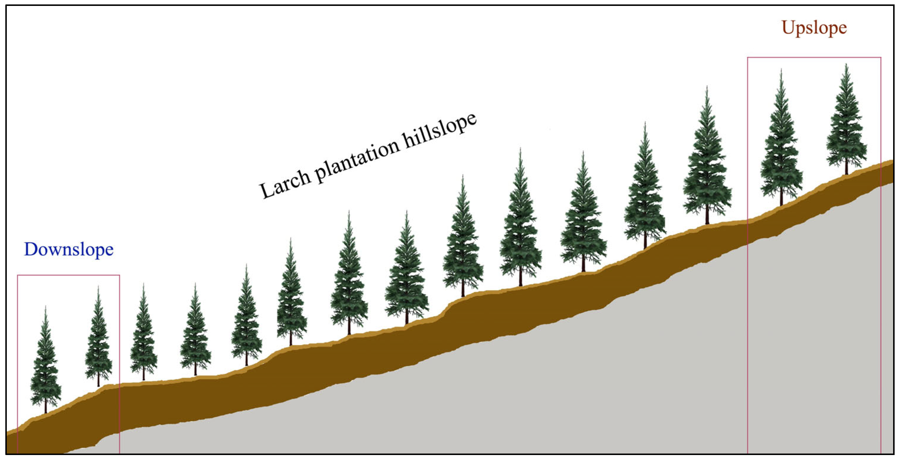
2.1. Study Site and Hillslope Description

The study area is located in the Xiangshuihe small watershed (106°12′–106°16′ E, 35°27′–35°33′ N, 2010–2942 m), covering an area of 43.7 km² south of the Liupan Mountains Nature Reserve (LMNS) of the Ningxia Hui Autonomous Region. The climate is warm–temperate and semihumid, with an average annual temperature of 5.8 °C and an average annual precipitation of 618 mm (1981–2010). The soils are dominated by haplic grayxems. The vegetation types are mainly natural secondary forests and plantations, and the species of natural secondary forests include Pinus armandii Franch., Betula albosinensis Burkill, Betula platyphylla Sukaczev, and Quercus liaotungensis Koidz.. The species of plantation is dominated by Larix gmelinii var. principis-rupprechtii, with a small amount of Pinus tabuliformis Carrière.

In the small watershed, a typical southeast-facing, same-age pure larch plantation (planted in 1981) on a hillslope ranging from 2265 m to 2483 m above sea level (a.s.l.) was established, with an average slope gradient of 27.8°. The understorey shrub cover was approximately 5%, dominated by Viburnum mongolicum (Pall.) Rehder and Berberis circumserrata (Schneid.) Schneid. The herbaceous cover was approximately 40%, dominated by Fragaria orientalis Losinsk. and Carex hancokiana Maxim.. To carry out this experiment, a 30 m × 30 m sample plot was established at both the bottom and top of the slope, with the two plots separated horizontally by approximately 400 m (Figure 1). Owing to strict protection and management, the studied hillslope, which is located within the LMNS, has not experienced significant human interference (e.g., thinning and fertilization) or natural disasters (e.g., pest infestations and fires). The experiment was carried out from 1 July to 30 September 2023. The basic stand information and the soil characteristics of each sample plot downslope and upslope are given in

Table 1. Stand information and soil properties of the 0–60 cm soil layer of the two downslope and upslope plots.

Characteristic	Downslope	Upslope
Elevation (m)	2279	2472
Slope gradient (°)	34	26
Stand density (stem·ha−1)	933	944
Mean DBH (cm)	18.9 ± 3.7	20.6 ± 4.0
Mean tree height (m)	16.3 ± 3.5	16.9 ± 2.9
Mean leaf area index (m2·m−2)	2.96 ± 0.40	3.59 ± 0.36
Soil depth (m)	1.2	1.0
Soil bulk density (g·cm−3)	1.10	0.94
Soil water holding capacity (%)	33.5	37.7
Soil wilting point (%)	17.6	15.5
Clay (%)	13.1	11.6
Silt (%)	62.1	66.4
Sand (%)	24.8	22.0

Note: Soil physical properties were determined using the cutting ring core sampling method. The soil wilting point data were obtained from adjacent sample plots at each slope position.

.

2.2. Meteorological and Soil Moisture Measurements

ATMOS-41 integrated weather stations (Meter, Pullman, WA, USA) were installed above the stands in the two sample plots downslope and upslope to measure the air temperature (T_a, °C), relative humidity (RH, %), solar radiation intensity (R_s, w·m⁻²), and wind speed (u, m·s⁻¹), with sensors located approximately 22 m above the forest floor. Data were recorded every 10 min using a CR1000X data collector (Campbell, Logan, UT, USA). The VPD (kPa) was calculated from the observed air temperature and relative humidity using the following formula:

$$VPD=0.611\times (1-{\displaystyle \frac{RH}{100}})\times \mathrm{e}\mathrm{x}\mathrm{p}\left({\displaystyle \frac{17.502T_{\mathrm{a}}}{T_{\mathrm{a}}+240.97}}\right)$$

(1)

Soil moisture and temperature sensors (ML3, Delta-T Devices, Cambridge, UK) were deployed in the 0–10, 10–20, 20–40, and 40–60 soil layers in two sample plots downslope and upslope to monitor the volumetric soil water content (SWC), and the data were recorded at 10 min intervals using a CR1000X data collector. The SWC in the 0–60 cm soil layer was the weighted average of the SWC in each layer.

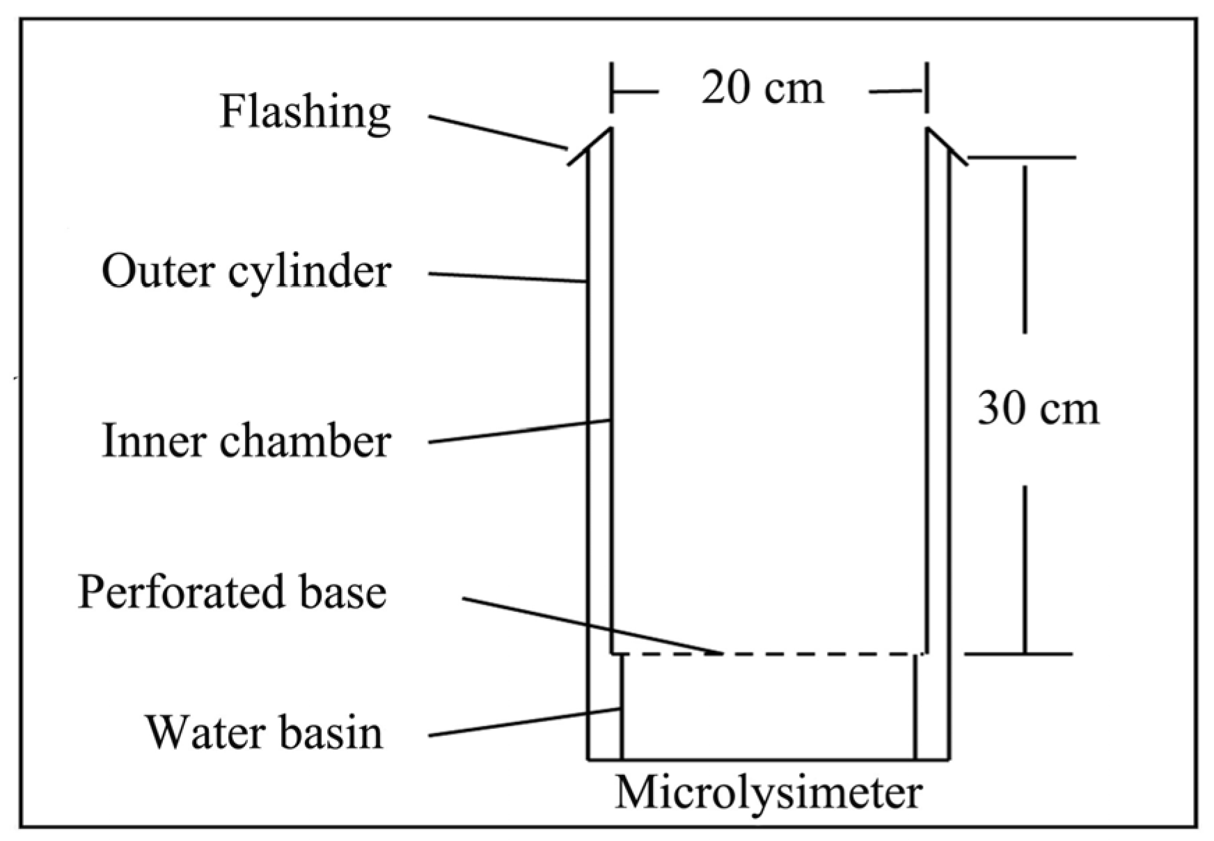
2.3. Evapotranspiration Component Measurements and Evapotranspiration Estimation

A previous study in the larch plantation at our study site suggested that a minimum of six sample trees should be secured for sap flow measurements to ensure reliable stand-scale sap flux estimates when stand densities are greater than 933 stem·ha⁻¹ [30]. Thus, three sample trees were randomly selected per DBH diameter class (DBH ≤ 19.0 cm and DBH > 19.0 cm) for sap flow measurements in each sample plot (

Table 2. Characteristics of the sample trees at the two slope positions.

Slope Position	Tree Code	DBH (cm)	Tree Height (m)	Sapwood Area (cm2)
Downslope	1	12.9	13.9	72.5
	2	14.5	14.5	87.2
	3	14.9	14.7	91.1
	4	19.2	16.4	136.0
	5	24.1	18.3	194.7
	6	28.2	19.9	249.6
Upslope	1	13.9	14.2	72.6
	2	16.3	15.3	98.5
	3	19.0	16.4	132.2
	4	21.0	17.1	160.2
	5	24.2	18.0	210.4
	6	27.4	18.8	267.0

). The sap flow of the sample trees was observed using the thermal dissipation probes with four 20 mm-long sensors, and the data were recorded every 10 min using a CR1000X data collector. The sensors were positioned on the north side of the tree trunks (the side not exposed to direct sunlight) at a height of 1.3 m above the ground, with the sensors inserted into the sapwood to a depth of 20 mm. The measured temperature differences were converted to sap flux density via Baseline software (version 3.0.7, Yavor Parashkevov, Duke University, Durham, NC, USA) using the calibration Granier formula (Equation (2)), which has been widely used in larch plantations [31]. Furthermore, a synthesis of 290 calibration experiments revealed that species differences accounted for only a small proportion of the calibration variability [32], confirming the validity of the calibration parameters of the Granier formula for sap flow measurements in larch plantations.

$$J_{\mathrm{s}0-20}=0.714\times {({\displaystyle \frac{∆T_{\mathrm{m}}}{∆T}}-1)}^{1.231}$$

(2)

where J_s0–20 (mL·cm⁻²·min⁻¹) is the sap flux density at a 0–20 sapwood depth; ΔT_m (°C) is the maximum temperature difference when the sap flow is close to zero, which can be determined by Baseline software; and ΔT (°C) is the actual temperature difference corrected using Equation (3):

$$∆T=∆T_0-{\displaystyle \frac{\left(∆T_1+∆T_2\right)}{2}}$$

(3)

where ΔT₀, ΔT₁, and ΔT₂ (°C) are the temperature differences between sensors S₀ and S₁, between sensors S₂ and S₁, and between sensors S₃ and S₁, respectively.

When the sapwood depth of the sample trees exceeded 20 mm, the sap flux density at the 20–40 mm sapwood depth (J_s20–40, mL·cm⁻²·min⁻¹) was calculated on the basis of the relationship between the sap flux density at sapwood depths of 0–20 and 20–40 mm (Equation (4)), and the sap flux density of those trees was calculated via Equation (5).

$$J_{\mathrm{s}20-40}=0.7511\times J_{\mathrm{s}0-20}+0.00071$$

(4)

$$J_{\mathrm{s}0-40}={\displaystyle \frac{A_{\mathrm{s}0-20}\times J_{s0-20}+A_{\mathrm{s}20-40}{\times J}_{\mathrm{s}20-40}}{A_{\mathrm{s}0-20}+A_{\mathrm{s}20-40}}}$$

(5)

where A_s0–20 and A_s20–40 (cm²) represent the sapwood areas at sapwood depths of 0–20 and 20–40 mm, respectively, of the sample trees.

The daily stand transpiration (T, mm·d⁻¹) was calculated from the mean sap flow density and total sapwood area of each plot using the following equation:

$$T={\displaystyle \frac{1440\times J_{\mathrm{c}}\times A_{\mathrm{s}}}{1000\times S}}$$

(6)

where J_c (mL·cm⁻²·min⁻¹) is the mean sap flow density of the sample trees; A_s (cm²) is the total sapwood area of the plot, and S (m²) is the plot area.

Forest floor evapotranspiration, including soil evaporation, litter evaporation, and herbaceous transpiration, was measured using three stainless steel microlysimeters, which consisted of a 20.5 cm diameter × 40 cm high outer cylinder, a 20 cm diameter × 30 cm high inner chamber with a perforated base for possible leaching containing in situ soil (and litter and possibly herbaceous plants), and a 19.5 cm diameter × 10 cm high water basin positioned beneath the inner chamber (Figure 2). Spatial variability in forest floor evapotranspiration is predominantly controlled by canopy structure and soil heterogeneity. To obtain representative measurements at plot scale at two slope positions and minimize the effects of spatial variability, microlysimeters were installed at upper, middle, and lower locations within the plot. The LAIs of these locations should also be close to the plot mean. The herb biomass was 0.54 and 0.53 t·ha⁻¹, the humus layer biomass was 20.8 and 26.4 t·ha⁻¹, and the soil water holding capacity in the 0–30 cm soil layer was 33.6% and 36.9% at the downslope and upslope positions, respectively. For each measurement, the inner cylinders were lifted and placed on an electronic scale (LQ-T3, Lenqi, Changzhou, China) with a maximum range of 30 kg and a 0.1 g resolution for weighing at approximately 18:00 on dry days, which were surrounded by a windscreen to prevent wind interference. Before the first post-precipitation measurement was taken, any water that had accumulated in the water basins due to leakage had to be removed to prevent distortion of forest floor evapotranspiration measurements. The daily forest floor evapotranspiration (FE, mm·d⁻¹) was the difference between the weights of the two adjacent days divided by the cross-sectional area. If water seepage occurred during the measurement period, the volume of water seepage in the water basin was measured with a graduated cylinder, and then the water seepage was subtracted from the calculated forest floor evapotranspiration.

Evapotranspiration on dry days (ET_d, mm·d⁻¹) was the sum of stand transpiration and forest floor evapotranspiration, i.e., ET_d = T + FE.

2.4. Evapotranspiration Model Coupled with Multifactorial Effects

The Jarvis–Stewart (J-S) equation has been widely used for evapotranspiration and its component models coupled with multifactorial influences [28,33]. Solar radiation, VPD, and SWC are well-known major factors affecting variations in evapotranspiration [13]. To ascertain the influence of these factors on evapotranspiration, the infrastructure of the evapotranspiration model was established on the basis of the J-S equation as follows:

$${ET}_{\mathrm{d}}=f\left(R_{\mathrm{s}}\right)\times f\left(VPD\right)\times f\left(SWC\right)$$

(7)

where f(R_s), f(VPD), and f(SWC) are the response relationships of ET_d to R_s, VPD, and SWC, respectively.

The relationship of the response of ET_d to R_s, VPD, and SWC was determined using the upper boundary line method [34], and the obtained upper boundary line can be considered the effect of a single factor after the interference of other factors is excluded. The data of the response of ET_d to R_s (VPD and SWC) were first plotted as a scatterplot and then divided into 5–6 segments on the basis of the range of variation in R_s (VPD and SWC), and within each segment, data higher than the mean ET_d value plus one standard deviation were selected; then, the upper boundary line was fitted on the basis of these data, which is the relationship of the response of ET_d to R_s (VPD and SWC).

The parameters of the model were determined via nonlinear regression using SPSS software (version 26.0, IBM, Chicago, IL, USA) on the basis of the observed ET_d, R_s, VPD, and SWC data at two slope positions during the study period to obtain a parameterized ET_d model.

The coefficient of determination (R²) and the Nash–Sutcliffe efficiency coefficient (NSE) calculated by Equation (8) were used to determine the performance of the developed ET_d model. Typically, an R² close to 0 and an NSE > 0.5 indicate that the model performs satisfactorily [35].

$$NSE=1-{\displaystyle \frac{{\sum }_i^n{(y_{\mathrm{o}\mathrm{i}}-y_{\mathrm{s}\mathrm{i}})}^2}{{\sum }_i^n{(y_{\mathrm{o}\mathrm{i}}-\overline{y})}^2}}$$

(8)

where $y_{\mathrm{o}\mathrm{i}}$ and $y_{\mathrm{s}\mathrm{i}}$ are the observed and simulated ET_d values, respectively; $\overline{y }$ is the mean value of the observed ET_d; and n is the sample size.

2.5. Relative Contributions of Major Factors to Evapotranspiration

The limited sampling size (typically 2–3 slope positions used for observation and analysis) is insufficient to accurately resolve the quantitative effects of differences in environmental conditions between slope positions on evapotranspiration. This study developed an integrated quantification framework (Figure 3) to determine the differential effects of environmental drivers on evapotranspiration across slope positions. First, the response relationship between evapotranspiration and individual environmental factors was developed using the upper boundary line method. An evapotranspiration model incorporating the dominant factors was then developed. Finally, the relative contributions of the dominant factors to evapotranspiration at different slope positions were quantitatively assessed using the developed model.

On the basis of the developed ET_d model and factor analysis, the relative contributions of R_s, VPD, and SWC to ET_d at each slope position in different months were determined. To quantify the independent effects of each dominant factor on ET_d, daily slope-averaged ET_d values of the whole hillslope were first obtained by entering the slope-averaged values of R_s (July: 178.2 w·m⁻²; August: 166.7 w·m⁻²; September: 111.2 w·m⁻²), VPD (July: 0.51 kPa; August: 0.32 kPa; September: 0.21 kPa), and SWC (July: 0.26; August: 0.22; September: 0.18) each month, which were calculated on the basis of the average of the five slope positions on the studied hillslope, into the developed model to be used as the reference values each month. The relative effects of each factor and their interactions with ET_d at different slope positions were subsequently calculated with respect to these reference values with the corresponding month using the following equations (taking the downslope as an example):

$$∆{ET}_{\mathrm{R},\mathrm{i}}=f\left(R_{\mathrm{s},\mathrm{i}}\right)-{ET}_{\mathrm{r},\mathrm{i}}$$

(9)

$$∆{ET}_{\mathrm{V},\mathrm{i}}=f\left({VPD}_{\mathrm{i}}\right)-{ET}_{\mathrm{r},\mathrm{i}}$$

(10)

$$∆{ET}_{\mathrm{S},\mathrm{i}}=f\left({SWC}_{\mathrm{i}}\right)-{ET}_{\mathrm{r},\mathrm{i}}$$

(11)

$$∆{ET}_{\mathrm{R},\mathrm{V},\mathrm{i}}=f\left(R_{\mathrm{s},\mathrm{i}},{VPD}_{\mathrm{i}}\right)-{ET}_{\mathrm{r},\mathrm{i}}-∆{ET}_{\mathrm{R},\mathrm{i}}-∆{ET}_{\mathrm{V},\mathrm{i}}$$

(12)

$$∆{ET}_{\mathrm{R},\mathrm{S},\mathrm{i}}=f\left(R_{\mathrm{s},\mathrm{i}},{SWC}_{\mathrm{i}}\right)-{ET}_{\mathrm{r},\mathrm{i}}-∆{ET}_{\mathrm{R},\mathrm{i}}-∆{ET}_{\mathrm{S},\mathrm{i}}$$

(13)

$$∆{ET}_{\mathrm{V},\mathrm{S},\mathrm{i}}=f\left({VPD}_{\mathrm{i}},{SWC}_{\mathrm{i}}\right)-{ET}_{\mathrm{r},\mathrm{i}}-∆{ET}_{\mathrm{V},\mathrm{i}}-∆{ET}_{\mathrm{S},\mathrm{i}}$$

(14)

$$∆{ET}_{\mathrm{R},\mathrm{V},\mathrm{S},\mathrm{i}}=f\left(R_{\mathrm{s},\mathrm{i}},{VPD}_{\mathrm{i}},{SWC}_{\mathrm{i}}\right)-{ET}_{\mathrm{r},\mathrm{i}}-∆{ET}_{\mathrm{R},\mathrm{i}}-∆{ET}_{\mathrm{V},\mathrm{i}}-∆{ET}_{\mathrm{S},\mathrm{i}}$$

(15)

where ${\mathrm{E}\mathrm{T}}_{\mathrm{r},\mathrm{i}}$ is the reference daily ET_d calculated by the reference daily R_s, VPD, and SWC in month i; $f\left({\mathrm{R}}_{\mathrm{s},\mathrm{i},}\right)$ is the simulated daily ET_d calculated by the observed daily R_s at the downslope position and reference daily VPD and SWC in month i; $f\left({\mathrm{V}\mathrm{P}\mathrm{D}}_{\mathrm{i}}\right)$ is the simulated daily ET_d calculated by the observed daily VPD at the downslope position and reference daily R_s and SWC in month i; $f\left({\mathrm{S}\mathrm{W}\mathrm{C}}_{\mathrm{i}}\right)$ is the simulated daily ET_d calculated by the observed daily SWC at the downslope position and reference daily R_s and VPD in month i; $f\left({\mathrm{R}}_{\mathrm{s},\mathrm{i}},{\mathrm{V}\mathrm{P}\mathrm{D}}_{\mathrm{i}}\right)$ is the simulated daily ET_d calculated by the observed daily R_s and VPD at the downslope position and reference daily SWC in month i; and $f\left({\mathrm{R}}_{\mathrm{s},\mathrm{i}},{\mathrm{S}\mathrm{W}\mathrm{C}}_{\mathrm{i}}\right)$ is the simulated daily ET_d calculated by the observed daily R_s and SWC at the downslope position and reference daily VPD in month i. $f\left({\mathrm{V}\mathrm{P}\mathrm{D}}_{\mathrm{i}},{\mathrm{S}\mathrm{W}\mathrm{C}}_{\mathrm{i}}\right)$ is the simulated daily ET_d calculated by the observed daily VPD and SWC at the downslope position and reference daily R_s in month i. $f\left({\mathrm{R}}_{\mathrm{s},\mathrm{i}},{\mathrm{V}\mathrm{P}\mathrm{D}}_{\mathrm{i}},{\mathrm{S}\mathrm{W}\mathrm{C}}_{\mathrm{i}}\right)$ is the simulated daily ET_d calculated by the observed daily R_s, VPD, and SWC at the downslope position in month i.

The relative contributions of R_s, VPD, and SWC and their interactions with ET_d were further calculated by the following equations:

$$C_{\mathrm{R},\mathrm{i}}={\displaystyle \frac{∆{ET}_{\mathrm{R},\mathrm{i}}}{{ET}_{\mathrm{r},\mathrm{i}}}}\times 100\%$$

(16)

$$C_{\mathrm{V},\mathrm{i}}={\displaystyle \frac{∆{ET}_{\mathrm{V},\mathrm{i}}}{{ET}_{\mathrm{r},\mathrm{i}}}}\times 100\%$$

(17)

$$C_{\mathrm{S},\mathrm{i}}={\displaystyle \frac{∆{ET}_{\mathrm{S},\mathrm{i}}}{{ET}_{\mathrm{r},\mathrm{i}}}}\times 100\%$$

(18)

$$C_{\mathrm{R},\mathrm{V},\mathrm{i}}={\displaystyle \frac{∆{ET}_{\mathrm{R},\mathrm{V},\mathrm{i}}}{{ET}_{\mathrm{r},\mathrm{i}}}}\times 100\%$$

(19)

$$C_{\mathrm{R},\mathrm{S},\mathrm{i}}={\displaystyle \frac{∆{ET}_{\mathrm{R},\mathrm{S},\mathrm{i}}}{{ET}_{\mathrm{r},\mathrm{i}}}}\times 100\%$$

(20)

$$C_{\mathrm{V},\mathrm{S},\mathrm{i}}={\displaystyle \frac{∆{ET}_{\mathrm{V},\mathrm{S},\mathrm{i}}}{{ET}_{\mathrm{r},\mathrm{i}}}}\times 100\%$$

(21)

$$C_{\mathrm{R},\mathrm{V},\mathrm{S},\mathrm{i}}={\displaystyle \frac{∆{ET}_{\mathrm{R},\mathrm{V},\mathrm{S},\mathrm{i}}}{{ET}_{\mathrm{r},\mathrm{i}}}}\times 100\%$$

(22)

where ${\mathrm{C}}_{\mathrm{R},\mathrm{i}}$, ${\mathrm{C}}_{\mathrm{V},\mathrm{i}}$, ${\mathrm{C}}_{\mathrm{S},\mathrm{i}}$, ${\mathrm{C}}_{\mathrm{R},\mathrm{V},\mathrm{i}}$, ${\mathrm{C}}_{\mathrm{R},\mathrm{S},\mathrm{i}}$, ${\mathrm{C}}_{\mathrm{V},\mathrm{S},\mathrm{i}}$, and ${\mathrm{C}}_{\mathrm{R},\mathrm{V},\mathrm{S},\mathrm{i}}$ are the contribution rates of R_s, VPD, the SWC, and their interaction with ET_d in month i, respectively.

The calculation of the contributions of each major factor to ET_d upslope was the same as above.

3. Results

3.1. Meteorological and Soil Moisture Variations at the Two Slope Positions

The daily and monthly variations in solar radiation, VPD and soil moisture over the study period at the two slope positions are shown in Figure 4 and

Table 3. Differences in solar radiation (R_s), vapor pressure deficit (VPD), and the soil water content (SWC) between the two slope positions in different months.

Month	Slope Position	Rs (w·m−2)	VPD (kPa)	SWC (cm3·cm−3)	ETd (mm·d−1)
July	Downslope	193.9 ± 61.6 b	0.57 ± 0.32 b	0.27 ± 0.01 a	2.35 ± 0.54 a
	Upslope	222.1 ± 67.6 a	0.75 ± 0.47 a	0.25 ± 0.03 b	2.35 ± 0.74 a
August	Downslope	173.7 ± 62.9 b	0.32 ± 0.14 b	0.25 ± 0.02 a	2.51 ± 0.52 a
	Upslope	191.0 ± 64.7 a	0.41 ± 0.26 a	0.19 ± 0.02 b	1.85 ± 0.53 b
September	Downslope	136.7 ± 62.2 b	0.28 ± 0.17 a	0.19 ± 0.01 a	1.94 ± 0.65 a
	Upslope	147.1 ± 61.6 a	0.31 ± 0.26 a	0.16 ± 0.01 b	1.28 ± 0.40 b

Note: Values with different lower-case letters between two slope positions indicate they are significant different at the 0.05 level (Paired samples t-test performed with SPSS 26.0 software).

. The cumulative rainfall during the study period was 250 mm. There was a total of 28 days with more than 1 mm of rainfall. The R_s and VPD trends were generally consistent across both slope positions. The daily R_s values during dry days ranged from 42.0 to 287.4 w·m⁻² downslope and from 49.1 to 337.1 w·m⁻² upslope. The mean daily R_s values during dry days at the upslope position were greater than those at the downslope position among the different months. The daily VPD values during dry days ranged from 0.04 to 1.15 kPa downslope and from zero to 1.51 kPa upslope. The mean daily VPD was greater at the upslope position than at the downslope position, but this difference decreased with increasing month. The daily SWC values during dry days ranged from 0.18 to 0.29 cm³·cm⁻³ downslope and from 0.15 to 0.29 cm³·cm⁻³ upslope. The SWC was consistently lower at the upslope position than at the downslope position because of high evaporative demand, and this difference was the greatest in August.

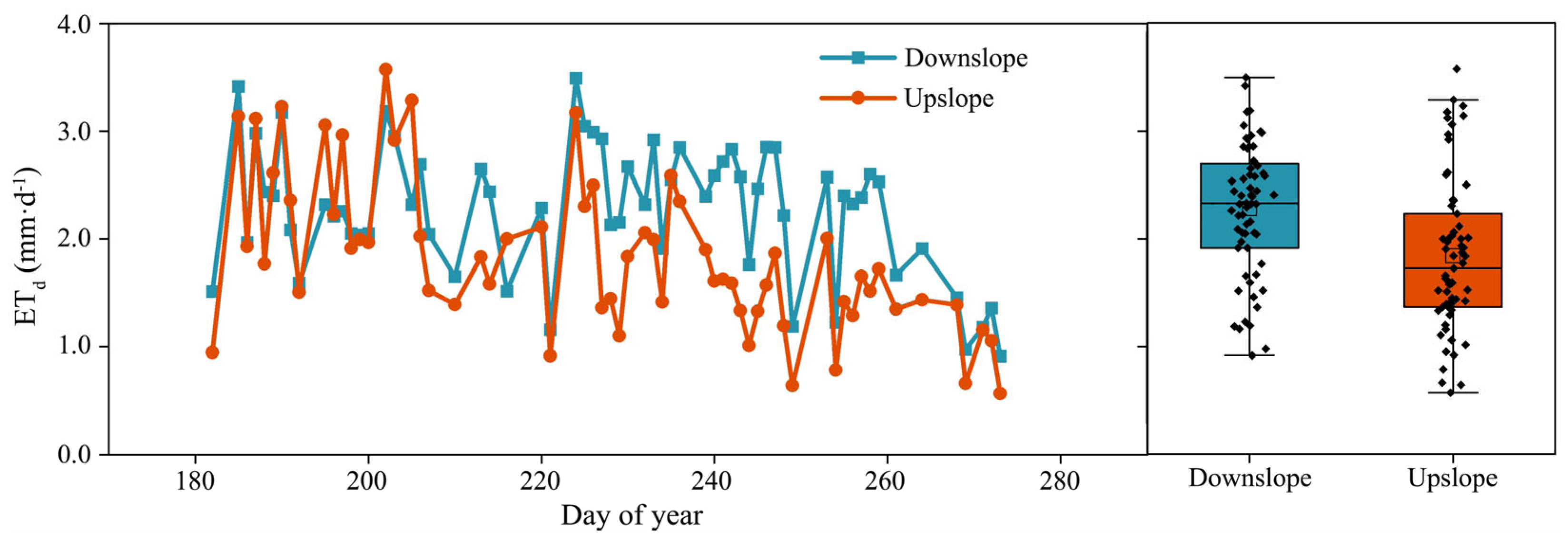
3.2. Variations in ET_d at the Two Slope Positions

Figure 5 shows the variation in daily ET_d at the two slope positions during dry days. The daily ET_d of the two slope positions varied considerably due to variations in environmental conditions. The daily ET_d had means of 2.27 mm·d⁻¹ downslope and 1.84 mm·d⁻¹ upslope but varied widely within the ranges of 0.91–3.49 mm·d⁻¹ and 0.57–3.57 mm·d⁻¹, respectively. The differences in ET_d between the two slope positions varied among the months, with ET_d essentially being the same between the two slope positions in July and with ET_d being greater downslope than upslope in August and September because of the lower soil moisture content. The variation in the difference in ET_d between the two slope positions may be the result of a combination of meteorology and soil moisture.

3.3. Impact of the Main Factors Controlling Evapotranspiration

The responses of ET_d to R_s, VPD, and SWC are shown in Figure 6. As R_s increased, ET_d increased rapidly and then slowly, indicating a logarithmic functional relationship (ET_d = a₁ × ln(R_s) − b₁). As the VPD increased, ET_d increased rapidly and then gradually levelled off, showing a saturated exponential relationship (ET_d = a₂ + b₂ × (1 − EXP(−c₂ × VPD))). As the SWC increased, the ET_d increased rapidly, showing a linear relationship (ET_d = a₃ × SWC + b₃).

A multifactor-influenced ET_d model structure (ET_d = (a₁ × ln(R_s) − b₁) ×(a₂ + b₂ × (1 − EXP(−c₂ × VPD))) ×(a₃ × SWC + b₃)) was established by coupling the above single-factor response relationships through the J-S equation and then fitting them with measured data to obtain a parametric ET_d model (

Table 4. Parameter values for the developed ET_d model.

Model Parameters	Value	P	R2	NSE	n
a1	2.479	<0.01	0.68	0.68	126
b1	6.880
a2	0.058
b2	3.188
c2	0.002
a3	16.641
b3	2.136

). The R² and NSE of the developed model were 0.68 and 0.68, respectively (Figure 7), indicating that the model had good simulation performance and could better reflect the impacts of R_s, VPD, and SWC.

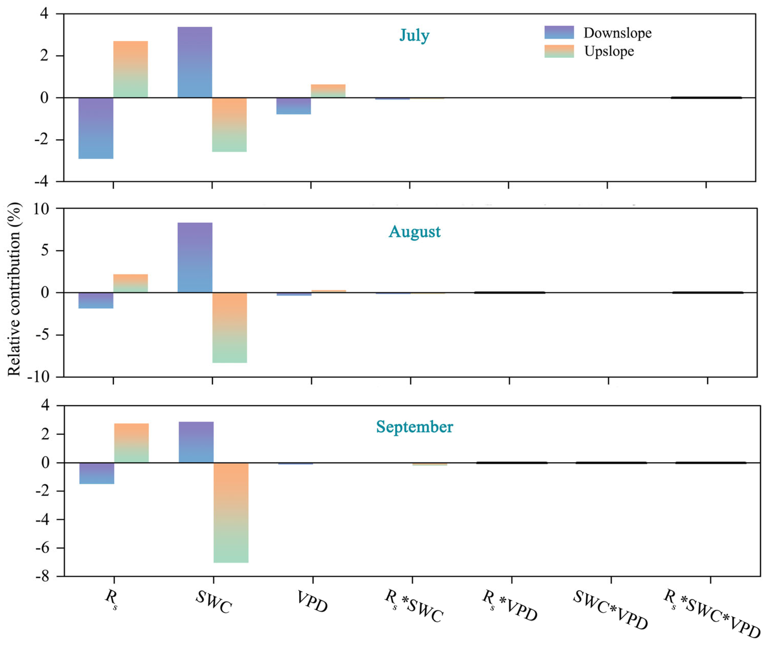
3.4. Relative Contributions of the Main Controlling Factors at the Two Slope Positions

The relative contributions of R_s, VPD, SWC, and their interaction to ET_d at the two slope positions compared with the reference ET_d under the slope-averaged meteorological and soil moisture conditions are shown in Figure 8. R_s had a clear limiting effect on ET_d downslope in different months, with a mean contribution of −2.1%. The largest limiting effect occurred in July, with a contribution of −2.9%. Conversely, R_s had a clear promotional effect on ET_d at the upslope position in different months, with a mean contribution of 2.6%. The greatest promotional effect occurred in September, with a contribution of 2.8%. SWC had an obvious promotional effect on ET_d downslope in different months, with a mean contribution of 4.8%. The greatest promotional effect occurred in September, with a contribution of 8.3%. Conversely, SWC had an obvious limiting effect on ET_d upslope in different months, with a mean contribution of −6.0%. The largest limiting effect occurred in July, with a contribution of −8.3%. The VPD had slight limiting and promotional effects on ET_d in July, with contributions of −0.9 and 0.6 at the downslope and upslope positions, respectively, and had no discernible effect on ET_d in August and September. The interactions between the factors had no discernible effect on ET_d at the two slope positions. Overall, R_s and SWC were the dominant factors contributing to the differences in ET_d between the slope positions, with SWC being the main limiting factor for ET_d at the upslope position and R_s for ET_d at the downslope position.

4. Discussion

4.1. General Response of Evapotranspiration to the Main Controlling Factors

Solar radiation reflects the amount of energy available for evapotranspiration; VPD affects the stomatal resistance of tree transpiration and the soil surface resistance of soil evaporation; therefore, these are critical atmospheric factors affecting evapotranspiration. Evapotranspiration mainly comprises canopy transpiration and forest floor evapotranspiration. In this study, these accounted for 45.9% (45.4%) and 54.1% (54.6%), respectively, at the downslope (upslope) position (see Table S1). Solar radiation and VPD influence the total evapotranspiration process by regulating these two key components. Du et al. [36] reported that solar radiation was the strongest determinant of evapotranspiration. Typically, evapotranspiration varies linearly or nonlinearly with increasing solar radiation [2,28]. In our study, ET_d had a logarithmic relationship with R_s. In water-limited areas, the rate of increase in forest floor evapotranspiration (or soil evaporation) decreases as the atmospheric evaporative demand continues to increase due to limited soil moisture [37]; additionally, many tree species can take some photoprotective measures (such as reducing the stomatal aperture) to prevent damage to the photosynthetic apparatus from excessive light energy, resulting in a reduction in tree transpiration, which was also found in our previous study [30]. This phenomenon may explain why the increase in ET_d was slower at higher R_s. A relatively high VPD indicates that the atmospheric water potential is high and that evapotranspiration of water from the soil and trees is fast and strong [38]; however, trees, especially those growing in water-limited areas, tend to adapt to high VPD conditions by adjusting stomatal conductance to prevent excessive water loss [37,39]. In line with these findings, we observed an asymptotic stabilization of canopy transpiration with increasing VPD (see Figure S1), which suggests that the studied larch forest has effective stomatal control. This can explain the response relationship observed in this study, where ET_d first increased but then tended to saturate with increasing VPD. The impact of the SWC on evapotranspiration depends on the soil moisture [17]. Previous studies have found a near-linear relationship between canopy transpiration and SWC under soil moisture deficit conditions [3,30]. During our study period, which was characterized by low rainfall and relatively dry soils, we observed a significant linear relationship between canopy transpiration and SWC (see Figure S1). Consequently, ET_d was found to depend linearly on soil moisture availability.

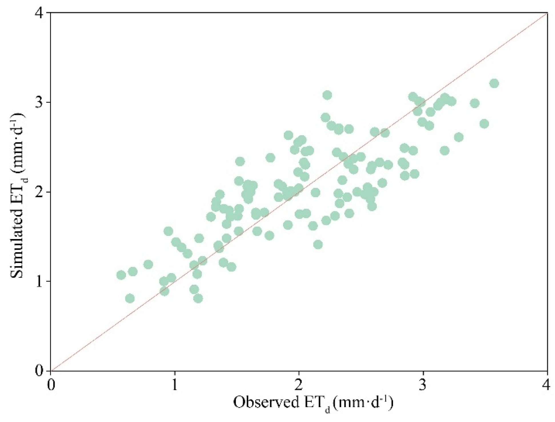
4.2. Evapotranspiration Model Coupled with the Main Controlling Factors

A large variety of evapotranspiration models have been developed and can be roughly divided into remote sensing-based ET models, analytical ET models, and empirical ET models [40], which play important roles in practical applications. The research objectives largely determine the model structure and type. Empirical models play a unique role in quantifying factor contributions, as they include the effects of dominant factors. Although several empirical ET models have been developed on the basis of the mathematical relationships between ET and its controlling factors [28,41,42], their practical application is often limited by coarse temporal resolution (e.g., monthly estimates) and spatial scales at the stand or regional level. Furthermore, the relationships between ET components and environmental drivers can vary significantly at different spatiotemporal scales. For example, Tsuruta et al. [2] showed that evapotranspiration exhibits a nonlinear relationship with control factors (e.g., VPD) on a daily scale, whereas a linear relationship is observed on an annual scale. These scale-dependent dynamics necessitate multi-scale ET modelling due to the fact that the mechanisms of the scale effects in hydrology remain unresolved. Accordingly, we developed an ET_d model that explicitly simulates spatiotemporal variations in ET_d along hillslopes. Compared to existing models, our new model is more applicable at the hillslope scale because it captures finer temporal and broader spatial scales while maintaining model simplicity (only seven parameters) and accuracy.

Atmospheric factors and soil moisture are essential input variables for developing evapotranspiration models. Solar radiation and VPD are well known as the main atmospheric factors influencing evapotranspiration and its components, and PET has often been used in previous studies to adequately reflect the impact of atmospheric conditions [43,44]; however, on hillslopes, each atmospheric factor has a diverse pattern of variation and thus a different contribution to variations in evapotranspiration. To specify the dominant atmospheric factor, multiple potential atmospheric factors need to be considered in ET model construction at the hillslope scale. In this study, an ET_d model combining solar radiation, VPD, and SWC was developed to explain 68% of the variation in ET_d, whereas only 63% of the variation in ET_d could be explained if the model was established on the basis of PET and SWC (ET_d = (0.427 × ln(PET) + 0.442) × (6.167 × SWC + 1.106)), suggesting that the newly developed ET_d model more accurately reflects the effects of meteorological differences on evapotranspiration on hillslopes.

Previous studies have shown that canopy structure (e.g., LAI) has a critical effect on evapotranspiration [45]. In this study, the LAI varied little over the study period at two slope positions, with coefficients of variation ranging from 10 to 13%; additionally, introducing the impact of the LAI did not further improve the model accuracy; therefore, the effect of the LAI was not considered. Although the newly developed ET_d model considers the impact of dominant environmental factors, the model explains only 68% of the variation in ET_d, which may be related to the fact that the model does not consider the influence of biological factors. The dynamics of the coupling between the root system and soil moisture and the regulation of canopy stomata are important biological factors affecting forest transpiration, and the vertical distribution of the root system and its coupling with soil moisture determine the water use strategy of vegetation at different soil depths [46]. As a key parameter of stomatal movement, canopy conductance plays a decisive role in the regulation of transpiration [47], and preliminary observations of canopy conductance on the hillslope in the present study revealed slope differences (unpublished data), which to some extent influence the spatiotemporal variation in transpiration. Additionally, previous studies reported that soil temperature is an important factor affecting forest floor evapotranspiration or soil evaporation [48,49] and thus may have an important influence on forest evapotranspiration. Thus, future studies should explore the influence of additional new factors, with particular emphasis on investigating biological control to evapotranspiration, such as root water uptake strategies and canopy stomatal behaviour, to better understand the mechanism of evapotranspiration at the hillslope scale. Notably, this study developed a site-specific model primarily for quantifying the differential impacts of key factors at two slope positions on evapotranspiration, rather than creating a universal predictive tool applicable across diverse environments. For reliable predictions and regional applications under varying environments, long-term observations across diverse hillslopes are essential for understanding evapotranspiration mechanisms and developing generalizable models.

4.3. Slope Differences and Contributions of Factors to Evapotranspiration

Slope differences in evapotranspiration and its components have been reported; for example, Zhang et al. [50] reported higher ET at upslope positions than at downslope positions. Metzen et al. [51] reported that the difference in transpiration along slopes varied with slope position; transpiration was clearly greater at the downslope position than at the upslope position on a sunny hillslope, and there was no discernible difference in transpiration between the upslope and downslope positions on a shady hillslope. In our study, ET_d was greater at the downslope position than at the upslope position. Numerous studies have shown that the main factors (e.g., solar radiation, PET, and soil moisture) controlling evapotranspiration have clear spatial and temporal variations on hillslopes [52,53]; therefore, diverse reported results on slope differences in evapotranspiration and its components are related mainly to the characteristics of the distribution of the slope microenvironment (e.g., meteorology and soil moisture). This is confirmed by recent studies of evapotranspiration and its components at the hillslope scale; e.g., Liu et al. [54] reported that the attenuation of soil moisture led to lower transpiration at the upslope position than at the downslope position, and Zhang et al. [50] reported that a lower PET due to mountain shading was the main determinant of the lower evapotranspiration at the downslope position than at the upslope position. The relative contribution of each main factor to ET_d was quantified in this study using a newly developed ET_d model, which suggested that solar radiation and soil moisture were the main factors contributing to slope differences in ET_d. Although ET_d was higher at the downslope position, it was still limited by energy availability because the solar radiation was much lower at the downslope position than at the upslope position because of the shading effect of the mountains. The lower soil moisture led to a lower ET_d upslope, and thus, the ET_d upslope was limited by water availability. Soil moisture tends to be transported downslope by gravity, and combined with higher potential evapotranspiration upslope, soil moisture is relatively low upslope, which has been reported in previous studies [26,54]. Furthermore, our study confirms that there are differences in forest evapotranspiration on hillslopes according to slope, and the sites where solar radiation and soil moisture are close to the average slope should be used as representative sample sites for observing evapotranspiration when slope-scale evapotranspiration estimates are conducted.

The primary objective of this study was to develop a methodological framework for quantifying the contributions of environmental factors to variations in evapotranspiration across different slope positions. The three-month data set was used to validate the proposed methodology. Notably, although the methodological framework is universally applicable, the specific quantitative relationships (i.e., the mathematical expressions between evapotranspiration and environmental factors) are slope-specific and cannot be transferred directly to other hillslopes. For future applications to contribution analyses on other hillslopes, quantitative models of evapotranspiration and environmental factors will need to be reconstructed for each target hillslope according to our framework. Additionally, given potential interannual variations in the slope pattern of environmental conditions (particularly soil moisture), future research should incorporate representative hydrological years (normal, wet, and dry years) to systematically investigate factor contribution mechanisms to provide theoretical support for the accurate prediction of evapotranspiration at the hillslope scale.

5. Conclusions

ET_d differed between the two slope positions, and this difference varied by month, with no discernible differences in July but clear differences in August and September. The ET_d model developed by coupling the impacts of solar radiation, VPD, and soil moisture effectively elucidated the spatiotemporal variation mechanisms driven by environmental factors. The independent and interactive effects of environmental drivers on ET_d between two slope positions were quantified using the newly proposed methodology, and solar radiation and soil moisture were the determinants controlling ET_d variations across slope positions, with downslope factors primarily regulated by solar radiation and upslope factors constrained by soil moisture. Our work reveals that variations in environmental conditions caused by slope topography dominate slope differences in ET_d, which may provide theoretical guidance for the future development of methods or models to accurately assess forest evapotranspiration at the scale of individual hillslopes.

References

1. Wang, R.; Gentine, P.; Yin, J.B.; Chen, L.J.; Chen, J.Y.; Li, L.H. Long-term relative decline in evapotranspiration with increasing runoff on fractional land surfaces. Hydrol. Earth Syst. Sci. 2021, 25, 3805–3818. [Google Scholar] [CrossRef]
2. Tsuruta, K.; Kosugi, Y.; Takanashi, S.; Tani, M. Inter-annual variations and factors controlling evapotranspiration in a temperate Japanese cypress forest. Hydrol. Process. 2016, 30, 5012–5026. [Google Scholar] [CrossRef]
3. Liu, Z.B.; Yu, S.P.; Xu, L.H.; Wang, Y.H.; Yu, P.T.; Chao, Y. Differentiated responses of daytime and nighttime sap flow to soil water deficit in a larch plantation in Northwest China. Agric. Water Manag. 2023, 289, 108540. [Google Scholar] [CrossRef]
4. Komatsu, H.; Kume, T. Modeling of evapotranspiration changes with forest management practices: A genealogical review. J. Hydrol. 2020, 585, 124835. [Google Scholar] [CrossRef]
5. Fabiani, G.; Klaus, J.; Penna, D. The influence of hillslope topography on beech water use: A comparative study in two different climates. Hydrol. Earth Syst. Sci. 2024, 28, 2683–2703. [Google Scholar] [CrossRef]
6. Mitchell, P.J.; Benyon, R.G.; Lane, P.N. Responses of evapotranspiration at different topographic positions and catchment water balance following a pronounced drought in a mixed species eucalypt forest, Australia. J. Hydrol. 2012, 440, 62–74. [Google Scholar] [CrossRef]
7. Tsuruta, K.; Yamamoto, H.; Kosugi, Y.; Makita, N.; Katsuyama, M.; Kosugi, K.; Tani, M. Slope position and water use by trees in a headwater catchment dominated by Japanese cypress: Implications for catchment-scale transpiration estimates. Ecohydrology 2020, 13, e2245. [Google Scholar] [CrossRef]
8. Casirati, S.; Conklin, M.H.; Nandi, S.; Safeeq, M. Effect of forest management practices on water balance across a water–energy gradient in the upper Kings River Basin, USA. Ecohydrology 2025, 18, e2753. [Google Scholar] [CrossRef]
9. Bonell, M. Selected challenges in runoff generation research in forests from the hillslope to headwater drainage basin scale. J. Am. Water Resour. As. 1998, 34, 765–785. [Google Scholar] [CrossRef]
10. Wolf, S.; Paul-limoges, E.; Sayler, D.; Kirchner, J.W. Dynamics of evapotranspiration from concurrent above- and below-canopy flux measurements in a montane Sierra Nevada forest. Agric. For. Meteorol. 2024, 346, 109864. [Google Scholar] [CrossRef]
11. Inokoshi, S.; Gomi, T.; Chiu, C.; Onda, Y.; Hashimoto, A.; Zhang, Y.; Saitoh, T.M. A watershed-scale evapotranspiration model considering forest type, stand parameters, and climate factors. For. Ecol. Manag. 2023, 547, 121387. [Google Scholar] [CrossRef]
12. Benyon, R.G.; Doody, T.M. Comparison of interception, forest floor evaporation and transpiration in Pinus radiata and Eucalyptus globulus plantations. Hydrol. Process. 2015, 29, 1173–1187. [Google Scholar] [CrossRef]
13. Zhang, Y.Q.; Peña-Arancibia, J.L.; McVicar, T.R.; Chiew, F.H.; Vaze, J.; Liu, C.M.; Lu, X.J.; Zheng, H.X.; Wang, Y.P.; Liu, Y.Y.; et al. Multi-decadal trends in global terrestrial evapotranspiration and its components. Sci. Rep. 2016, 6, 19124. [Google Scholar] [CrossRef]
14. Wen, R.H.; Qin, M.O.; Jiang, P.; Yang, F.; Liu, B.; Zhu, M.Y.; Fang, Y.; Tian, Y.C.; Shang, B. Vegetation and evapotranspiration responses to increased atmospheric vapor pressure deficit across the global forest. Atmosphere 2024, 15, 408. [Google Scholar] [CrossRef]
15. Zhang, B.Z.; Xu, D.; Liu, Y.; Li, F.S.; Cai, J.B.; Du, L.J. Multi-scale evapotranspiration of summer maize and the controlling meteorological factors in north China. Agric. For. Meteorol. 2016, 216, 1–12. [Google Scholar] [CrossRef]
16. Novick, K.A.; Ficklin, D.L.; Stoy, P.C.; Williams, C.A.; Bohrer, G.; Oishi, A.C.; Papuga, S.A.; Blanken, P.D.; Noormets, A.; Sulman, B.N.; et al. The increasing importance of atmospheric demand for ecosystem water and carbon fluxes. Nat. Clim. Change 2016, 6, 1023–1027. [Google Scholar] [CrossRef]
17. Scott, R.L.; Knowles, J.F.; Nelson, J.A.; Gentine, P.; Li, X.; Barron-Gafford, G.; Bryant, R.; Biederman, J.A. Water availability impacts on evapotranspiration partitioning. Agric. For. Meteorol. 2021, 297, 108251. [Google Scholar] [CrossRef]
18. Jung, M.; Reichstein, M.; Ciais, P.; Seneviratne, S.I.; Sheffield, J.; Goulden, M.L.; Bonan, G.; Cescatti, A.; Chen, J.; de Jeu, R.; et al. Recent decline in the global land evapotranspiration trend due to limited moisture supply. Nature 2010, 467, 951–954. [Google Scholar] [CrossRef]
19. A, Y.L.; Wang, G.Q.; Liu, T.X.; Xue, B.L.; Kuczera, G. Spatial variation of correlations between vertical soil water and evapotranspiration and their controlling factors in a semi-arid region. J. Hydrol. 2019, 574, 53–63. [Google Scholar] [CrossRef]
20. Donaldson, A.; Dralle, D.; Barling, N.; Callahan, R.P.; Loik, M.E.; Zimmer, M. Aspect differences in vegetation type drive higher evapotranspiration on a pole-facing slope in a California Oak Savanna. J. Geophys. Res.-Biogeo. 2024, 129, e2024JG008054. [Google Scholar] [CrossRef]
21. Lin, P.F.; Zhao, P.; Ma, J.; Yang, J.J.; Zhu, X.; Tian, Q.Y.; Du, J.; Chen, L.F.; He, Z.B. Modulation of evapotranspiration and stream runoff by weathered bedrock in arid and semi-arid mountains. Sci. Total Environ. 2024, 930, 172847. [Google Scholar] [CrossRef]
22. Wang, H.L.; Guan, H.D.; Xu, X.; Gao, L.M.; Gutiérrez-Jurado, H.A.; Simmons, G.T.; Simmons, C.T. Topographic regulations on ecohydrological dynamics in a montane forest catchment and the implications for plant adaptation to environment. J. Hydrol. 2024, 637, 131412. [Google Scholar] [CrossRef]
23. Xu, M.J.; An, T.T.; Zheng, Z.Y.; Zhang, T.; Zhang, Y.J.; Yu, G.R. Variability in evapotranspiration shifts from meteorological to biological control under wet versus drought conditions in an alpine meadow. J. Plant Ecol. 2022, 15, 921–932. [Google Scholar] [CrossRef]
24. Li, X.; Xu, X.; Tian, W.; Tian, J.; He, C. Contribution of climate change and vegetation restoration to interannual variability of evapotranspiration in the agro-pastoral ecotone in northern China. Ecol. Indic. 2023, 154, 110485. [Google Scholar] [CrossRef]
25. da Silva, J.B.; Valle, L.C.G., Jr.; Faria, T.O.; Marques, J.B.; Dalmagro, H.J.; Nogueira, J.S.; Vourlitis, G.L.; Rodrigues, T.R. Temporal variability in evapotranspiration and energy partitioning over a seasonally flooded scrub forest of the Brazilian Pantanal. Agric. For. Meteorol. 2021, 308, 108559. [Google Scholar] [CrossRef]
26. Fabiani, G.; Schoppach, R.; Penna, D.; Klaus, J. Transpiration patterns and water use strategies of beech and oak trees along a hillslope. Ecohydrology 2022, 15, e2382. [Google Scholar] [CrossRef]
27. Li, H.X.; Zhou, H.Y.; Wei, X.H.; Liang, Z.X.; Liu, S.J.; Huang, J.G. The impact of slope positions on stand transpiration of a Zenia insignis plantation in North Guangdong Province, South China. Desalin. Water Treat. 2021, 219, 164–171. [Google Scholar] [CrossRef]
28. Yang, F.L.; Zhou, G.S. Characteristics and modeling of evapotranspiration over a temperate desert steppe in Inner Mongolia, China. J. Hydrol. 2011, 396, 139–147. [Google Scholar] [CrossRef]
29. Blöschl, G.; Sivapalan, M. Scale issues in hydrological modelling: A review. Hydrol. Process. 1995, 9, 251–290. [Google Scholar] [CrossRef]
30. Liu, Z.B.; Yu, S.P.; Xu, L.H.; Wang, Y.H.; Wang, M.F.; Yu, P.T. Spatiotemporal variations in sap flow in a larch plantation: Sampling size for stand scale estimates. J. Forestry Res. 2024, 35, 139. [Google Scholar] [CrossRef]
31. Han, C.; Chen, N.; Zhang, C.K.; Liu, Y.J.; Khan, S.; Lu, K.L.; Li, Y.G.; Dong, X.X.; Zhao, C.M. Sap flow and responses to meteorological about the Larix principis-rupprechtii plantation in Gansu Xinlong mountain, northwestern China. For. Ecol. Manag. 2019, 451, 117519. [Google Scholar] [CrossRef]
32. Flo, V.; Martinez-Vilalta, J.; Steppe, K.; Schuldt, B.; Poyatos, R. A synthesis of bias and uncertainty in sap flow methods. Agric. For. Meteorol. 2019, 271, 362–374. [Google Scholar] [CrossRef]
33. Jiao, L.; Lu, N.; Fang, W.; Li, Z.; Wang, J.; Jin, Z. Determining the independent impact of soil water on forest transpiration: A case study of a black locust plantation in the Loess Plateau, China. J. Hydrol. 2019, 572, 671–681. [Google Scholar] [CrossRef]
34. Schmidt, U.; Thöni, H.; Kaupenjohann, M. Using a boundary line approach to analyze N2O flux data from agricultural soils. Nutr. Cycl. Agroecosys. 2000, 57, 119–129. [Google Scholar] [CrossRef]
35. Waseem, M.; Mani, N.; Andiego, G.; Usman, M. A review of criteria of fit for hydrological models. Int. Res. J. Eng. Technol. 2017, 4, 1765–1772. [Google Scholar]
36. Du, M.C.; Zhang, J.Y.; Wang, Y.; Liu, H.W.; Wang, Z.L.; Liu, C.S.; Yang, Q.L.; Hu, Y.S.; Bao, Z.X.; Liu, Y.L.; et al. Evaluating the contribution of different environmental drivers to changes in evapotranspiration and soil moisture, a case study of the Wudaogou Experimental Station. J. Contam. Hydrol. 2021, 243, 103912. [Google Scholar] [CrossRef]
37. Han, X.S.; Wang, Y.H.; Li, Z.H.; Wang, Y.B.; Yu, P.T.; Xiong, W. Daily forest floor evapotranspiration of Larix principis-rupprechtii plantation and its influencing factors in the semi-arid area of Liupan Mountains. Sci. Silvae Sin. 2019, 55, 11–21. (In Chinese) [Google Scholar]
38. da Silva, I.W.; Marques, T.V.; Urbano, S.A.; Mendes, K.R.; Oliveira, A.C.C.; Nascimento, F.D.S.; de Morais, L.F.; Pereira, W.D.S.; Mutti, P.R.; Neto, J.V.E.; et al. Meteorological and biophysical controls of evapotranspiration in tropical grazed pasture under rainfed conditions. Agr. Water Manag. 2024, 299, 108884. [Google Scholar] [CrossRef]
39. Broughton, K.J.; Conaty, W.C. Understanding and exploiting transpiration response to vapor pressure deficit for water limited environments. Front. Plant. Sci. 2022, 13, 893994. [Google Scholar] [CrossRef]
40. Ghiat, I.; Mackey, H.R.; Al-Ansari, T. A review of evapotranspiration measurement models, techniques and methods for open and closed agricultural field applications. Water 2021, 13, 2523. [Google Scholar] [CrossRef]
41. Bunting, D.P.; Kurc, S.A.; Glenn, E.P.; Nagler, P.L.; Scott, R.L. Insights for empirically modeling evapotranspiration influenced by riparian and upland vegetation in semiarid regions. J. Arid Environ. 2014, 111, 42–52. [Google Scholar] [CrossRef]
42. Sawano, S.; Hotta, N.; Tanaka, N.; Tsuboyama, Y.; Suzuki, M. Development of a simple forest evapotranspiration model using a process-oriented model as a reference to parameterize data from a wide range of environmental conditions. Ecol. Model. 2015, 309–310, 93–109. [Google Scholar] [CrossRef]
43. Marques, T.V.; Mendes, K.; Mutti, P.; Medeiros, S.; Silva, L.; Perez-Marin, A.M.; Campos, S.; Lúcio, P.S.; Lima, K.; dos Reis, J.; et al. Environmental and biophysical controls of evapotranspiration from seasonally dry tropical forests (Caatinga) in the Brazilian semiarid. Agric. For. Meteorol. 2020, 287, 107957. [Google Scholar] [CrossRef]
44. Niu, X.D.; Chen, Z.C.; Pang, Y.; Niu, B.L.; Yan, C.Y.; Liu, S.R. Environmental and biological controls on the interannual variations of evapotranspiration in a natural oak forest. Agric. For. Meteorol. 2024, 349, 109969. [Google Scholar] [CrossRef]
45. Liu, C.; Sun, G.; McNulty, S.G.; Kang, S. An improved evapotranspiration model for an apple orchard in northwestern China. Trans. ASABE 2015, 58, 1253–1264. [Google Scholar]
46. Amenu, G.G.; Kumar, P. A model for hydraulic redistribution incorporating coupled soil-root moisture transport. Hydrol. Earth Syst. Sci. 2008, 12, 55–74. [Google Scholar] [CrossRef]
47. Song, L.N.; Zhu, J.J.; Zheng, X.; Wang, K.; Lü, L.Y.; Zhang, X.L.; Hao, G.Y. Transpiration and canopy conductance dynamics of Pinus sylvestris var. mongolica in its natural range and in an introduced region in the sandy plains of Northern China. Agric. For. Meteorol. 2020, 281, 107830. [Google Scholar] [CrossRef]
48. Fetzer, T.; Vanderborght, J.; Mosthaf, K.; Smits, K.M.; Helmig, R. Heat and water transport in soils and across the soil-atmosphere interface: 2. Numerical analysis. Water Resour. Res. 2017, 53, 1080–1100. [Google Scholar] [CrossRef]
49. Di, N.; Wang, Y.; Clothier, B.; Liu, Y.; Jia, L.M.; Xi, B.Y.; Shi, H.X. Modeling soil evaporation and the response of the crop coefficient to leaf area index in mature Populus tomentosa plantations growing under different soil water availabilities. Agric. For. Meteorol. 2019, 264, 125–137. [Google Scholar] [CrossRef]
50. Zhang, Y.K.; Huang, M.B. Spatial variability and temporal stability of actual evapotranspiration on a hillslope of the Chinese Loess Plateau. J. Arid Land 2021, 13, 189–204. [Google Scholar] [CrossRef]
51. Metzen, D.; Sheridan, G.J.; Benyon, R.G.; Bolstad, P.V.; Griebel, A.; Lane, P.N. Spatio-temporal transpiration patterns reflect vegetation structure in complex upland terrain. Sci. Total Environ. 2019, 694, 133551. [Google Scholar] [CrossRef]
52. Lu, S.G.; Liu, M.X.; Yi, J.; Zhang, H.L.; Wan, J.H. Responses of soil moisture at different topographic positions to rainfall events along a steep subtropical forested hillslope. Hydrol. Process. 2024, 38, e15164. [Google Scholar] [CrossRef]
53. Renner, M.; Hassler, S.K.; Blume, T.; Weiler, M.; Hildebrandt, A.; Guderle, M.; Schymanski, S.J.; Kleidon, A. Dominant controls of transpiration along a hillslope transect inferred from ecohydrological measurements and thermodynamic limits. Hydrol. Earth Syst. Sci. 2016, 20, 2063–2083. [Google Scholar] [CrossRef]
54. Liu, W.N.; Nie, Y.P.; Luo, Z.D.; Wang, Z.Y.; Huang, L.; He, F.; Chen, H.S. Transpiration rates decline under limited moisture supply along hillslopes in a humid karst terrain. Sci. Total Environ. 2023, 894, 164977. [Google Scholar] [CrossRef] [PubMed]
Figure 1. Schematic representation of the location of the study sample plots on the hillslope.
Forests 16 01035 g001
Figure 2. The structure of microlysimeters.
Forests 16 01035 g002
Figure 3. Flowchart of the methodology for determining the contributions of the dominant factors to evapotranspiration at different slope positions.
Forests 16 01035 g003
Figure 4. Temporal dynamics of solar radiation (Rs), vapor pressure deficit (VPD), and the soil water content (SWC) and their differences at the two slope positions.
Forests 16 01035 g004
Figure 5. Temporal dynamics of evapotranspiration on dry days (ETd) at the two slope positions.
Forests 16 01035 g005
Figure 6. The response of ETd to the Rs, VPD, and SWC.
Forests 16 01035 g006
Figure 7. Comparison of model simulated ETd values with observed ETd values.
Forests 16 01035 g007
Figure 8. The relative contributions of Rs, VPD, SWC, and their interaction to ETd at the two slope positions.
Forests 16 01035 g008