From Regression to Machine Learning: Modeling Height–Diameter Relationships in Crimean Juniper Stands Without Calibration Overhead

Abstract

Accurate modeling of height–diameter (h–d) relationships is critical for forest inventory and management, particularly in complex forest ecosystems such as natural and pure Crimean juniper (Juniperus excelsa Bieb.) stands. This study evaluates both traditional parametric and modern machine learning (ML) approaches to develop reliable h–d models based on 2135 sample trees measured in southern Türkiye. The modeling approaches include fixed-effects (FE), mixed-effects (ME), three quantile regression (QR) models based on three, five, and nine quantile levels, and non-parametric ML methods: shallow multilayer perceptron (S_MLP), extreme gradient boost (XGBoost), and random forest (RF). According to the assessment metrics for the fitting and test datasets, the XGBoost modeling approach achieved the most accurate performance. For the fitting dataset, it achieved root mean square error values of 1.11 m and 1.21 m. For the test dataset, the corresponding error values were 1.16 m and 1.24 m, resulting in the highest accuracy among all models, closely followed by the RF and S_MLP models. A key practical advantage of ML approaches is that they do not depend on calibration scenarios, meaning they can operate without the need for preliminary parameter configuration. In contrast, the ME model showed the highest accuracy among the parametric methods when calibration was applied. In this case, when applying ME models, the study recommends calibrating the model by measuring four randomly selected trees per plot to balance prediction accuracy and field sampling effort.

1. Introduction

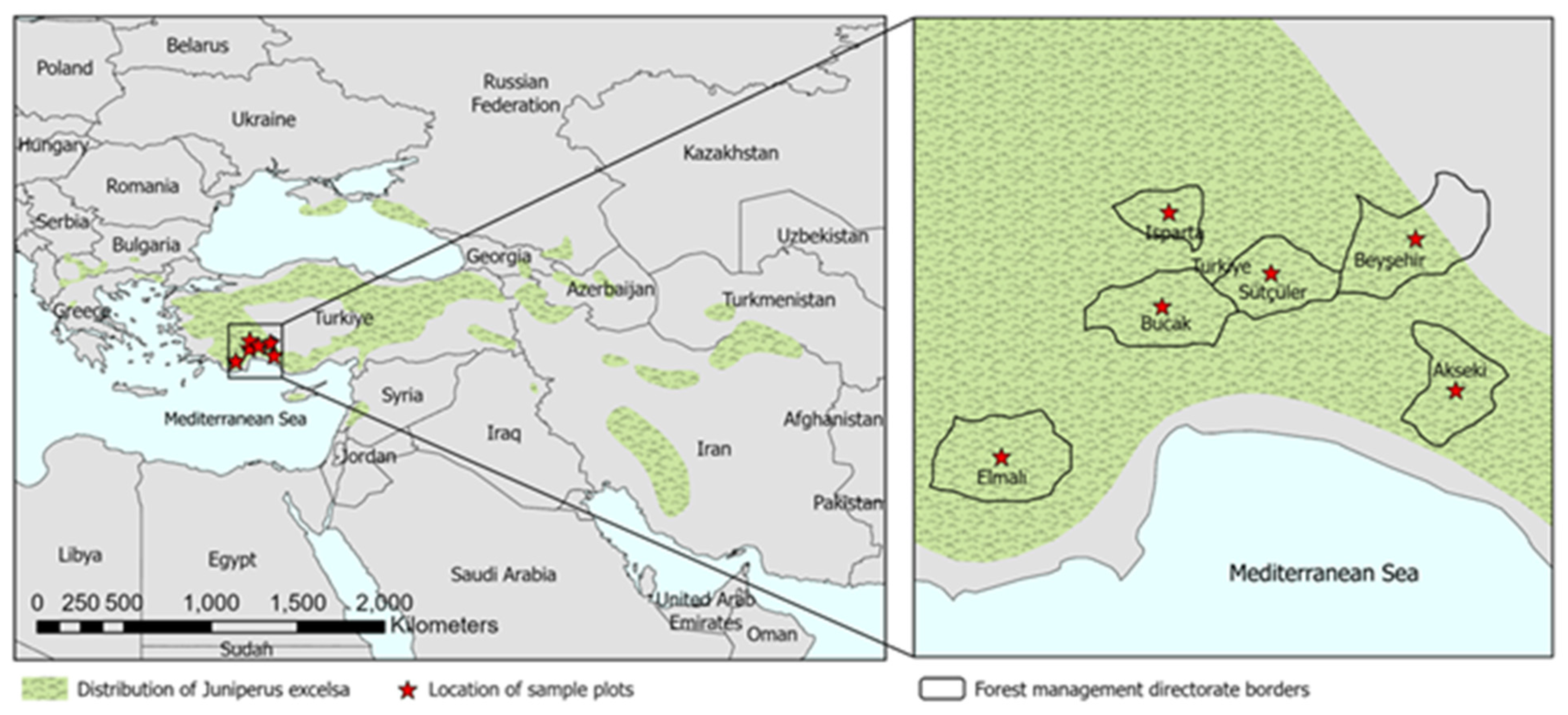
Juniperus is an economically and ecologically significant species in Türkiye, covering 1.6 million ha with a standing volume of 32.6 million m³ [1]. Juniper species are distributed commonly in the Taurus Mountains. Six juniper species naturally grow in Türkiye; among them, Crimean juniper (Juniperus excelsa Bieb.) is the most common and has great economic potential. The most significant distribution area of the species worldwide is Türkiye. Therefore, it offers several environmental benefits, including conserving biodiversity, water, and soil resources. Additionally, it serves as a source of essential oils used in Türkiye’s medical and cosmetics industries.

Recently, Türkiye has adopted a novel approach to strengthen the multifunctional role of forests by developing fundamental management strategies to expand the economic, ecological, and social benefits from forests [2]. Growth and yield prediction models are an integral component of this novel approach to create long-term plans for managing forest ecosystems and enhancing their resilience to climate change.

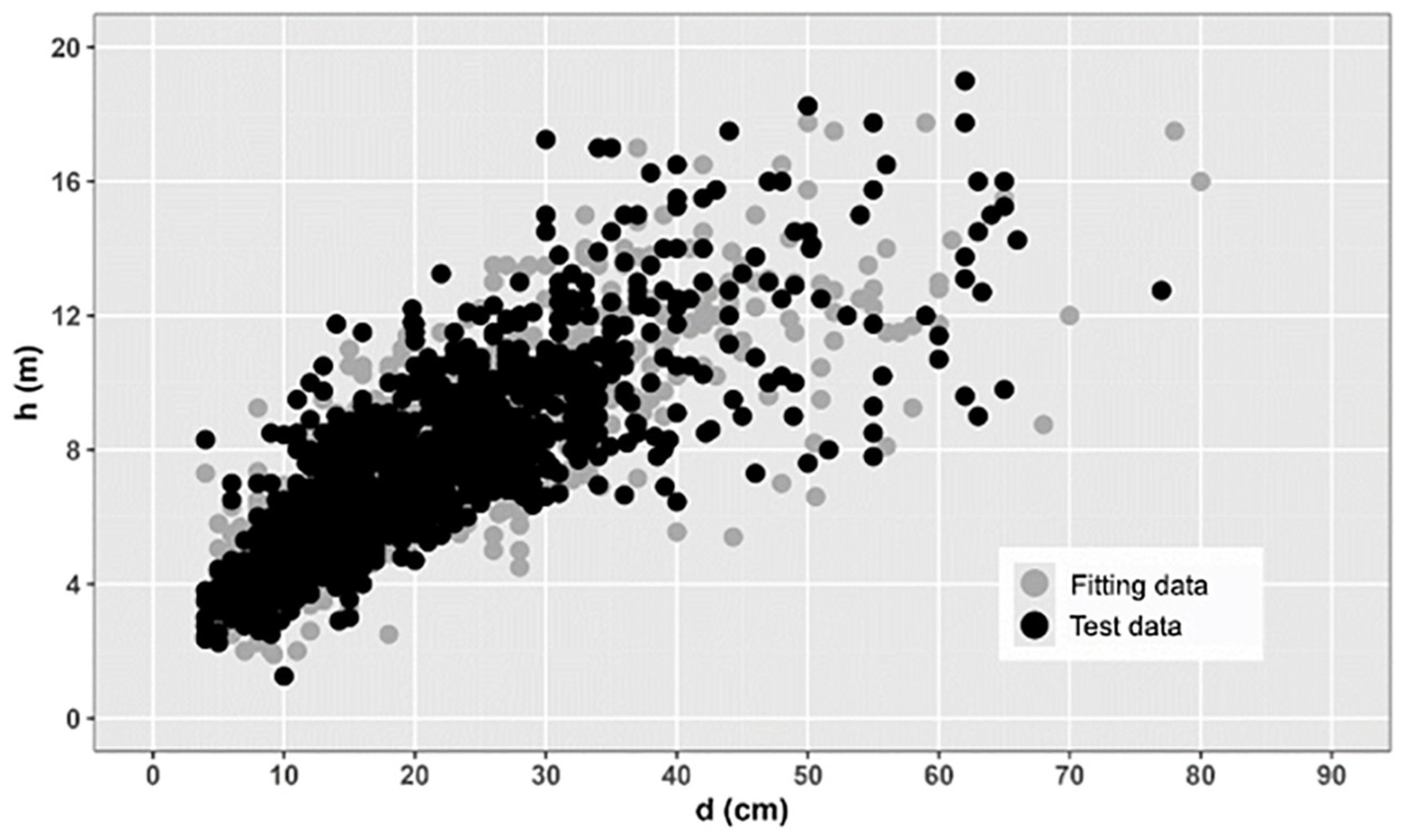
Height–diameter (h–d) models are a key component of growth and yield prediction in forestry. Traditionally, h–d models have relied solely on the diameter at breast height, which was measured 1.3 m above the ground, as the predictor variable for estimating the total height of all of the trees in an area. These models describe the relationship between total tree height (h) and diameter at breast height (d, measured at 1.3 m above ground), which impact forest stands [3], and are widely used in applications such as yield estimation [4,5], stand structure analysis [6], site index determination and dominant height (H₀) estimation [4,7], and carbon budget modeling [8]. Moreover, h–d models are essential for understanding the complex dynamics that define and influence forest stands [3]. Despite their importance, data on the h–d relationship for Crimean juniper is limited, particularly in Türkiye. As noted by Crecente-Campo et al. [9], measuring h is generally more difficult and costly than measuring d.

Numerous h–d models have been developed for plantations and pure, even-aged stands [10,11]. However, a single h–d equation is often inadequate across all stands, as the h–d relationship varies between stands and even within the same stand over time [4]. The conventional solution is to fit a local h–d model for each plot, which requires extensive sampling and increases costs.

To address this, recent studies have explored alternative approaches, such as nonlinear mixed-effects (ME) and quantile regression (QR) models. ME models have been widely applied in h–d modeling efforts [3,12,13,14,15,16,17,18,19,20,21,22,23]. These models include fixed effects, representing population-level trends, and random effects, which account for within-plot variability. ME models are particularly effective at capturing spatial and temporal correlations by specifying covariance structures during parameter estimation [14,20,24]. A key advantage of ME models is their adaptability to local forest conditions. Random effects can be predicted using tree- or stand-level covariates, combined with a small subsample of measured heights and diameters [16,18,23,25]. Traditionally, basic or local h–d models rely solely on diameter at breast height (1.3 m above ground) as a predictor. In contrast, generalized models include additional stand-level variables such as site index, basal area, dominant diameter (D₀), stand age, and H₀ [13,18,26]. Some studies have shown that ME models can accurately capture h–d variability without incorporating additional stand-level predictors [13,15,26,27,28,29,30]. Incorporating stand-level random effects in ME models allows them to reflect variability among stands [31,32]. Moreover, calibrating existing ME models requires significantly less sampling than building new basic models, while maintaining comparable accuracy [19,33]. Thus, model calibration offers an efficient and cost-effective means of achieving reliable h–d predictions [29].

QR, originally developed by Koenker and Bassett [34], offers a novel approach for applications in forest inventory. This method evaluates the conditional distribution of dependent variables, examining the influence of estimates across various quantiles. Unlike mean regression estimators, which only consider the conditional mean or central effects of the covariates, this approach provides a more comprehensive analysis. QR has been effectively applied in forestry for tasks such as defining self-thinning boundaries [35,36], modeling maximum crown width [37], and estimating insect infestation spread rates [38]. It has also been used in stem diameter modeling [39], tree h–d relationships [18,22,28,40,41,42], and growth curve development [43]. These studies show that QR equations can model h–d relationships across various quantiles. Similar to ME models, QR can achieve high prediction accuracy when calibrated. By applying dual QR methods with two h–d equations from different quantiles, it is possible to construct a localized h–d equation that passes through a specific point [18,41].

For parameter estimation of ME and QR models, calibration alternatives can be tested by using different sampling patterns and varying sampling sizes within each sample plot. The advantage of different sampling scenarios in the localization of non-linear ME h–d models has been empirically explored in previous studies. Some studies [7,9] suggested that it is better to choose calibration trees among the smallest trees in the sample plots. In contrast, other studies [18] observed that the prediction performance of ME and QR improved with increasing sample size, with significant improvements noted in evaluation statistics for sample sizes of five or less trees.

Modeling the h–d relationship is challenging due to the biological variability of trees across species and locations. In recent decades, machine learning (ML) methods have emerged as effective, non-parametric alternatives to traditional regression models [44,45,46,47,48,49], and are capable of capturing complex data patterns. Neural networks have been successfully applied in various contexts, including Larch plantations using supervised backpropagation [50] and multilayer networks outperforming nonlinear regression for Pinus koraiensis in the Mengjiagang Forest Farm [51]. Karatepe et al. [52] found neural networks superior to fixed- and mixed-effects models for Cedar height estimation, while Ogana and Ercanli [53] also used artificial neural networks (ANNs) effectively in a tropical Nigerian forest with 116 species. Other studies confirmed the superiority of ANNs over nonlinear mixed-effects (NLME) models [54] and explored decision trees, random forests, support vector machines [55], and deep learning for tree height estimation in urban forests [56].

Given the intense research interest in h–d relationships and the need for accurate, reliable h–d models, especially in light of the limited modeling studies on Crimean juniper and considering that the potential of ML methods in this context remains underexplored, three ML approaches were selected for investigation and comparison with the fixed-effects (FE), ME, and QR parametric methods to develop robust 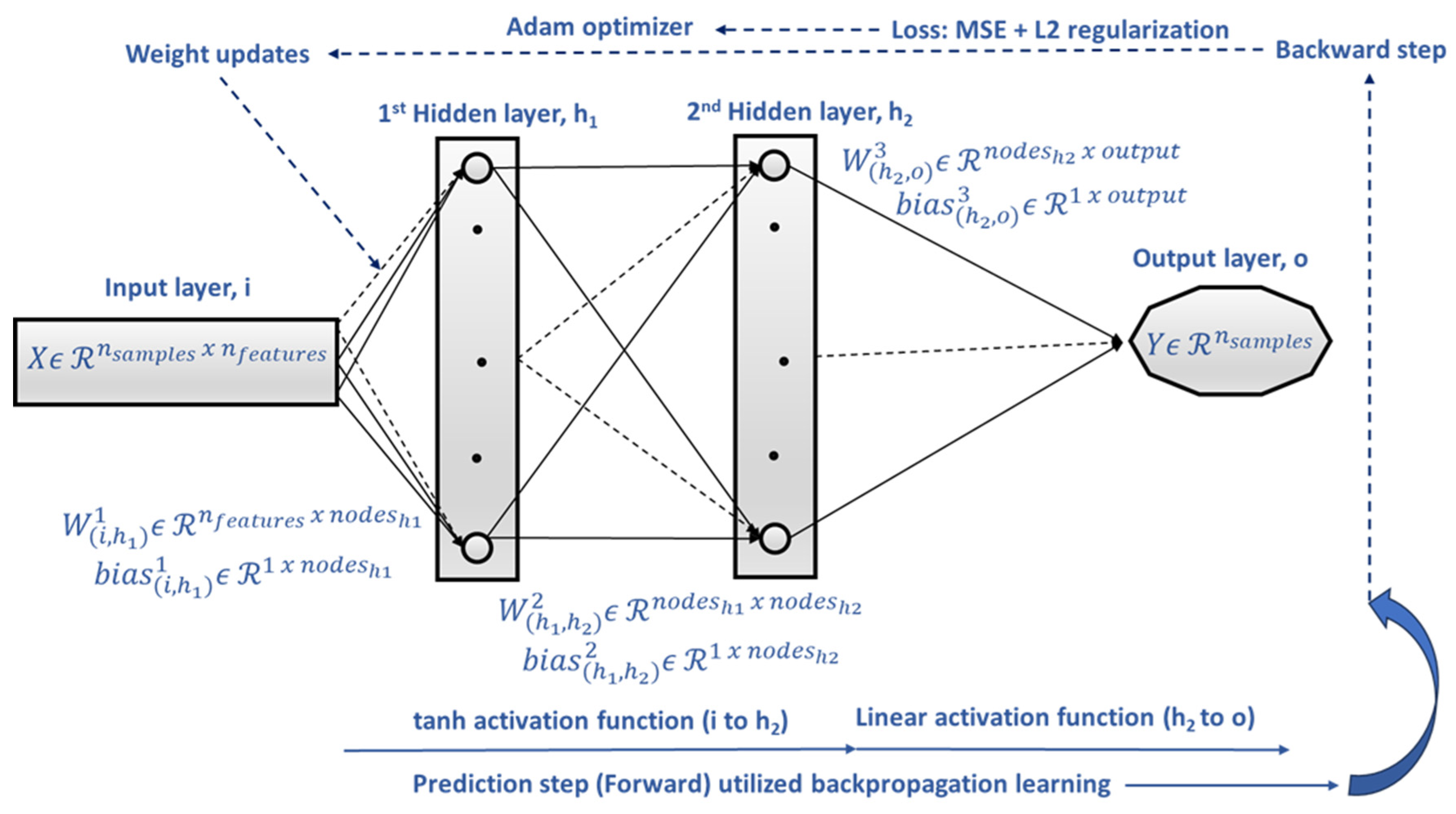h–d models. 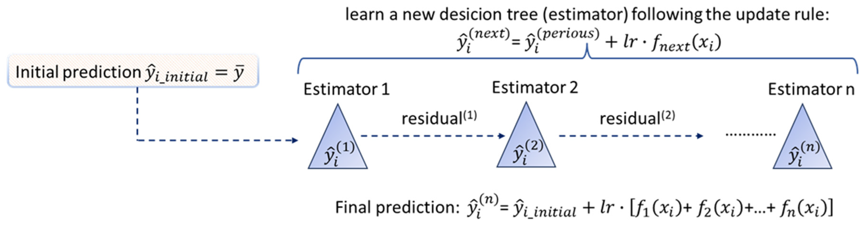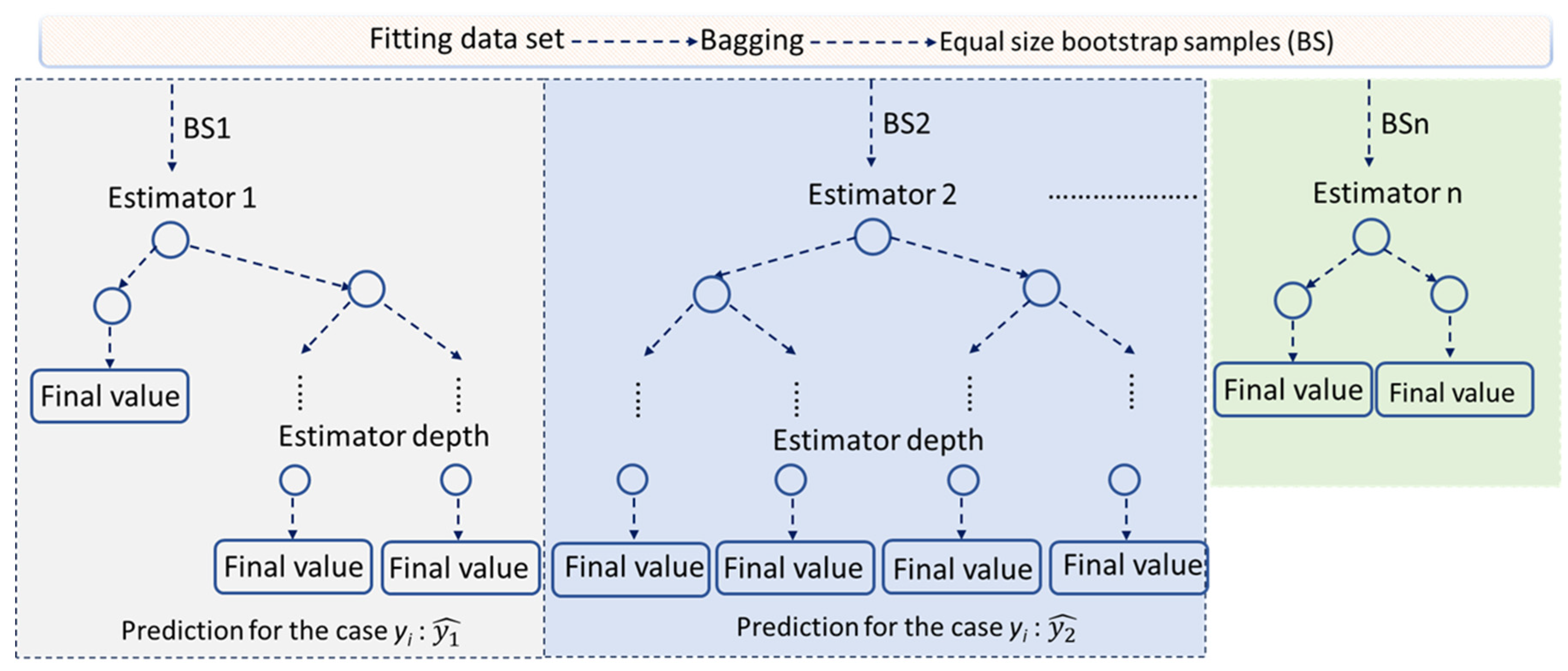Namely, the regression-based non-parametric shallow multilayer perceptron (S_MLP) ANNs, the extreme gradient boost (XGBoost), and the random forest (RF) ML modeling approaches, were selected, on one hand, due to their ability to capture nonlinearity among data, and on the other hand these approaches can effectively handle moderate size datasets, both conditions frequently faced in forest datasets. Furthermore, the selected algorithms bring distinct advantages and limitations [57,58,59,60] due to their differing algorithmic foundations. These characteristics allow the selection of the most appropriate model based on the structure and complexity of the data at hand. In general, the S_MLP approach offers smoothness in the approximation function, and it can effectively learn nonlinear relationships where complexity is present. RF and XGBoost techniques are both considered robust in overfitting by incorporating regularization. However, all approaches, some to a greater extent and some to a lesser extent, require effort in their hyperparameters tuning.

The objectives of this study were as follows: 1. to investigate cutting-edge ML approaches, namely S_MLP, RF, and XGBoost, that leverage diverse algorithmic strategies to develop high-precision h–d models for Juniperus excelsa (Crimean juniper) trees in the Taurus mountains, 2. to develop models that rely on a minimal number of tree variables that are easy to measure in the field, thereby enhancing their practical usefulness in forest management, 3. to conduct a comparative analysis between ML and parametric regression methodologies, 4. to calibrate ME and QR models using different sampling scenarios, and 5. to evaluate these scenarios in order to gain deeper insights into the effectiveness of each modeling approach in predicting tree height.

2. Materials and Methods

2.1. Data

To develop the h–d models, a total of 98 sample plots containing 2135 sample trees were used. A portion of the sample plots used in this study were adopted from the earlier work cited in [15], with data collection conducted before 2013. Additionally, in 2023, thirty-five new sample plots were measured from natural juniper stands in the Isparta and Antalya Regional Directorates of Forestry (Northwest Mediterranean Region) in order to update the previously developed h–d models and to enable the results of the study to represent a wider area. The distribution of sample sites in natural and pure (with more than 90% juniper trees) even-aged juniper stands is shown in Figure 1.

For the variability in the distribution of the species to be reflected, the sample sites were taken from pure and natural juniper stands with different diameter, height, age, and stand density. A subjective sampling approach was used for this purpose. There is no difference in the data collection technique or sampling method applied between the two data groups that were measured at different times.

The diameter at breast height (d, cm) for each tree was determined by averaging two perpendicular measurements taken outside the bark at a height of 1.3 m above ground level, using a digital caliper. Tree height measurements were recorded to the nearest 0.05 m with a Laser-Tech TruPulse device (Laser Technology Inc., Centennial, CO, USA). H₀ and D0 were estimated as the mean height and mean diameter of the 100 largest diameter trees per hectare, respectively. The quadratic mean ${(D}_g)$ and the basal area (G) per hectare were derived by aggregating individual tree measurements within each sample plot. $D_g$ was calculated as $D_g=\sqrt{\sum _{i=1}^n{d}_i^2/n}$, while the G per hectare was calculated as $G=\left(\sum _{i=1}^n{\pi d}_i^2/4\right)·\left(\mathrm{10,000}/A\right)$, where d_i is the diameter at breast height, n is the total number of trees in the plot, and A is the plot area. The above stand variables were estimated at plot level. Plot size ranged from 165 to 3420 m².

Data Division

Of the 98 available plots, 49 were randomly selected for model development, while the remaining 49 were reserved for testing the fitted models. This initial division was consistently applied across both parametric and ML approaches.

For the ML models specifically, to ensure robust and accurate performance while minimizing the risk of underfitting or overfitting, a 10-fold cross-validation procedure was employed on the development (fitting) dataset. In this process, the fitting dataset was repeatedly partitioned into training (90%) and validation (10%) subsets across 10 iterations, as required by the 10-fold cross-validation methodology [61,62].

Based on commonly used h–d regression models in forest modeling research, nine basic nonlinear h–d equations and five nonlinear generalized h–d models that have been previously cited in the literature [19,22,23,63,64,65,66] were selected for this study. These model forms (listed in

Table 1. Base and generalized models tested.

Model	Equation	No.
Power	$h={1.3+\beta }_1{d}^{{\beta }_{2 }}$	(1)
Chapman-Richards	$h=1.3+{\beta }_1{\left(1-exp\left(-{\beta }_{2 }d\right)\right)}^{{\beta }_{3 }}$	(2)
Weibull	$h=1.3+{\beta }_1\left(1-exp\left(-{\beta }_{2 }{d}^{{\beta }_{3 }}\right)\right)$	(3)
Gompertz	$h=1.3+{ \beta }_1\left(exp\left(-{\beta }_{2 } exp\left(-{\beta }_{3 }d\right)\right)\right)$	(4)
Logistic	$h=1.3+{\beta }_1/\left(1+{\beta }_{2 } exp\left(-{\beta }_{3 }d\right)\right)$	(5)
Exponential	$h=1.3+exp\left({\beta }_1+{\beta }_{2 }/\left({\beta }_{3 }+d\right)\right)$	(6)
Naslund	$h=1.3+{\left(d/\left({\beta }_1+{\beta }_{2 }d\right)\right)}^{{\beta }_{3 }}$	(7)
Korf	$h=1.3+{\beta }_1\left(exp\left(-{\beta }_{2 }{d}^{{\beta }_{3 }}\right)\right)$	(8)
Ratkowsky	$h=1.3+{ \beta }_1\left(exp\left(-{\beta }_{2 }/\left({\beta }_{3 }+d\right)\right)\right)$	(9)
Modified Chapman–Richards	$h=1.3+{\beta }_1{H}_0^{{\beta }_{2 }}\exp \left(-{\beta }_{3 }{H}_0^{{\beta }_{4 }}\exp \left(-{\beta }_{4 }{D}_0^{{\beta }_{5 }}d\right)\right)$	(10)
Mirkovich	$h= 1.3+\left({\beta }_1+{\beta }_2 H_0-{\beta }_3 D_g\right)\exp \left(-{\beta }_4/d\right)$	(11)
Sharma and Parton	$h= 1.3+{\beta }_1 H{0}^{{\beta }_2} {\left(1-\exp \left(-{\beta }_3{\left(N/G\right)}^{{\beta }_4} d\right)\right)}^{{\beta }_5}$	(12)
Krumland and Wensel	$h=1.3+(H_0-1.3)\left(\exp \left({\beta }_1{d}^{{\beta }_2(H_0-1.3)}\right)/\mathrm{e}\mathrm{x}\mathrm{p}\left({\beta }_1{D}_0^{{\beta }_2(H_0-1.3)}\right)\right)$	(13)
Modified Gompertz	$h= 1.3+{\beta }_1 {H_0}^{{\beta }_2}\exp \left(-{\beta }_3 {H_0}^{{\beta }_4}\exp \left(-{\beta }_5 {\left(D_0\right)}^{{\beta }_6} d\right)\right)$	(14)

h is the tree height (m), d is the diameter at breast height (cm), Dg is quadratic mean diameter, G is basal area in hectare, H₀ is the dominant height, D₀ is the dominant diameter, N is number of trees per hectare, and βi are the estimated parameters.

) were treated as candidate models. Diameter at breast height was used as dependent variable and the total tree height as the independent variable. The models (Table 1) were fitted using the nonlinear least squares (NLS) method in statistical analysis software (SAS 9.4) [67].

Several criteria were used to evaluate the predictive performance of the tested base models: mean absolute difference (MAD), root mean square error (RMSE), the Akaike information criterion (AIC), and the fit index (FI), which is comparable to the coefficient of determination (R²) statistic. These criteria provide a robust framework for model comparison by considering both the goodness-of-fit and model complexity. This evaluation ensures that the selected model not only fits the data well but also generalizes effectively without overfitting.

2.2. Parametric Modeling

2.2.1. Fixed-Effects (FE) Model

In the preliminary analysis, nine basic and five generalized h–d models (Table 1) were evaluated independently. The modified Gompertz (MG) and modified Chapman–Richards (MCR) functions demonstrated the best performance among the generalized models. For the basic models, the Gompertz function best fits the data used in the study. Consequently, the Gompertz model was selected for further analysis using QR and ME approaches and can be expressed as follows:

$$h_{ij}=1.3+{\beta }_1\left(exp\left(-{\beta }_{2 } exp\left(-{\beta }_{3 }{d}_{ij}\right)\right)\right)+{\epsilon }_{ij}$$

(15)

where d_ij and h_ij are the diameter at 1.3 m above ground (cm) and total tree height (m) of the jth tree in the ith plot, respectively, βi are the estimated parameters, and ${\epsilon }_{ij}$ is the random error.

2.2.2. Mixed-Effects (ME) Model

A ME modeling approach allows all parameters in Equation (15) to be expressed either as fixed effects or as a combination of random and fixed effects. In matrix form, the parameterization of Equation (15) using mixed effects can be represented as follows:

$$h_i=f\left(b, u_i, d_i\right)+{\epsilon }_i$$

(16)

where $h_i={\left[h_{i1},h_{i2},\dots ,h_{i{n}_i}\right]}^T$, $d_i={\left[d_{i1},d_{i2},d_{i3},\dots ,d_{i{n}_i}\right]}^T$, ${\epsilon }_i={\left[{\epsilon }_{i1},{\epsilon }_{i2},\dots ,{\epsilon }_{i{n}_i}\right]}^T$, $u_i$ and $b$ are column vectors of random- and fixed-effects parameters, respectively, and $n_i$ is the number of observed heights for plot $i$.

The assumptions made are as follows: ${\epsilon }_i~N\left(0,\mathrm{R}\right)$ and $u_i~N\left(0,\mathrm{D}\right)$, where if the ${\epsilon }_i$ and $u_i$ are independent, R and D are diagonal matrices.

Estimating the fixed-effects and random-effects parameters in Equation (16) was performed using the NLMIXED procedure, which fits nonlinear mixed models in the SAS Software [67]. When a subsample of trees in plot is observed, the random parameters $u_i$ for that plot can be estimated by utilizing the first-order Taylor series expansion [68]:

$${\widehat{u}}_i^{k+1}=\widehat{D}{Z}_i^T{\left(Z_i\widehat{D}{Z}_i^T+\widehat{R}\right)}^{-1}\left[y_i-f\left(\widehat{b}, {\widehat{u}}_i^k, d_i\right)+Z_i{\widehat{u}}_i^k\right]$$

(17)

where ${\widehat{u}}_i^k$ is the estimation of random parameters for tree i at the kth iteration, $\widehat{D}$ and $\widehat{R}$ are estimated the variance-covariance matrix for $u_i$, $Z_i={\left.{\displaystyle \frac{\partial f\left(b, u_i, d_i\right)}{{\partial u}_i}}\right|}_{\widehat{b,}{\widehat{u}}_i}$ and the error term, respectively, $y_i$ is the $m\times 1$ vector of measured heights, and $m$ is number of measured tree heights used in localizing the height growth model.

To estimate $u_i$, an iterative approach was required. Beginning with an initial value of zero (${\widehat{u}}_i^0=0$), Equation (17) was repeatedly adjusted until the absolute difference between successive iterations fell below a predetermined tolerance threshold. This iterative process resulted in the empirical best linear unbiased predictor (EBLUP) for the random effects.

Finally, to develop an ME model that includes random effects for each plot, a modified form of Equation (15) was used.

2.2.3. Quantile Regression (QR)

The model specified in Equation (15) was employed to estimate the τth height quantile:

$${\widehat{y}}_{\tau }\left(d_{ij}\right)=1.3+{\beta }_1\left(exp\left(-{\beta }_{2 } exp\left(-{\beta }_{3 }{d}_{ij}\right)\right)\right)$$

(18)

where ${\widehat{y}}_{\tau }\left(d_{ij}\right)$ is the estimated value of the τth quantile of tree height at diameter $d_{ij}$ and all other variables are the same as defined previously.

Parameter estimates for QR are obtained by minimizing the following function:

$$S=\sum _{h_{ij}\ge {\widehat{y}}_{\tau }\left(d_{ij}\right)}\tau \left[h_{ij}-{\widehat{y}}_{\tau }\left(d_{ij}\right)\right]+\sum _{h_{ij}<{\widehat{y}}_{\tau }\left(d_{ij}\right)}\left(1-\tau \right)\left[{\widehat{y}}_{\tau }\left(d_{ij}\right)-h_{ij}\right]$$

(19)

The QR models were developed using the nonlinear programming (NLP) procedure in SAS [65]. If a plot contains only one observed tree height (m = 1), the objective is to generate two QR curves that closely approximate this observed tree height. If $h_{ij}$ is covered by the kth and (k + 1)th quantile regressions, i.e., ${\widehat{y}}_k\left(d_{ij}\right) \le h_{ij}\le {\widehat{y}}_{k+1}\left(d_{ij}\right)$, a modified h–d curve which passes along that point is created by interpolation:

$${\widehat{h}}_{ij}=\alpha {\widehat{y}}_k\left(d_{ij}\right)+\left(1-\alpha \right){\widehat{y}}_{k+1}\left(d_{ij}\right)$$

(20)

where $\alpha ={\displaystyle \frac{{\widehat{y}}_{k+1}\left(d_{ij}\right)-{ h}_{ij}}{{\widehat{y}}_{k+1}\left(d_{ij}\right)-{\widehat{y}}_k\left(d_{ij}\right)}}$ is the is the interpolation ratio.

If the observed tree height exceeds the highest (qth) QR curve, Equation (20) remains applicable by redefining ${\widehat{y}}_k$ as ${\widehat{y}}_{q-1}$ and ${\widehat{y}}_{k+1}$ as ${\widehat{y}}_q$. Essentially, this approach transitions into extrapolation. Similarly, if the observed tree height is below the lowest (1st) QR curve, ${\widehat{y}}_k$ and ${\widehat{y}}_{k+1}$ in Equation (20) are adjusted to ${\widehat{y}}_1$ and ${\widehat{y}}_2$, respectively.

When two or more trees are measured in each plot (m ≥ 2), the mean difference between predicted and measured tree heights was calculated for each QR curve. This mean difference changed sign between two successive quantile regressions (kth and (k + 1)th). If most tree height observations were below the lowest (1st) QR curve and the mean difference was positive for all QR curves, ${\widehat{y}}_k$ and ${\widehat{y}}_{k+1}$ in Equation (20) were defined as ${\widehat{y}}_1$ and ${\widehat{y}}_2$, respectively. Conversely, if the mean difference was negative for all QR curves, ${\widehat{y}}_k$ and ${\widehat{y}}_{k+1}$ were defined as ${\widehat{y}}_q$ and ${\widehat{y}}_{q-1}$, respectively. In both scenarios, the interpolation ratio was determined to minimize ${\sum }_{j=1}^m{\left(h_{ij}-{\widehat{h}}_{ij}\right)}^2$, where ${\widehat{h}}_{ij}$ is the tree height is estimated from Equation (20). The calibrated responses were evaluated for different alternatives of height sampling design and sampling size within each plot for the ME and QR models using test data.

The QR models evaluated were based on three sets of quantile levels: 3QR (0.1, 0.5, and 0.9), 5QR (0.1, 0.3, 0.5, 0.7, and 0.9), and 9QR (ranging from 0.1 to 0.9 in increments of 0.1).

2.3. Machine Learning (ML) Modeling

Three ML non-parametric modeling approaches were utilized for reliable h–d model construction: the S_MLP, the RF, and the XGBoost modeling approaches.

Each ML methodology requires the optimal training of the combination of its hyperparameters on which successful training relies on, while the loss function used for all approaches was the estimate on and the prediction mean square errors. The constructed models’ generalization abilities were determined through the mean error rate on the cross-validation examples.

For the ML models, effective construction is initially based on the proper selection of the input variables. In forestry, a priori knowledge of the problem at hand can lead to the selection of ground-truth measurements, a practice frequently faced in geotechnical engineering [69].

Two distinct groups of h–d ML models were developed. The first group did not account for diameter variability between sample plots (S_MLP, RF, and XGBoost), while the second group incorporated this variability as part of the input data (S_MLP_var, RF_var, and XGBoost_var). To enable a fair and meaningful comparison with the parametric models, the first group was designed to be directly comparable to the FE and QR models, which also do not utilize diameter variability. Therefore, to develop h–d models that require minimal field effort, the ML models of the first group were built using the diameter at breast height values measured on trees in all plots as input variables, meaning that the diameter variability between the k sample plots was not considered. The second group was built using the diameter at breast height and the diameter variability, represented in the models by the transformed input variable: ${(d}_{k,i}-{sd}_k)/{\overline{d}}_k$, where $d_{k,i}$ is the ith diameter at breast height value in the kth plot, ${sd}_k$ is the standard deviation of the diameter values in the kth plot, and ${\overline{d}}_k$ is the mean diameter value of trees measured in the kth plot. This additional transformed variable has been tested and shown its ability to represent the variability of the diameter between sample plots in past studies, as well [14].

ML regression-based techniques were implemented in Python (version 3.13.2) [70,71] using the scikit-learn library [71].

2.3.1. Shallow Multilayer Perceptron (S_MLP) Modeling Approach

Building on key developments in neural network modeling [72,73,74,75,76], this study implements a shallow multilayer perceptron (S_MLP) [72,73,74,75,76,77] with one or two hidden layers (Figure A1) and nonlinear activation functions. Key hyperparameters included the regularization term α (to control L2 penalty and prevent overfitting) and the learning rate (lr), which was adaptively tuned based on training performance. Values for both α and lr were explored in the range [0.0001, 0.01) with a step of 0.001.

Model structure variations included testing one and two hidden layers. For each configuration, the number of neurons in the first hidden layer (x) ranged from 15 to 65 (step = 1), and the second hidden layer (when present) ranged from 8 to x (step = 5). Activation functions tested for the hidden layers included the rectified linear unit (ReLU) and the hyperbolic tangent (tanh) functions [78,79], whereas a linear function was used in the output layer.

Optimization was carried out using the Adam solver (adam) [80,81]. It was selected for its robustness across different ML models that use gradient-based optimization, such as the S_MLP, with minimal hyperparameter tuning. Combining all hyperparameter ranges and model structures resulted in 69,300 configurations evaluated per k = 10 fold during model training.

2.3.2. Random Forest (RF) Modeling Approach

The RF algorithm [82,83,84] combines multiple decision trees by averaging their predictions, effectively reducing variance and overfitting while maintaining accuracy. In this study, the bagging technique [85] was utilized. Its ability to create multiple datasets with replacement (bootstrap samples) from the input data leads to a reduction in the risk of overfitting and increased robustness (sensitivity to outliers) of the model. This is particularly beneficial in h–d modeling, where the noise in the ground truth data can compromise the model’s performance. In order for all the available information to be utilized by the learning of the model, the size of the bootstrapped samples was kept equal to the fitting dataset size (Figure A2).

To further reduce variance, each tree used a random subset of input features, in our case, the diameter at breast height (d) or the transformed d, which included the plot variance at each split, growing to a maximum depth set equal to 12 or until a stopping criterion was met.

The key hyperparameters tuned include the number of estimators (n_estimators) and the maximum depth of trees (max_depth). Values were explored in the range of 10–250 (step = 1) for n_estimators and 5–20 (step = 1) for max_depth, resulting in 3840 candidate models. With 10-fold cross-validation, 38,400 fits were evaluated in total.

2.3.3. Extreme Gradient Boost (XGBoost) Modeling Approach

Like RF, XGBoost [57] is an ensemble method, but uses boosting rather than parallel tree construction (Figure A2), building trees sequentially to correct previous residuals (Figure A3).

Training begins with an initial prediction equal to the mean of the target variable. At each iteration, residuals are computed and used to train the next tree, which attempts to minimize the remaining error. The predictions from each new tree are scaled by the learning rate (lr) and added to the cumulative prediction. This process continues until a predefined stopping criterion is met (Figure A3), allowing the model to improve its accuracy iteratively. The objective function of the system has the following form:

$$\sum _{i=1}^{k}MSE\left(y_i,{\widehat{y}}_i\right)+\sum _{j=1}^{n}reg\left(f_j\right)$$

(21)

where MSE is the mean square error loss function used and $reg\left(f_j\right)$ is the regularization term of each estimator (decision tree).

Model complexity is controlled through a regularization term (Equation (21)), influenced by several hyperparameters that require optimal tuning, which are the values of the minimum loss reduction (gamma) required for splitting a node that in turn influence the value of the parameter complexity (p_c), the number of produced leaves (max_leaves), and the regularization term (reg_lambda), which applied to weights. In addition, hyperparameters of the model that have to be tuned, as well as the number of decision trees (n_estimators), the learning rate (lr), and the number of branches of each decision tree (estimator) (max_depth). A comprehensive grid search over the defined hyperparameter ranges resulted in 440,800 model fits per fold in the 10-fold cross-validation process.

2.4. Evaluation Metrics

The prediction performance of the FE, ME, and QR models, which were based on 3 QR, 5QR, and 9QR quantiles were compared using the criteria stated below. For this purpose, while the parameters of both the ME and QR models were calibrated using different sampling designs and size numbers of tree heights in each sample plot, the best generalized h–d models and the basic Gompertz models were directly developed using ordinary nonlinear least squares (ONLS) without calibration. The evaluation criteria were used to evaluate the models were as follows:

$$MD={\displaystyle \frac{{\sum }_{i=1}^n{\sum }_{j=1}^{n_i}\left(h_{ij}-{\widehat{h}}_{ij}\right)}{{\sum }_{i=1}^n{n}_i}}$$

(22)

$$MAD={\displaystyle \frac{{\sum }_{i=1}^n{\sum }_{j=1}^{n_i}\left|h_{ij}-{\widehat{h}}_{ij}\right|}{{\sum }_{i=1}^n{n}_i}}$$

(23)

$$RMSE=\sqrt{{\displaystyle \frac{{\sum }_{i=1}^n{\sum }_{j=1}^{n_i}{\left(h_{ij}-{\widehat{h}}_{ij}\right)}^2}{n}}}$$

(24)

$$FI=1-{\displaystyle \frac{{\sum }_{i=1}^n{\sum }_{j=1}^{n_i}{\left(h_{ij}-{\widehat{h}}_{ij}\right)}^2}{{\sum }_{i=1}^n{\sum }_{j=1}^{n_i}{\left(h_{ij}-{\overline{h}}_i\right)}^2}}$$

(25)

$$AIC=n ln\left(RMSE\right)+2p$$

(26)

$$BIC=n ln\left(RMSE\right)+p\ln n$$

(27)

where MD is the mean difference, BIC is the Bayesian information criterion, n is the plots count, p is number of estimated parameters, n_i is the observations counted in ith plot, ${\overline{h}}_i$, ${\widehat{h}}_{ij}$, and $h_{ij}$ are the average value of observed heights and predicted and measured values of tree height, respectively.

The evaluation metrics were used to compare the selected best-fitted models from each modeling approach. The interest was not just in the models’ ability to accurately estimate the total tree height but also in their generalization ability to be assessed. The metrics reflecting estimation performance were derived from the fitting dataset (49 plots), while those assessing predictive performance were based on the test dataset (49 plots, different from those of the fitting data set).

While the predicted tree values (${\widehat{h}}_{ij}$) have been estimated with Equation (20) for the QR models, the same values have been estimated by random parameters with Equation (16) for the ME model.

For the ML models, the evaluation metrics used were those previously mentioned, excluding AIC and BIC, which are based on likelihood functions and are therefore not applicable to models not fitted using likelihood-based methods. Instead, model performance was assessed using cross-validation accuracy to evaluate predictive capability [86].

Finally, the Coverage Probability Accuracy (CPA) was calculated for the models that demonstrated the best performance and highest generalization ability among all approaches. CPA is used because it can effectively quantify uncertainty by measuring the accuracy of the prediction intervals produced by the model [87].

2.5. Calibration Scenarios

At the subject-specific (sample plot) level, the prediction performance of the mixed-effects model is dependent on the availability and the number of prior observations per plot. Only population-averaged marginal predictions can be made using the fixed parameters if no prior observation is available [12].

If a prediction for a new stand is required and prior information (i.e., a small sample of trees with measured h and d) is available, the h–d curve can be calibrated to obtain a stand-specific response. In this context, various alternatives have been proposed in the literature regarding the optimal sample size of trees for such calibration [7,9,10,15,18,27,41,88].

To assess the relationship between the goodness-of-prediction and different sampling strategies per plot, the test data were used. Considering the results of previous studies [10,13,15,18,19,21,27,41] on the same topic, eight different sampling strategies were evaluated, each representing a different number and method of selecting tree height observations per plot for model calibration. The calibration strategies included: (i–v) measuring the total heights of 1 to 5 randomly selected trees per plot; (vi) measuring the total heights of the 5 largest trees in each plot; (vii) measuring the total heights of the 5 smallest trees in each plot; and (viii) measuring a combination of the 3 largest and 2 smallest trees in each plot.

3. Results

The relationship between total height and diameter at breast height for both the fitting and test datasets is illustrated in Figure 2. The two datasets exhibit similar value ranges, and total height displays a consistent pattern of variance across the d range. Notably, the highest variance in height is observed among larger trees. Overall, the height–diameter relationship can be characterized as nonlinear.

The fitting dataset includes measurements from 1060 trees across 49 sampling plots, while the test dataset comprises 1075 trees from a different set of 49 plots. Descriptive statistics of the fitting and test datasets are presented in

Table 2. Mean (mean), minimum (Min.), maximum (Max.), and standard deviation (S.D.) of the measured variables for the fitting and test datasets.

Variable	Fitting Data				Test Data
	Mean	Min.	Max.	S.D.	Mean	Min.	Max.	S.D.
	Crimean Juniper (1060 Trees in 49 Plots)				Crimean Juniper (1075 Trees in 49 Plots)
d (cm)	21.14	4.00	80.00	11.42	21.13	4.00	77.00	11.60
h (m)	7.61	1.90	17.75	2.78	7.62	1.25	19.00	2.89
G (m2 ha−1)	28.26	10.39	53.68	8.63	30.48	6.60	62.90	13.16
N (trees ha−1)	937	303	2905	539.46	886	199	2161	376.59
H0 (m)	9.68	5.73	16.63	2.58	9.54	4.59	16.63	2.60
D0 (cm)	35.90	17.25	59.75	11.11	36.14	15.25	67.75	11.90
Size (m2)	1096.2	165	2200	537.7	968.8	210	3420	749.1
SI (m)	10.26	7.00	16.10	1.84	10.41	7.00	15.20	2.22

d is the diameter at breast height, h is the tree height, G is the basal area per hectare, N is the number of trees per hectare, H₀ is the dominant height, D₀ is the dominant diameter, Size is the plot area, and SI is the site index.

. These statistics (Table 2) confirm a similar dispersion of the values of the variables of the two data sets, which was also observed graphically in Figure 2.

3.1. Parametric Model Results

Table 3. Fit statistics for various random parameter combinations for the Gompertz model.

Random Parameters	AIC	BIC
None	3972	3992
β1	3660	3670
β2	3778	3787
β3	3690	3699
β1 and β2	3599	3613
β1 and β3	3612	3625
β2 and β3	3636	3650
β1, β2 and β3	3579	3598

A bold number represents the combination that leads to the best statistic for Crimean juniper.

presents the fit statistics for various combinations of random-effect parameters applied to the Gompertz model.

Models showed in Table 3 with random effects associated with β₁, β₂, and β₃ yielded the smallest values of AIC and BIC amongst different combinations of ME parameters. Therefore, the final model form for the ME model is as follows:

$$h=1.3+\left({\beta }_1+u_1\right)\left(exp\left(-\left({\beta }_2+u_2\right) exp\left(-\left({\beta }_3+u_3\right)\ast d_{ij}\right)\right)\right)+{\epsilon }_{ij}$$

(28)

where u₁, u₂, and u₃ are random parameters.

Table 4. Estimated parameters for each parametric modeling method.

Type	Fixed Parameters						Variance Components
	β1	β2	β3	β4	β5	β6	${\mathsf{\sigma }}^{\mathbf{2}}$	${\mathsf{\sigma }}_{{\mathbf{u}}_{\mathbf{1}}}^{\mathbf{2}}$	${\mathsf{\sigma }}_{{\mathbf{u}}_{\mathbf{2}}}^{\mathbf{2}}$	${\mathsf{\sigma }}_{{\mathit{u}}_{\mathbf{3}}}^{\mathbf{2}}$	${\mathsf{\sigma }}_{{\mathbf{u}}_{\mathbf{1}}{\mathit{u}}_{\mathbf{2}}}^{\mathbf{2}}$	${\mathsf{\sigma }}_{{\mathbf{u}}_{\mathbf{1}}{\mathit{u}}_{\mathbf{3}}}^{\mathbf{2}}$	${\mathsf{\sigma }}_{{\mathbf{u}}_{\mathbf{2}}{\mathit{u}}_{\mathbf{3}}}^{\mathbf{2}}$
FE	12.458	2.195	0.059				2.464
ME	11.006	1.895	0.063				1.368	9.889	0.396	0.001	−0.160	−0.071	0.012
MCR	1.902	0.772	0.269	−0.489	1.065
MG	1.176	0.933	0.634	0.520	0.394	−0.445
QR ($\mathsf{\tau }$)
0.1	8.177	2.822	0.080
0.2	11.209	2.441	0.057
0.3	11.058	2.376	0.062
0.4	11.936	2.412	0.062
0.5	12.430	2.307	0.061
0.6	13.012	2.242	0.061
0.7	13.688	2.149	0.058
0.8	15.304	1.990	0.050
0.9	16.911	1.914	0.049

σ² denotes the residual variance; ${\mathsf{\sigma }}_{{\mathrm{u}}_1}^2$, ${\mathsf{\sigma }}_{{\mathrm{u}}_2}^2$, and ${\mathsf{\sigma }}_{u_3}^2$ represent the variances of the random effects $u_1$, $u_2$, and $u_3$, respectively; and ${\mathsf{\sigma }}_{{\mathrm{u}}_1{u}_2}^2$, ${\mathsf{\sigma }}_{{\mathrm{u}}_1{u}_3}^2$, and ${\mathsf{\sigma }}_{{\mathrm{u}}_2{u}_3}^2$ indicate the covariances between the corresponding pairs of random effects.

presents the estimated fixed parameters and corresponding variance components for the two generalized models (MG and MCR), as well as for the FE and ME models, along with the QR model at the 0.1, 0.2, 0.3, 0.4, 0.5, 0.6, 0.7, 0.8, and 0.9 quartiles, all based on the basic Gompertz model.

The set of five QR curves, with τ varying between 0.1 and 0.9, is presented in Figure 3 with observed h–d measurements for the test data. Generally, the QR approach based on various quantiles (3, 5, and 9) produced similar evaluation statistics for the fitting dataset.

3.2. Performance of ML Models

According to the S_MLP approach, the most accurate model to the ground truth data was the model with the optimal combination of its hyperparameter values presented in

Table 5. Optimal hyperparameters combination of the S_MPL modeling approach.

			Best Combination
	Range	Step	S_MLP:1-64-55-1	S_MLP_var:2-60-40-1
Hyperparameter (a)	[0.0001–0.01)	0.001	0.0021	0.0081
Hyperparameter (lr)	[0.0001–0.01)	0.001	0.0091	0.0031
Hidden layer 1 (x)	[15–65)	1	64	60
Hidden layer 2 (y)	[8–x)	5	55	40

. Among the ReLU and tanh activation functions tested, the latter produced the most reliable results in terms of the model’s generalization ability. Therefore, the information from the input to the hidden layers of the models of Table 5 was transferred by the hyperbolic tangent activation function, with the linear transfer function to be used between the second hidden layer and the output layer (Figure A1).

The optimal configurations of the most accurate model included 13 and 11 estimators (Figure A2) and a maximum depth (Figure A2) of five for both the RF and RF_var models, respectively.

For the XGBoost approach, a grid search was also conducted using the range of values listed in

Table 6. Optimal hyperparameters combination of the XGBoost modeling approach.

			Best Combination
	Range	Step	XGBoost	XGBoost_var
gamma	[0.01–0.03)	0.01	0.01	0.02
max_leaves	[0–5)	1	0	0
reg_lambda	[0.01–0.30)	0.01	0.26	0.26
n_estimators	[10–200)	1	199	172
lr	[0.01–0.03)	0.01	0.02	0.02
max_depth	[1–5)	1	3	3

. The optimal combination of hyperparameters is also presented in Table 6.

The ML models that best fit the fitting data were also used to predict total tree height in the test dataset. Their estimations (for the fitting dataset) and predictions (for the test dataset), along with comparisons to the observed tree heights and the corresponding residuals, are presented in Figure 4. As seen in all cases (Figure 4), the 1:1 line (diagonal) indicates adequate agreement between estimated or predicted and observed values in both the fitting and the test datasets, in the sense of clustering of data points around the 1:1 line, reflecting a generally good fit. However, a slight dispersion of points around the 1:1 line is observed, which is typical when working with ground truth data, particularly at higher value ranges. Despite this, the overall alignment with the line suggests that the models are generally well-fitted across all cases.

Moreover, the linear regression dashed line closely follows the 1:1 line, confirming a strong correlation between the observed and estimated/predicted height values. The graphical representation showing this strong correlation (Figure 4) was further confirmed by the values of the correlation coefficient calculated between the observed and the estimation/prediction heights. For the ML models that did not account for between-plot variance, the correlation coefficients ranged from 0.897 to 0.902 for the fitting dataset and from 0.895 to 0.904 for the test dataset. In contrast, the ML models that incorporated between-plot variance showed improved correlations, with coefficients ranging from 0.910 to 0.920 for the fitting dataset and from 0.911 to 0.920 for the test dataset.

All residuals are fairly symmetrically distributed around zero, indicating no strong systematic bias in estimations/predictions. Finally, the spread increases slightly on the test data (Figure 4c,d,g,h,k,l,o,p,s,t,w,x), which is considered common and acceptable.

3.3. Models Evaluation

Table 7. Evaluation metrics for the FE, ME, and the three QR approaches built on 3QR, 5QR, and 9QR, accessed without calibration scenarios, for the fitting dataset.

Models	MD	MAD	RMSE	FI
Models that have not taken into account the variance between sample plots
FE	0.0008	1.1739	1.5699	0.6806
3QR	0.0850	0.9699	1.2978	0.7817
5QR	0.0671	0.9653	1.2899	0.7844
9QR	0.0438	0.9683	1.3031	0.7799
S_MLP	−0.0364	0.9918	1.2317	0.8034
RF	−0.0477	0.9747	1.2246	0.8056
XGBoost	−0.0406	0.9595	1.2045	0.8119
Models that have taken into account the variance between sample plots
ME	0.0477	0.8513	1.1714	0.8232
MCR	0.0085	0.9770	1.3147	0.7770
MG	−0.0030	0.9651	1.2991	0.7825
S_MLP_var	−0.0446	0.9264	1.1546	0.8272
RF_var	−0.0274	0.9031	1.1413	0.8312
XGBoost_var	−0.0270	0.8933	1.1113	0.8399

presents the evaluation statistics for all modeling approaches explored and evaluated without using calibration scenarios, based on the fitting dataset. The first part of Table 7 refers to these constructed models that have not considered the diameter variability among plots. The second part of the same table (Table 7) refers to those constructed models that took into account the diameter variability between sample plots.

According to the evaluation metric results (Table 7), the XGBoost modeling approach achieved the best overall performance, producing the highest results for both cases, closely followed by the RF and S_MLP approaches in terms of RMSE and FI. The poorest results are obtained using the FE model for the case in which the variance between sample plots was not taken into account. In contrast, for the second case, where the variance between sample plots was considered, the ME modeling approach produced the next best fit. MCR and MG produced the poorest predictive performance, respectively. Generally, a QR approach based on various quantiles (3, 5, and 9) produced similar evaluation statistics for the fitting dataset. Results exhibited that the 5QR was consistently better than the 3QR and 9QR models for the fitting dataset. Although it provided decent MAD, RMSE, and FI values, it also produced slightly higher MD values than the 9QR models.

The constructed models are considered the best by all modeling approaches based on the evaluation metrics used for deriving predictions on the test dataset, which introduces new data to the models.

Table 8. Evaluation metrics for the modeling approaches (FE, S_MLP, RF, and XGBoost) predictions to the test dataset, accessed without using calibration scenarios.

Models	Number of Sampled Trees = 0
	MD	MAD	RMSE	FI
FE	0.0253	1.2908	1.6888	0.6571
MCR	0.1514	0.9550	1.3052	0.7962
MG	0.1248	0.9595	1.3010	0.7977
S_MLP	−0.1036	1.0405	1.2542	0.8109
RF	−0.0977	1.0457	1.2894	0.8001
XGBoost	−0.0595	1.0138	1.2408	0.8149
S_MLP_var	−0.0777	0.9415	1.1851	0.8312
RF_var	−0.0903	0.9608	1.1875	0.8305
XGBoost_var	−0.0452	0.9483	1.1585	0.8387

presents the evaluation statistics for the test dataset.

Similar results’ trends were derived from predictions by the different modeling approaches (Table 8). The XGBoost modeling approach achieved the best prediction performance, producing the most reliable and accurate results for both the XGBoost models, whether with variance consideration or not. The RF and S_MLP approaches closely follow it in terms of RMSE and FI. Compared to basic Gompertz model, generalized models improved tree height prediction accuracy by reducing MD, MAD, and RMSE. This observed improvement is caused by the inclusion of stand-specific variables for each plot.

The uncertainty associated with the models developed using the XGBoost modeling approach (Table 6), which exhibited the best performance and highest generalization ability among all approaches (Table 7 and Table 8), was assessed using the CPA metric. This evaluation was conducted for both the XGBoost and XGBoost_var models (Figure 5).

The CPA calculated values were found to be equal to 0.9500 and 0.9519 for the XGBoost and XGBoost_var models, respectively. The CPA obtained values indicate that 95.1% and 95.2% of the observed values fall within the prediction intervals that both the XGBoost and XGBoost_var models claim should capture 95% of future values, which reflects the accuracy of the models’ uncertainty estimates.

3.4. Comparative Effectiveness of Calibration Schemes

According to the case of the different calibration alternatives explored, the results obtained are given in

Table 9. Evaluation metrics for the two modeling approaches (ME and QR based on 3QR, 5QR, and 9QR) for Crimean juniper using different calibration scenarios.

Number of Trees for Calibration	Modeling Approaches
	ME	Quantile Regression
		3QR	5QR	9QR
mean difference (MD)
1	−0.0565	−0.2337	−0.1936	−0.1978
2	−0.0279	−0.0298	−0.0210	−0.0283
3	−0.0530	−0.0115	−0.0272	−0.0209
4	−0.0670	−0.0022	−0.0407	−0.0396
5	0.0050	0.0914	0.0594	0.0506
Largest *	0.2913	0.6901	0.6747	0.6838
Smallest **	0.0337	−0.4206	−0.3125	−0.3166
Mixture **	0.1745	0.4801	0.4578	0.5344
mean absolute difference (MAD)
1	1.1248	1.2279	1.1800	1.1922
2	1.0114	1.1497	1.1297	1.1329
3	0.9644	1.1001	1.0840	1.0997
4	0.9128	1.0435	1.0273	1.0303
5	0.8915	1.0422	1.0267	1.0278
Largest *	0.9490	1.2295	1.1299	1.1379
Smallest **	1.1114	1.2534	1.1844	1.1800
Mixture **	0.9248	1.0918	1.0908	1.1113
fit index (FI)
1	0.7228	0.6352	0.6703	0.6630
2	0.7792	0.7087	0.7213	0.7190
3	0.7927	0.7273	0.7359	0.7283
4	0.8123	0.7551	0.7620	0.7519
5	0.8149	0.7606	0.7674	0.7648
Largest *	0.7925	0.7462	0.7461	0.7405
Smallest **	0.7011	0.6167	0.6636	0.6685
Mixture **	0.8086	0.7526	0.7508	0.7416
root mean square error (RMSE)
1	1.5185	1.7421	1.6562	1.6743
2	1.3552	1.5568	1.5226	1.5289
3	1.3132	1.5063	1.4824	1.5043
4	1.2496	1.4275	1.4071	1.4133
5	1.2411	1.4113	1.3910	1.3989
Largest *	1.3139	1.4531	1.4532	1.4692
Smallest **	1.5768	1.7557	1.6729	1.6605
Mixture ***	1.2618	1.4346	1.4399	1.4662

Bold numbers represent the best method for sampling efforts, and underlined numbers represent the best for the evaluation criteria for Crimean juniper. * five largest trees in each plot; ** five smallest trees in each plot, and *** a mixture of the three largest and two smallest trees in each plot.

. Considering the results of Table 9, the ME model performed better, consistently yielding to the best MAD, RMSE, and FI values. In parallel with the increase in the number of trees used for localization, the prediction performance of both methods also increased. The ME model produced better results than the QR approach based on different quantile sets. Among the sampling design (largest, smallest, and mixture), the best results were obtained from the mixture which includes the three largest and two smallest trees in each plot.

4. Discussion

Accurate h–d models are vital in forestry, as total tree height is essential for estimating many forest attributes, such as volume, biomass, site index, productivity, carbon storage, and windthrow risk. Their practical value is high, mainly when based on easily obtained stem measurements.

4.1. Parametric Modeling

According to the parametric modeling approaches utilized, the results obtained were consistent with past studies. Many authors have reported that calibrating the ME model significantly enhances the accuracy of tree height predictions [13,17,22,23,27,89]. Consistent with the other studies [13,15,28], the mixed effects basic model produced better fit statistics than the generalized h–d models. As indicated by Huang et al. [13], including plot-specific random parameters in the basic models helps explain the effects of many known and unknown factors related to plot-level variation to be accounted for without requiring that they be identified or measured. This study showed that the ME basic model is sufficient to explain stand-level variations for natural Crimean juniper in Türkiye.

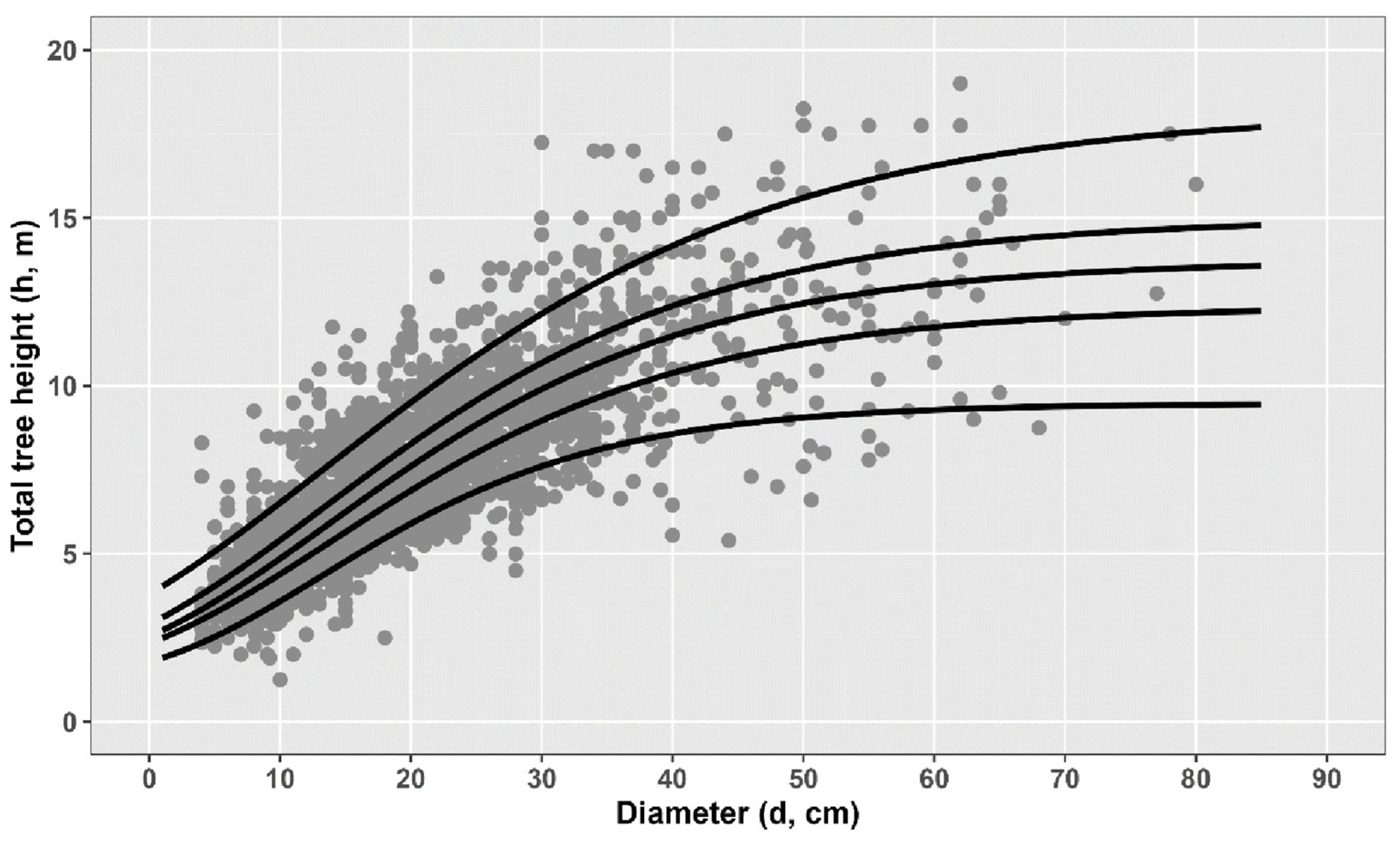
According to the QR approach utilized, compared to the FE model, all three QR models produced better MD and MAD values when for all calibration sizes (1 < m < 5). The results exhibited that the 3QR was consistently worse than the 5QR and 9QR models. The five-QR approach predicted tree height slightly better overall. As discussed by Bohora and Cao [90], this could be the case of over-fitting in which the extra curves based on 0.3 and 0.7 quantiles were ineffective and might cause a minor loss in terms of performance compared to the simpler QR system.

Zang et al. [28] applied a generalized h–d model at the fifty percent quantile without performing any calibration. In contrast, other studies have calibrated QR models using a single observation, such as a measured diameter at a specific age [90] or a measured stem diameter at a particular tree height [38]. As indicated by Xie et al. [41], determining the appropriate number of the pre-measured subsample trees also appears to be essential, directly affecting time and cost of the forest inventory. This study’s results showed that the base equation’s prediction ability was improved by using a subset of tree height values for each plot to calibrate the model. Earlier studies showed that an increase in sampling effort improves the ability of the models in terms of prediction [13,23,89]. The current research showed that as the number of trees used for calibration of different modeling approaches increased, the fit index values of the models used increased, while MAD and RMSE values decreased. Considering the results obtained, it was concluded that four randomly selected sample trees from each sample area would be sufficient for calibration, considering the balance between increased prediction accuracy and sampling cost. Teshome et al. [23] used 3 trees, Calama and Montero [7] used 4 trees for calibration, Temesgen et al. [89] suggested using between 1–15 trees for calibration, while Huang et al. [13] suggested using 6 or more trees for calibration. Ciceu et al. [19] and Xie et al. [41] stated that selecting six trees from each sample area would be sufficient to calibrate different modeling approaches. On the other hand, Temesgen et al. [26] stated that three trees from each sample area would be sufficient for calibration and that using more sample trees would not significantly affect prediction performance. Finally, Sharma and Parton [91] stated that for model calibration in general, considering the balance between the model’s estimation performance and the cost of data collection, the use of trees ranging from four to nine trees would be appropriate.

To inform future height–diameter (h–d) modeling studies across different tree species, a comparison of this study’s findings with previous research [9,12,13,14,15,16,17,18,19,26,27,28,29,53] shows that accurate and reliable tree height predictions can be achieved using ME models, even without incorporating additional stand-level variables such as H₀, D₀, number of trees (N), and G. This holds true across diverse climatic conditions and forest structures. As a result, the ME modeling technique has gained prominence in h–d modeling due to its ability to effectively capture variation in tree height–diameter relationships across different forest types, species compositions, and climate zones.

Because measuring tree height is often challenging and time-consuming, particularly in tropical forests and areas with dense broad-leaved canopies where treetops are obscured, h–d models serve as a practical alternative for estimating tree heights. According to this study, the ME model outperformed the QR model in prediction accuracy. Furthermore, the predictive performance of h–d models can be significantly enhanced by calibrating them with prior information. However, when considering sampling costs such as labor and time, measuring the heights of four or five trees per sample plot is sufficient to calibrate the model effectively for both the ME and QR techniques.

4.2. ML Modeling

Since ML offers key advantages over traditional modeling, as it avoids assumptions, eliminates the need for statistical testing, and does not require calibration strategies, we explored different ML approaches that are appropriate for the data’s size and biological variability.

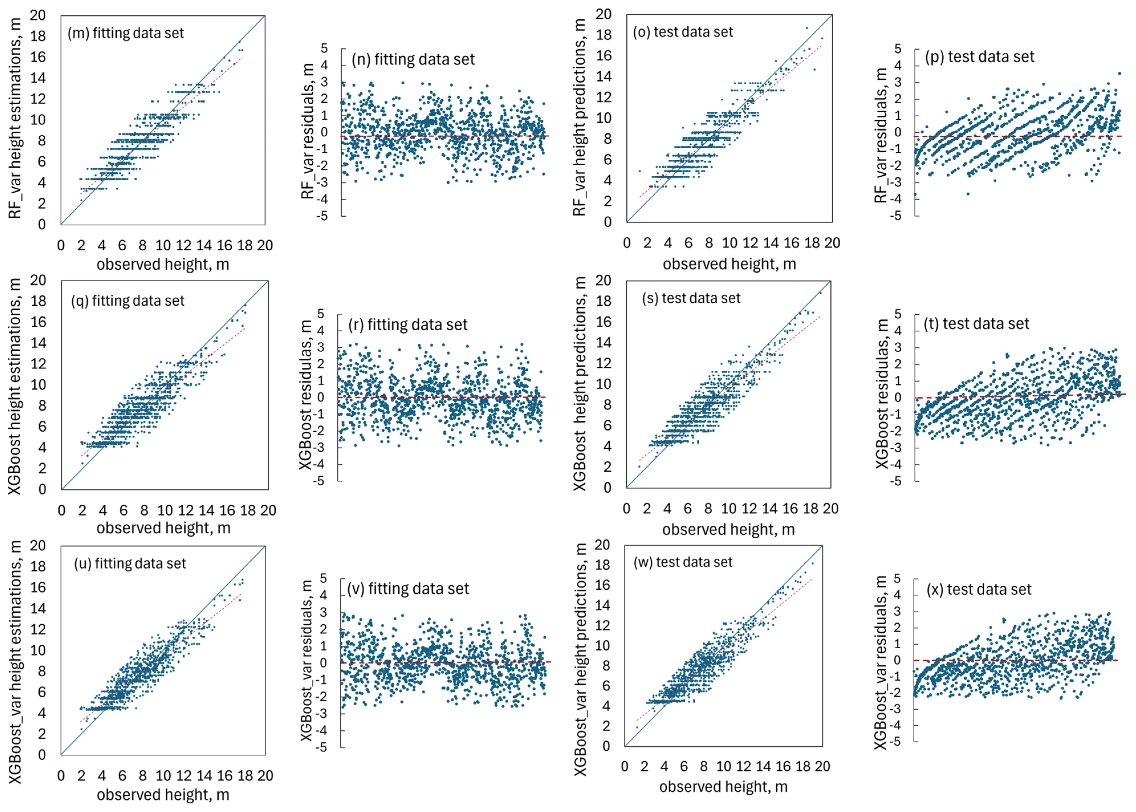
To ensure a fair and meaningful comparison between the ML models and the parametric models, two types of ML models were developed. The first type did not account for diameter variability and was designed to be directly comparable to the FE and QR models. The second type incorporated diameter variability among the k sample plots as input information, making it comparable to the ME, MCR, and MG models, which also utilize this variability. Following this approach, the results (Table 7) demonstrate that the ML models outperformed under both conditions. Specifically, ML models showed superior adaptability to the data regardless of whether or not diameter variability was included. Notably, even the ML models that excluded diameter variability outperformed the MCR and MG models that did include this information (Table 7). Furthermore, to ensure a fair comparison across all modeling approaches, predictive performance was assessed only under the condition that none of the models were calibrated (Table 8). It was further observed that the ML constructed models, even when using only diameter at breast height as input, outperformed the ME models, which incorporated additional information across all calibration scenarios (Table 7 and Table 9).

Our results were in line with most of the current research outcomes. Zhang et al. [92] highlighted the XGBoost algorithm’s superiority as compared to other ML algorithms along with its effectiveness in large-scale forest height estimation, while Fisher et al. [93], dealing with map timber harvest types and ages, suggested the use of XGBoost algorithm, which can effectively work with light detection and ranging (LiDAR) metrics and forest harvest data as model predictors. On the other hand, Fareed and Numata [94] evaluated different ML approaches and concluded that the RF algorithm produced the most accurate above ground biomass estimates for dense tropical canopy conditions, when tree height error correction is applied. Furthermore, recent studies have shown that finding accurate and reliable h–d relationships is challenging, requiring new and robust methodologies to be applied for this task [49,50,51,52,53,54,55]. On the other hand, parametric, semi-parametric, and ML models were tested [95] for h–d model construction and it was found that the semi-parametric generalized additive model can provide the most accurate results. For this reason, further research is required across a broader range of tree species and forest attributes for the general performance and behavior of different machine learning algorithms to be explored.

4.3. Comparative Effectiveness of Modeling Approaches Used

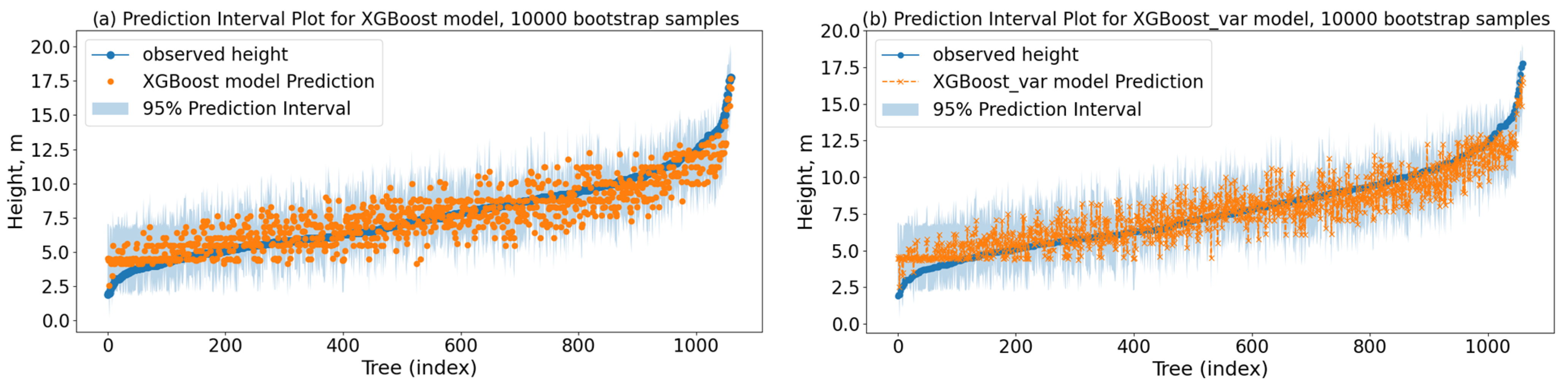
Based on the results obtained, the XGBoost modeling approach, without applying any calibration strategy, demonstrated the highest accuracy (Table 7 and Table 9) and reliability (Table 8) among the evaluated models. Specifically, the estimation RMSE values (Table 7) produced by the XGBoost model were reduced by 23.3%, 8.4%, and 7.28% compared to the FE, MCR, and MG models, respectively, and by 2.2% and 1.6% compared to the S_MLP and RF models, respectively. Similarly, the XGBoost_var model, which accounts for plot variability, achieved estimation RMSE reductions of 5.1%, 14.4%, 13.9%, and 14.7% compared to the ME, 3QR, 5QR, and 9QR models, respectively, and reductions of 3.8% and 2.6% compared to the S_MLP_var and RF_var models.

A consistent trend was observed in the prediction RMSE values (Table 8), where the XGBoost model again outperformed others, with reductions ranging from 26.5% to 1.1% relative to the FE, MCR, MG, S_MLP, and RF models.

Taking into account the results derived by the ML approaches, whether they take into account the variability among plots or not, they can work very well with moderate-sized datasets, as the available dataset showed their flexibility along with their ability to handle the inherent nonlinearities of the total tree height by producing adequate h–d models. However, drawbacks are hidden behind each ML modeling technique, which has to be taken into account in order to select the most appropriate for each different task. Although it is not required for ensemble methodologies, feature scaling is used in all approaches to apply a proper methodological approach to the problem. Furthermore, shallow MPL is not as robust to overfit as the two ensemble methodologies are, while the ensemble methodologies are of higher accuracy. Still, at the same time, they require more effort and computational time for their numerous hyperparameter tunings.

Taking into account the complexity of each modeling system investigated, the requirements that must be met either in terms of field or office work, and finally taking into account the accuracy and reliability of the estimates and predictions it produced, as well as the practical application of each modeling strategy, it seems that the XGBoost can be considered as a valuable alternative to parametric modeling and a reliable technique as compared to the rest of the ML modeling techniques explored for h–d model development.

5. Conclusions

Reliable h–d model construction is fundamental in forest management practice, since it can significantly help in forest productivity assessments, carbon accounting and sustainable harvest planning and can effectively support forest growth and yield modeling. Furthermore, the combination of accurate h–d models with Unmanned Aerial Vehicles and LiDAR can enable forest monitoring and mapping, reducing field inventory efforts.

Parametric and non-parametric h–d models were developed for Juniperus excelsa (Crimean juniper) using various advanced modeling techniques, including FE, ME, QR, S_MLP, RF, and XGBoost.

Multiple calibration strategies were applied to parametric models, with the ME approach consistently outperforming others across all calibration sample sizes. Notably, ME models achieved high predictive accuracy without requiring additional stand-level covariates. The fifth quantile (5QR) model yielded the most precise predictions among the QR approaches. Among the QR models tested, the 5QR model produced the highest accuracy. Finally, expanding sample size localization from four to five trees had only a negligible impact on the accuracy of estimations for Crimean juniper, supporting that beyond a certain threshold, adding more sample trees does not significantly enhance the predictive capability of the models.

Non-parametric ML models operate independently of calibration and distributional assumptions and demonstrate strong potential in modeling the complex, nonlinear relationship between tree height and breast height diameter. Among these, XGBoost exhibited superior predictive accuracy and reliability, outperforming S_MLP, RF, and all parametric alternatives. Specifically, it reduced RMSE values by 23.3%, 8.4%, and 7.28% compared to the FE, MCR, and MG models, respectively, and by 2.2% and 1.6% compared to the S_MLP and RF models.

Given the comparative advantages in handling moderate-sized, nonlinear datasets, which is a common scenario in forest modeling, XGBoost emerges as a robust and effective tool for h–d model development, which is fundamental in forest management practice. That is, the XGBoost approach can offer a reliable alternative to traditional parametric methods. This approach is thought to be able to significantly help in forest productivity assessments, carbon accounting, sustainable harvest planning, and effectively support forest growth and yield modeling. Furthermore, combining accurate h–d models with Unmanned Aerial Vehicles and LiDAR can significantly boost forest monitoring and mapping, reducing field inventory efforts.

References

1. GDF. Forest Resources; The General Directorate of Forests: Ankara, Türkiye, 2023; pp. 1–32. [Google Scholar]
2. GDF. Ecosystem-Based Multifunctional Forest Planning Guidelines (Code No: 299); The Turkish General Directorate of Forestry: Ankara, Turkey, 2017. (In Turkish) [Google Scholar]
3. Castaño-Santamaría, J.; Crecente-Campo, F.; Fernández-Martínez, J.L.; Barrio-Anta, M.; Obeso, J.R. Tree height prediction approaches for uneven-aged beech forests in northwestern Spain. For. Ecol. Manag. 2013, 307, 63–73. [Google Scholar] [CrossRef]
4. Curtis, R.O. Height-diameter and height-diameter-age equations for second-growth Douglas-fir. For. Sci. 1967, 13, 365–375. [Google Scholar] [CrossRef]
5. Parresol, B.R. Baldcypress height–diameter equations and their prediction confidence interval. Can. J. For. Res. 1992, 22, 1429–1434. [Google Scholar] [CrossRef]
6. Morrison, M.L.; Marcot, B.G.; Mannan, R.W. Wildlife Habitat Relationships: Concepts and Applications, 2nd ed.; University Wisconsin Press: Madison, WI, USA, 1992; 448p. [Google Scholar]
7. Calama, R.; Montero, G. Interregional nonlinear height diameter model with random coefficients for stone pine in Spain. Can. J. For. Res. 2004, 34, 150–163. [Google Scholar] [CrossRef]
8. Newton, P.F.; Amponsah, I.G. Comparative evaluation of five height–diameter models developed for black spruce and jack pine stand-types in terms of goodness-of-fit, lack-of-fit and predictive ability. For. Ecol. Manag. 2007, 247, 149–166. [Google Scholar] [CrossRef]
9. Crecente-Campo, F.; Tome, M.; Soares, P.; Dieguez-Aranda, U. A generalized nonlinear-mixed-effects height-diameter model for Eucalyptus globulus L. northwestern Spain. For. Ecol. Manag. 2010, 259, 943–952. [Google Scholar] [CrossRef]
10. Corral-Rivas, S.; Álvarez-González, J.G.; Crecente-Campo, F.; Corral-Rivas, J.J. Local and generalized height-diameter models with random parameters for mixed, uneven-aged forests in Northwestern Durango, Mexico. For. Ecosyst. 2014, 1, 6. [Google Scholar] [CrossRef]
11. Kearsley, E.; Moonen, P.C.; Hufkens, K.; Doetterl, S.; Lisingo, J.; Bosela, F.B.; Boeckx, P.; Beeckman, H.; Verbeeck, H. Model performance of tree height-diameter relationships in the central Congo Basin. Ann. For. Sci. 2017, 74, 7. [Google Scholar] [CrossRef]
12. Sharma, M.; Parton, J. Height–diameter equations for boreal tree species in Ontario using a mixed-effects modeling approach. For. Ecol. Manag. 2007, 249, 187–198. [Google Scholar] [CrossRef]
13. Huang, S.; Wiens, D.P.; Yang, Y.; Meng, S.X.; Vanderschaaf, C.L. Assessing the impacts of species composition, top height and density on individual tree height prediction of quaking aspen in boreal mixed woods. For. Ecol. Manag. 2009, 258, 1235–1247. [Google Scholar] [CrossRef]
14. Lhotka, J.M. Height-diameter relationships in Sweetgum (Liquidambar styraciflua)-dominated stands. South. J. Appl. For. 2012, 36, 98–106. [Google Scholar] [CrossRef]
15. Özçelik, R.; Diamantopoulou, M.J.; Crecente-Campo, F.; Eler, U. Estimating Crimean juniper tree height using nonlinear regression and artificial neural network models. For. Ecol. Manag. 2013, 306, 52–60. [Google Scholar] [CrossRef]
16. Gómez-García, E.; Diéguez-Aranda, U.; Castedo-Dorado, F.; Crecente-Campo, F.A. Comparison of Model Forms for the Development of Height-Diameter Relationships in Even-Aged Stands. For. Sci. 2014, 60, 560–568. [Google Scholar] [CrossRef]
17. Gómez-García, E.; Fonseca, T.F.; Crecente-Campo, F.; Almeida, L.R.; Dieguez-Aranda, U.; Huang, S.; Marques, C.P. Height-diameter models for maritime pine in Portugal: A comparison of basic, generalized and mixed-effects models. iForest-Biogeosciences For. 2015, 9, 72–78. [Google Scholar] [CrossRef]
18. Özçelik, R.; Cao, Q.V.; Trincado, G.; Göçer, N. Predicting tree height from tree diameter and dominant height using mixed-effects and quantile regression models for two species in Türkiye. For. Ecol. Manag. 2018, 419, 240–248. [Google Scholar] [CrossRef]
19. Ciceu, A.; Garcia-Duro, J.; Seceleanu, I.; Badea, O. A generalized nonlinear mixed-effects height–diameter model for Norway spruce in mixed-uneven aged stands. For. Ecol. Manag. 2020, 477, 118507. [Google Scholar] [CrossRef]
20. Bronisz, K.; Mehtätalo, L. Mixed-effects generalized height–diameter model for young silver birch stands on post-agricultural lands. For. Ecol. Manag. 2020, 460, 117901. [Google Scholar] [CrossRef]
21. Siipiletho, J.; Sarkkola, S.; Nuutinen, Y.; Mehtätalo, L. Predicting height-diameter relationship in uneven-aged stands in Finland. For. Ecol. Manag. 2023, 549, 121486. [Google Scholar] [CrossRef]
22. Raptis, D.I.; Papadopoulou, D.; Psarra, A.; Fallias, A.; Tsitsanis, A.; Kazana, V. Height-diameter models for King Borsi fir (Abies borisii regis Mattf.) and Scots pine (Pinus sylvestris L.) in Olympus and Pieria Mountains, Greece. J. Mt. Sci. 2024, 21, 1475–1490. [Google Scholar] [CrossRef]
23. Teshome, M.; Braz, E.M.; Torres, C.M.M.E.; Raptis, D.I.; de Mattos, P.P.; Temesgen, H.; Rubio-Camacho, E.A.; Sileshi, G.W. Mixed-Effects Height Prediction Model for Juniperus procera Trees from a Dry Afromontane Forest in Ethiopia. Forests 2024, 15, 443. [Google Scholar] [CrossRef]
24. Meng, S. Species-specific and generalized allometric biomass models for eight Fagaceae species in the understory of evergreen broadleaved forests in subtropical China. J. For. Res. 2024, 35, 69. [Google Scholar] [CrossRef]
25. Adame, P.; del Río, M.; Canellas, I. A mixed nonlinear height–diameter model for pyrenean oak (Quercus pyrenaica Willd.). For. Ecol. Manag. 2008, 256, 88–98. [Google Scholar] [CrossRef]
26. Temesgen, H.; Zhang, C.H.; Zhao, X.H. Modelling tree height–diameter relationships in multi-species and multi-layered forests: A large observational study from Northeast China. For. Ecol. Manag. 2014, 316, 78–89. [Google Scholar] [CrossRef]
27. Trincado, G.; VanderSchaaf, C.L.; Burkhart, H.E. Regional mixed-effects height–diameter models for loblolly pine (Pinus taeda L.) plantations. Eur. J. For. Res. 2007, 126, 253–262. [Google Scholar] [CrossRef]
28. Zang, H.; Lei, X.; Zeng, W. Height–diameter equations for larch plantations in northern and northeastern China: A comparison of the mixed-effects, quantile regression and generalized additive models. For. Int. J. For. Res. 2016, 89, 434–445. [Google Scholar] [CrossRef]
29. Han, Y.; Lei, Z.; Ciceu, A.; Zhou, Y.; Zhou, F.; Yu, D. Determining an accurate and cost effective individual height-diameter model for Mongolian pine on sandy land. Forests 2021, 12, 1144. [Google Scholar] [CrossRef]
30. Chenge, I.B. Height–diameter relationship of trees in Omo strict nature forest reserve, Nigeria. Trees For. People 2021, 3, 100051. [Google Scholar] [CrossRef]
31. Mehtätalo, L.; de-Miguel, S.; Gregoire, T.G. Modeling height-diameter curves for prediction. Can. J. For. Res. 2015, 45, 826–837. [Google Scholar] [CrossRef]
32. Pinheiro, J.C.; Bates, D.M. Linear Mixed-Effects Models: Basic Concepts and Examples. Mixed-Effects Models in S and S-Plus. In Mixed-Effects Models in S and S-PLUS. Statistics and Computing; Springer: New York, NY, USA, 2000; pp. 3–56. [Google Scholar] [CrossRef]
33. Sharma, M. Comparing Height-Diameter Relationships of Boreal Tree Species Grown in Plantations and Natural Stands. For. Sci. 2016, 62, 70–77. [Google Scholar] [CrossRef]
34. Koenker, R.; Bassett, G., Jr. Regression quantiles. Econom. J. Econom. Soc. 1978, 46, 33–50. [Google Scholar] [CrossRef]
35. Ducey, M.J.; Knapp, R.A. A stand density index for complex mixed species forests in the northeastern United States. For. Ecol. Manag. 2010, 260, 1613–1622. [Google Scholar] [CrossRef]
36. Zhang, L.; Bi, H.; Gove, J.H.; Heath, L.S. A comparison of alternative methods for estimating the self-thinning boundary line. Can. J. For. Res. 2005, 35, 1507–1514. [Google Scholar] [CrossRef]
37. Russell, M.B.; Weiskittel, A.R. Maximum and stand-level crown width equations for 15 tree species in Maine. North. J. Appl. For. 2011, 28, 84–91. [Google Scholar] [CrossRef]
38. Evans, A.M.; Gregoire, T.G. A geographically variable model of hemlock woolly adelgid spread. Biol. Invasions 2007, 9, 369–382. [Google Scholar] [CrossRef]
39. Cao, Q.V.; Wang, J. Evaluation of methods for calibrating a tree taper equation. For. Sci. 2015, 61, 213–219. [Google Scholar] [CrossRef]
40. Schmidt, M.; Kiviste, A.; von Gadow, K. A spatially explicit height–diameter model for Scots pine in Estonia. Eur. J. For. Res. 2011, 130, 303–315. [Google Scholar] [CrossRef]
41. Xie, L.; Widagdo, F.R.A.; Miao, Z.; Dong, L.; Li, F. Evaluation of the mixed-effects model and quantile regression approaches for predicting tree height in larch (Larix olgensis) plantations in northeastern China. Can. J. For. Res. 2022, 52, 309–319. [Google Scholar] [CrossRef]
42. Ciceu, A.; Chakraborty, D.; Ledermann, T. Examining the transferability of height-diameter model calibration strategies across studies. For. Int. J. For. Res. 2023, cpad063. [Google Scholar] [CrossRef]
43. Muggeo, V.M.R.; Sciandra, M.; Tomasello, A.; Calvo, S. Estimating growth charts via nonparametric quantile regression: A practical framework with application in ecology. Environ. Ecol. Stat. 2013, 20, 519–531. [Google Scholar] [CrossRef]
44. Liu, C.; Zhang, L.; Davis, C.J.; Solomon, D.S.; Brann, T.B.; Caldwell, L.E. Comparison of neural networks and statistical methods in classification of ecological habitats using FIA data. For. Sci. 2003, 49, 619–631. [Google Scholar] [CrossRef]
45. Diamantopoulou, M.J.; Milios, E.; Doganos, D.; Bistinas, I. Artificial neural network modeling for reforestation design through the dominant trees bole-volume estimation. Nat. Resour. Model. 2009, 22, 511–543. [Google Scholar] [CrossRef]
46. Soares, F.A.A.; Flores, E.L.; Cabacinha, C.D.; Carrijo, G.A.; Veiga, A.C.P. Recursive diameter prediction for calculating merchantable volume of eucalyptus clones using Multilayer Perceptron. Neural Comput. Appl. 2013, 22, 1407–1418. [Google Scholar] [CrossRef]
47. Cosenza, D.N.; Soares, A.A.V.; De Alcantara, A.E.M.; Da Silva, A.A.L.; Rode, R.; Soares, V.P.; Leite, H.G. Site classification for eucalypt stands using artificial neural network based on environmental and management features. Cerne 2017, 23, 310–320. [Google Scholar] [CrossRef]
48. Ercanli, I.; Günlü, A.; Şenyurt, M.; Keles, S. Artificial neural network models predicting the leaf area index: A case study in pure even-aged Crimean pine forests from Turkey. For. Ecosyst. 2018, 5, 29. [Google Scholar] [CrossRef]
49. Sun, Y.; Ao, Z.; Jia, W.; Chen, Y.; Xu, K. A geographically weighted deep neural network model for research on the spatial distribution of the down dead wood volume in Liangshui National Nature Reserve (China). iFor.-Biogeosci. For. 2021, 14, 353–361. [Google Scholar] [CrossRef]
50. Li, Y.; Jiang, L. Application of ANN algorithm in tree height modeling. Appl. Mech. Mater. 2010, 20–23, 756–761. [Google Scholar] [CrossRef]
51. Thanh, T.N.; Tien, T.D.; Shen, H.L. Height-diameter relationship for Pinus koraiensis in Mengjiagang Forest Farm of Northeast China using nonlinear regressions and artificial neural network models. J. For. Sci. 2019, 65, 134–143. [Google Scholar] [CrossRef]
52. Karatepe, Y.; Diamantopoulou, M.J.; Özçelik, R.; Sürücü, Z. Total tree height predictions via parametric and artificial neural network modeling approaches. iFor.-Biogeosci. For. 2022, 15, 95–105. [Google Scholar] [CrossRef]
53. Ogana, F.N.; Ercanli, I. Modelling height-diameter relationships in complex tropical rain forest ecosystems using deep learning algorithm. J. For. Res. 2022, 33, 883–898. [Google Scholar] [CrossRef]
54. Ou, Y.; Quiñónez-Barraza, G. Modeling Height–Diameter Relationship Using Artificial Neural Networks for Durango Pine (Pinus durangensis Martínez) Species in Mexico. Forests 2023, 14, 1544. [Google Scholar] [CrossRef]
55. Şahin, A.; Aylak Ozdemir, G.; Oral, O.; Aylak, B.L.; Ince, M.; Ozdemir, E. Estimation of tree height with machine learning techniques in coppice-originated pure sessile oak (Quercus petraea (Matt.) Liebl.) stands. Scand. J. For. Res. 2023, 38, 87–96. [Google Scholar] [CrossRef]
56. Xuan, J.; Li, X.; Du, H.; Zhou, G.; Mao, F.; Wang, J.; Zhang, B.; Gong, Y.; Zhu, D.; Zhou, L.; et al. Intelligent Estimating the Tree Height in Urban Forests Based on Deep Learning Combined with a Smartphone and a Comparison with UAV-LiDAR. Remote Sens. 2023, 15, 97. [Google Scholar] [CrossRef]
57. Friedman, F.H. Greedy function approximation: A gradient boosting machine. Ann. Statist. 2001, 29, 1189–1232. [Google Scholar] [CrossRef]
58. Chen, T.; Guestrin, C. XGBoost: A Scalable Tree Boosting System. In Proceedings of the 22nd ACM SIGKDD: International Conference on Knowledge Discovery and Data Mining, KDD, San Francisco, CA, USA, 13–17 August 2016; pp. 785–794. [Google Scholar] [CrossRef]
59. Goodfellow, I.; Bengio, Y.; Courville, A. Deep Learning. Adaptive Computation and Machine Learning Series; MIT Press: Cambridge, MA, USA, 2016; 785p. [Google Scholar]
60. Alshboul, O.; Shehadeh, A.; Almasabha, G.; Almuflih, A.S. Extreme Gradient Boosting-Based Machine Learning Approach for Green Building Cost Prediction. Sustainability 2022, 14, 6651. [Google Scholar] [CrossRef]
61. Refaeilzadeh, P.; Tang, L.; Liu, H. Cross-Validation. In Encyclopedia of Database Systems; Lıu, L., Özsu, M.T., Eds.; Springer: Boston, MA, USA, 2009; pp. 532–538. [Google Scholar] [CrossRef]
62. Marcot, B.G.; Hanea, A.M. What is an optimal value of k in k-fold cross-validation in discrete Bayesian network analysis? Comput. Stat. 2020, 52, 667–692. [Google Scholar] [CrossRef]
63. Richards, F.J. A flexible growth curve for empirical use. J. Exp. Bot. 1959, 10, 290–300. [Google Scholar] [CrossRef]
64. Fang, Z.; Bailey, R.L. Height–diameter models for tropical forests on Hainan Island in southern China. For. Ecol. Manag. 1998, 110, 315–327. [Google Scholar] [CrossRef]
65. Huang, S.; Titus, S.J.; Wiens, D.P. Comparison of nonlinear height–diameter functions for major Alberta tree species. Can. J. For. Res. 1992, 22, 1297–1304. [Google Scholar] [CrossRef]
66. Raptis, D.I.; Kazana, V.; Kazaklis, A.; Stamatiou, C. Mixed-effects height-diameter models for black pine (Pinus nigra Arn.) forest management. Trees 2021, 35, 1167–1183. [Google Scholar] [CrossRef]
67. Institute Inc. SAS/SHARE® 9.4: User’s Guide, 2nd ed.; SAS Institute Inc.: Cary, NC, USA, 2016. [Google Scholar]
68. Meng, S.X.; Huang, S. Improved calibration of nonlinear mixed-effects models demonstrated on a height growth function. For. Sci. 2009, 55, 238–248. [Google Scholar] [CrossRef]
69. Maier, H.R.; Dandy, G.C. Neural networks for the prediction and forecasting of water resources variables: A review of modeling issues and applications. Environ. Model. Softw. 2000, 15, 101–124. [Google Scholar] [CrossRef]
70. Pedregosa, F.; Varoquaux, G.; Gramfort, A.; Michel, V.; Thirion, B.; Grisel, O.; Blondel, M.; Prettenhofer, P.; Weiss, R.; Dubourg, V.; et al. Scikit-learn: Machine learning in Python. J. Mach. Learn. Res. 2011, 12, 2825–2830. [Google Scholar] [CrossRef]
71. Python Software Foundation. Python Language Reference, version 3.13.2; Python Software Foundation: Beaverton, OR, USA, 2023; Available online: http://www.python.org (accessed on 5 May 2025).
72. McCulloch, W.S.; Pitts, W.H. A logical calculus of the ideas immanent in nervous activity. Bull. Math. Biophys. 1943, 5, 115–133. [Google Scholar] [CrossRef]
73. Rosenblatt, F. The perceptron: A probabilistic model for information storage and organization in the brain. Psychol. Rev. 1958, 65, 386–408. [Google Scholar] [CrossRef] [PubMed]
74. Werbos, P.J. Beyond Regression: New Tools for Prediction and Analysis in the Behavioral Sciences. Ph.D. Thesis, Committee on Applied Mathematics, Harvard University, Cambridge, MA, USA, 1974. Available online: https://perceptrondemo.com/assets/PJW_thesis_Beyond_Regression_1974-4b63aa5f.pdf (accessed on 2 April 2025).
75. Werbos, P.J. Back propagation through time: What it does and how to do it. In Proceedings of the IEEE ’90: International Conference, Santa Clara, CA, USA, 22–24 October 1990; IEEE: New York, NY, USA, 1990; Volume 78, pp. 1550–1560. [Google Scholar] [CrossRef]
76. Rumelhart, D.; Hinton, G.; Williams, R. Learning representations by back-propagating errors. Nature 1986, 323, 533–536. [Google Scholar] [CrossRef]
77. Aggarwal, C. Machine Learning with Shallow Neural Networks. In Neural Networks and Deep Learning; Springer Nature: Berlin/Heidelberg, Germany; Switzerland AG: Zuerich, Switzerland, 2023; pp. 73–117. [Google Scholar] [CrossRef]
78. Sharma, S.; Sharma, S.; Athaiya, A. Activation functions in neural networks. Int. J. Eng. Appl. Sci. Technol. 2020, 4, 310–316. [Google Scholar] [CrossRef]
79. Tomar, A.; Laxkar, P. Differences of Tanh, sigmoid and ReLu Activation Function in Neural network. Int. J. Sci. Prog. Res. 2022, 80, 18–21. Available online: https://www.ijspr.com/citations/v80n6/IJSPR_8006_31035.pdf (accessed on 20 May 2025).
80. Kingma, D.P.; Ba, J. Adam: A Method for Stochastic Optimization. In Proceedings of the 3rd International Conference for Learning Representations, San Diego, CA, USA, 7–9 May 2015. [Google Scholar] [CrossRef]
81. Zhang, Z. Improved Adam Optimizer for Deep Neural Networks. In Proceedings of the IEEE/ACM 26th International Symposium on Quality of Service (IWQoS), Banff, AB, Canada, 4–6 June 2018; IEEE: New York, NY, USA, 2018; pp. 1–2. [Google Scholar] [CrossRef]
82. Breiman, L. Random Forests. Mach. Learn. 2001, 45, 5–32. [Google Scholar] [CrossRef]
83. Breskvar, M.; Kocev, D.; Džeroski, S. Ensembles for multi-target regression with random output selections. Mach. Learn. 2018, 107, 1673–1709. [Google Scholar] [CrossRef]
84. Shahhosseini, M.; Hu, G.; Pham, H. Optimizing ensemble weights and hyperparameters of machine learning models for regression problems. Mach. Learn. Appl. 2022, 7, 100251. [Google Scholar] [CrossRef]
85. Breiman, L. Bagging predictors. Mach. Learn. 1996, 26, 123–140. [Google Scholar] [CrossRef]
86. James, G.; Witten, D.; Hastie, T.; Tibshirani, R. An Introduction to Statistical Learning with Applications in R, 2nd ed.; Springer: New York, NY, USA, 2021; 607p. [Google Scholar] [CrossRef]
87. Chattopadhyay, G.; Sinha, B.K. Coverage probability and exact inference. J. Stat. Theory Pract. 2018, 12, 93–99. [Google Scholar] [CrossRef]
88. Castedo-Dorado, F.C.; Diéguez-Aranda, U.; Anta, M.B.; Rodríguez, M.S.; von Gadow, K. A generalized height–diameter model including random components for radiata pine plantations in northwestern Spain. For. Ecol. Manag. 2006, 229, 202–213. [Google Scholar] [CrossRef]
89. Temesgen, H.; Monleon, V.J.; Hann, D.W. Analysis and comparison of nonlinear tree height prediction strategies for Douglas-fir forests. Can. J. For. Res. 2008, 38, 553–565. [Google Scholar] [CrossRef]
90. Bohora, S.B.; Cao, Q.V. Prediction of tree diameter growth using quantile regression and mixed-effects models. For. Ecol. Manag. 2014, 319, 62–66. [Google Scholar] [CrossRef]
91. Sharma, M.; Parton, J. Modeling stand density effects on taper for jack pine and black spruce plantations using dimensional analysis. For. Sci. 2009, 55, 268–282. [Google Scholar] [CrossRef]
92. Zhang, N.; Chen, M.; Yang, F.; Yang, C.; Yang, P.; Gao, Y.; Shang, Y.; Peng, D. Forest Height Mapping Using Feature Selection and Machine Learning by Integrating Multi-Source Satellite Data in Baoding City, North China. Remote Sens. 2022, 14, 4434. [Google Scholar] [CrossRef]
93. Fisher, G.B.; Elmore, A.J.; Fitzpatrick, M.C.; McNeil, D.J.; Atkins, J.W.; Larkin, J.L. Mapping recent timber harvest activity in a temperate forest using single date airborne LiDAR surveys and machine learning: Lessons for conservation planning. GIScience Remote Sens. 2024, 61, 2379198. [Google Scholar] [CrossRef]
94. Fareed, N.; Numata, I. Evaluating the impact of field-measured tree height errors correction on aboveground biomass modeling using airborne laser scanning and GEDI datasets in Brazilian Amazonia. Trees For. People 2025, 19, 100751. [Google Scholar] [CrossRef]
95. Jha, S.; Yang, S.-I.; Brandeis, T.J.; Kuegler, O.; Marcano-Vega, H. Evaluation of regression methods and competition indices in characterizing height-diameter relationships for temperate and pantropical tree species. Front. For. Glob. Change 2023, 6, 1282297. [Google Scholar] [CrossRef]
Figure 1. Distribution of the natural juniper stands.
Forests 16 00972 g001
Figure 2. Plot of tree height (h) against the diameter (d) for fitting and test datasets.
Forests 16 00972 g002
Figure 3. Graphs of observed tree heights (gray dots) and curves generated by the QR based on five quantiles (black lines) for the test data.
Forests 16 00972 g003
Figure 4. 45-degree line and residual plots for the fitting dataset (a,b,e,f,i,j,m,n,q,r,u,v) and for the test dataset (c,d,g,h,k,l,o,p,s,t,w,x) for all ML constructed models.
Forests 16 00972 g004aForests 16 00972 g004b
Figure 5. 95% prediction intervals plot for the (a) XGBoost and (b) XGBoost_var constructed models, for the fitting dataset.
Forests 16 00972 g005