Article

Noninvasive Sonic Tomography for the Detection of Internal Defects in Relict Woodlands of Polylepis in Peru

by
Yakov Quinteros-Gómez
1,*,
Abel Salinas-Inga
1,2,
Jehoshua Macedo-Bedoya
1,2,*,
Enzo Peralta-Alcantara
1,
Marcel La Rosa-Sánchez
1,2,*,
Fernando Camones Gonzales
3,
Alexandra Yamunaque
1,4,
Franco Angeles-Alvarez
1,
Doris Gómez-Ticerán
2 and
Olga Lidia Solano Dávila
3
1
Laboratorio de Ecología Tropical y Análisis de Datos, Facultad de Ciencias Biológicas, Universidad Nacional Mayor de San Marcos (UNMSM), Lima 15081, Peru
2
Grupo de Investigación MOCA, Facultad de Ciencias Matemáticas, Universidad Nacional Mayor de San Marcos (UNMSM), Lima 15081, Peru
3
Departamento Académico de Estadística, Universidad Nacional Mayor de San Marcos (UNMSM), Lima 15081, Peru
4
Instituto de Ciencias Ómicas y Biotecnología Aplicada, Pontificia Universidad Católica del Perú, Lima 15088, Peru
*
Authors to whom correspondence should be addressed.
Forests 2025, 16(6), 957; https://doi.org/10.3390/f16060957
Submission received: 31 October 2024 / Revised: 14 May 2025 / Accepted: 26 May 2025 / Published: 5 June 2025
(This article belongs to the Section Forest Health)

Abstract

Polylepis woodlands, endemic to the Andean Mountains, are critical for biodiversity and ecosystem services but face threats from anthropogenic disturbances and climate change. This study employed sonic tomography (ST) to assess the structural integrity of three relict Polylepis stands on the western slopes of the Peruvian Andes. A total of 192 tomograms from 48 trees across three sites revealed substantial variation in internal decay (2.5–70%), with mean decay levels of 11.6% (Z1), 16.6% (Z2), and 10.5% (Z3). Although the initial generalized linear mixed models (GLMMs) suggested tree diameters at breast height (DBH) as a potential predictor of decay, subsequent non-parametric Spearman’s correlation analysis found no significant relationship between DBH and decay (r < 0.001, p > 0.05) or between altitude and decay (r = 0.187, p = 0.204). No significant differences were detected among species or zones. The study demonstrates the efficacy of ST for noninvasive health assessment in high-altitude ecosystems and underscores the need for long-term monitoring to guide conservation strategies.

1. Introduction

The Andes Mountains exert a profound influence on species connectivity, distribution, and spatiotemporal dynamics [1], functioning as a major biogeographical barrier [2,3] of significant ecological importance [4,5] that promotes speciation processes and high levels of endemism [6].
The Peruvian Western Slope (PWS), stretching from the southern border with Chile to the northern border with Ecuador, comprises a narrow region between the coastal strip and the summit line of the Western Andes [7]. This area harbors diverse ecosystems along an altitudinal gradient, from sea level to mountain ranges, including lomas formations, hills, xerophytic riparian forests, montane dry forests, shrublands, Andean grasslands, and wetlands [8]. Relict patches of Polylepis woodlands—locally known as queñua woodlands [9]—persist in the altitudinal belt between headwaters and periglacial zones [10,11].
The genus Polylepis, endemic to South America, comprises woody species with arboreal or shrubby habits, characterized by their multi-stemmed growth form and a maximum height of 20 m [12,13,14]. These trees exhibit remarkable longevity, with documented specimens exceeding 100 years and some individuals estimated to reach 1000 years [15,16,17].
Polylepis woodlands occur between 900 and 5000 m a.s.l. on mountain slopes and rocky ravines throughout the Andean Cordillera [13,18], with a distribution extending from the Venezuelan Andes to Northern Chile and Western Argentina [19,20]. Peru hosts the highest diversity and endemism of the genus [13,20], with populations documented in 19 of the country’s 24 departments and the highest concentrations in the central and southern highlands, particularly in Cuzco and Ayacucho [21,22].
Ecologically, Polylepis woodlands play a fundamental role in Andean ecosystems, with their distribution closely tied to watersheds [23], which provide the moisture conditions necessary for their establishment and persistence [24]. These woodlands facilitate hydrological regulation, maintaining continuous water flow in streams and rivers while contributing to slope stabilization and erosion control [25]. They also drive soil formation [26,27], thriving in rocky areas, and enhance substrate quality through nitrogen retention and nutrient cycling [28,29,30]. Additionally, Polylepis woodlands deliver critical ecosystem services, including carbon sequestration [31] and hydrological regulation [32,33], while providing habitats for endemic and threatened flora and fauna [34,35].
Despite the ecological significance of these woodlands [36], the health status (internal structure) of their populations remains poorly understood. These ecosystems have experienced significant degradation from anthropogenic activities, leading to substantial reductions in their extent and ecological integrity [13,37]. The primary threats to Polylepis woodlands include burning for agricultural expansion [38], livestock grazing [39], road infrastructure development [40], and firewood extraction by local communities [41,42,43].
Forest stand assessment protocols enable the evaluation of tree health and early detection of structural defects [44]. Approaches include multispectral remote sensing [45], satellite imagery analysis [46], and, increasingly, unmanned aerial vehicle (UAV) technology integrated with deep learning models for rapid, large-scale evaluations [47,48]. These aerial methods are complemented by field-based assessments [49] or invasive techniques such as wood drilling [50,51] and visual inspections of roots, trunks, and stems [52,53]. Recent advances in UAV-based methods using convolutional neural networks and other deep learning architectures have demonstrated high efficiency in detecting, locating, and quantifying structural defects and diseases across expansive forests [47,48].
Monitoring the internal tree structure is critical for detecting pathogens, fungal infections, and decay [54,55]. Internal cavities and decay zones significantly compromise the tree integrity, necessitating non-destructive assessment methods [56]. While hybrid deep learning approaches combined with UAV imagery excel at external defect detection [47], sonic tomography (ST) has emerged as a reliable, non-invasive tool for quantifying and visualizing internal decay in trunks, palm stems, and branches [57,58,59,60]. ST serves as a diagnostic tool for mapping decay, assessing tree failure risk in public areas [61,62], and guiding management planning [63,64]. It also supports evidence-based silvicultural decisions [65,66,67], complementing large-scale remote sensing for forest health monitoring [48].
To date, no studies have employed ST to evaluate the structural integrity of vulnerable natural populations such as Polylepis woodlands, leaving a critical knowledge gap for these ecologically vital Andean forests. This study addresses this gap by demonstrating the efficacy of acoustic tomography as a non-destructive health assessment tool for Andean forests, where species face varying threat levels according to the Peruvian Red Book of Endemic Plants [68]. Focusing on Polylepis woodlands under anthropogenic pressure, we provide baseline data on internal decay patterns in these climate-vulnerable ecosystems [69]. Understanding their structural health is urgent, as these forests face escalating conservation challenges, including habitat fragmentation, climate change impacts, and human disturbance [70,71]. The aim of this study was to assess the internal structural integrity of trees across three Polylepis woodland patches subjected to differing anthropogenic pressures, establishing ST as a viable conservation tool for monitoring threatened Andean ecosystems.

2. Materials and Methods
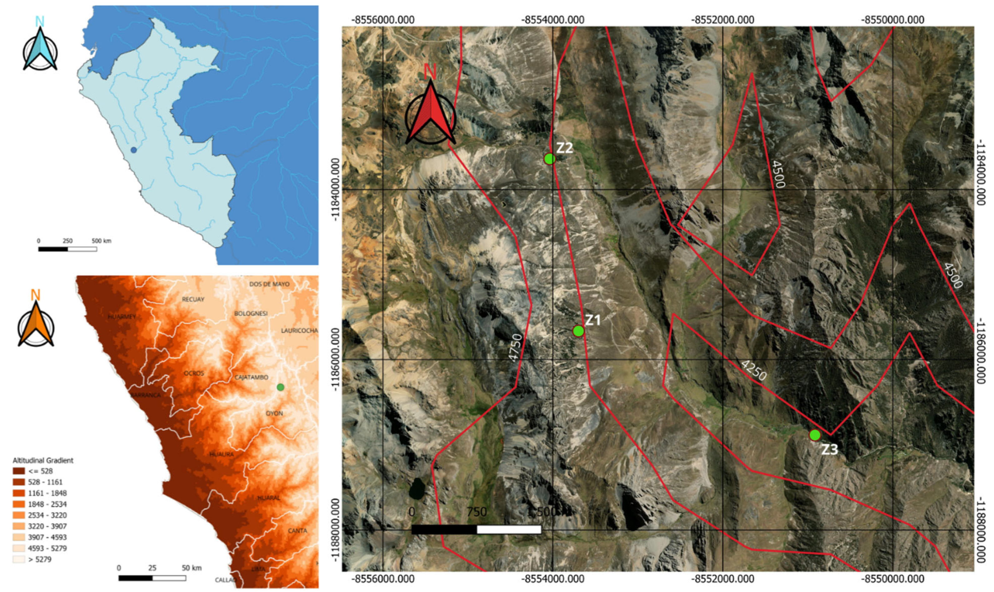
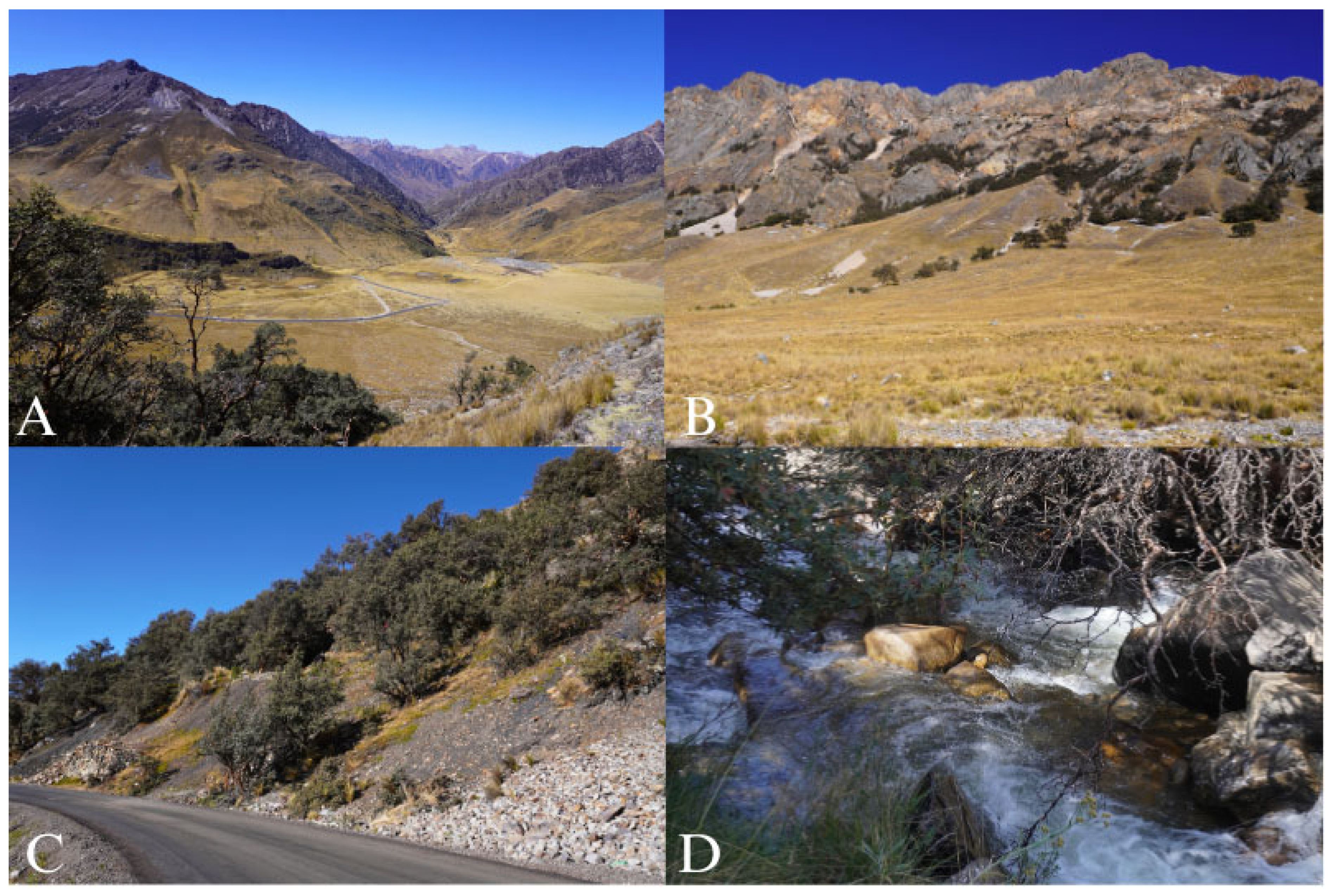
2.1. Study Sites

The study was conducted during the dry season (June–July 2024) in three relict woodlands of Queñua (Polylepis spp.) situated in the Huaura Watershed, Oyón Province, Lima Department, Peru. The study sites are distributed along western slopes of the Andes, adjacent to the Raura mountain range, at elevations ranging from 4000 to 4500 m a.s.l. (Figure 1). The sites experience variable climatic conditions [72], with mean temperatures ranging from 5.7 °C (minimum) to 16.8 °C (maximum) and a mean monthly precipitation of 2.45 mm [73].
Three relict Polylepis woodlands were selected for study (Figure 2). The first study site (Z1), located at 4350–4400 m a.s.l., is adjacent to the Oyón–Cajatambo Highway near Cashaucro in a landscape dominated by herbaceous vegetation with scattered shrubs. Above 4000 m elevation, there is a distinct edaphic transition from compacted soil with grassland cover to terrain increasingly dominated by rocky outcrops and loose stones. The second study site (Z2), situated at 4500 m a.s.l. along the Cajatambo–Raura Mine road, is surrounded by grassland dominated by Calamagrostis sp. and Stipa sp. Road construction has fragmented this woodland into three patches, resulting in selective tree removal. The third study site (Z3), occurring at 4000–4050 m a.s.l., is bisected by the Ushpa River and the main road, creating upper and lower woodland segments. Recent evidence of anthropogenic disturbance includes the extraction of Polylepis trunks, as confirmed by the presence of several large, felled specimens.
Three study sites (blocks) were considered for sampling. In each site, four plots (10 × 10 m) were established, and within each plot, four trees (DBH > 10 cm) were selected for measurement. For each tree, sensors were placed at four designated height levels on the trunk. This sampling design resulted in 64 observations per block and 192 observations overall. Tree selection followed four criteria: (i) accessibility to each tree, (ii) ensuring researcher safety by minimizing accident risks, (iii) preliminary visual assessment of the tree trunk to detect signs of external structural damage, and (iv) a minimum DBH > 10 cm.

2.2. Sonic Tomography

Prior to installation, all sensors were disinfected using a 70% alcohol solution followed by application of a broad-spectrum insecticide. Ten sensors and five transmitter boxes (connected to a laptop for data acquisition) were positioned at equidistant intervals around the circumference of each selected tree [65]. Each tree with DBH > 10 cm was assessed at four standardized height levels (10 cm, 30 cm, 50 cm, and 70 cm aboveground) (Figure 3A,B), enabling cross-sectional analysis by layer and subsequent generation of 3D tomograms [74].
Tomograms were generated by lightly tapping each sensor with a specialized hammer (Figure 3C), producing acoustic waves that propagated transversely through the trunk. Wave velocity was recorded by the sensors [75,76], with structural anomalies (cavities or decay) detected as perturbations in the wave trajectory and transmission speed. This methodology allowed precise quantification of the internal damage extent as a percentage of the trunk cross-sectional area [74,75].
Decay percentages for each height level were calculated using Arborsonic 3D v5.3.162 software (Figure 3D), yielding the average structural damage per tree. Damage severity was classified into three risk categories following Helmanto et al. [77]: high (>60% decay), moderate (30–60% decay), and low (<30% decay). Layer-specific damage averages were computed for each plot. Geographic coordinates were recorded using a Garmin GPSMAP® 67i unit (Garmin Ltd., Olathe, KS, USA). Comprehensive photographic documentation of the sampled trees was conducted, and botanical specimens were collected for taxonomic verification through comparison with herbarium vouchers and specialized literature [43,78,79]. The nomenclature followed W3-Tropics (www.tropicos.org, accessed on 1 August 2024), while the conservation status was assessed using IUCN Red List Criteria and Peruvian threatened species classifications (Decreto Supremo No. 043-2006-AG).

2.3. Data Analysis

The analytical approach began with exploratory data visualization to examine the relationships between independent variables (species, zones, plots, DBH, and altitude) and the dependent variable (average damage) across the four measurement layers. Box plot visualizations facilitated a preliminary assessment of how these factors influenced the damage patterns, providing initial insights into zonal and plot-level variations in tree health. For more robust statistical evaluation, we implemented non-parametric tests, including the Mann–Whitney U test for pairwise comparisons and the Kruskal–Wallis test for multi-group analyses. Complementary scatter plots elucidated potential associations between DBH, altitude, and average damage while also examining the interactions between spatial variables (zone and plot) and tree morphological characteristics.
Prior to formal hypothesis testing, we conducted normality diagnostics on all quantitative variables to verify the appropriateness of the non-parametric methods. This assessment confirmed the need for the Spearman’s rank correlation coefficient to evaluate bivariate relationships. Subsequently, we constructed a linear mixed effects model to assess the combined influence of the predictor variables. Diagnostic plots revealed violations of homoscedasticity and normality assumptions in the model residuals, prompting the application of a Box–Cox transformation to the response variable (average damage) to meet the parametric requirements while preserving the interpretability of the results.
All statistical computations and visualizations were performed in RStudio (version 4.3.0) using specialized mixed-modeling packages. The glmmTMB package [80] provided flexible tools for generalized linear mixed model specification, while lmer [81] facilitated traditional linear mixed effects model fitting. This dual-package approach ensured rigorous evaluation of both transformed and untransformed variable relationships while accounting for the hierarchical structure of our sampling design.

3. Results

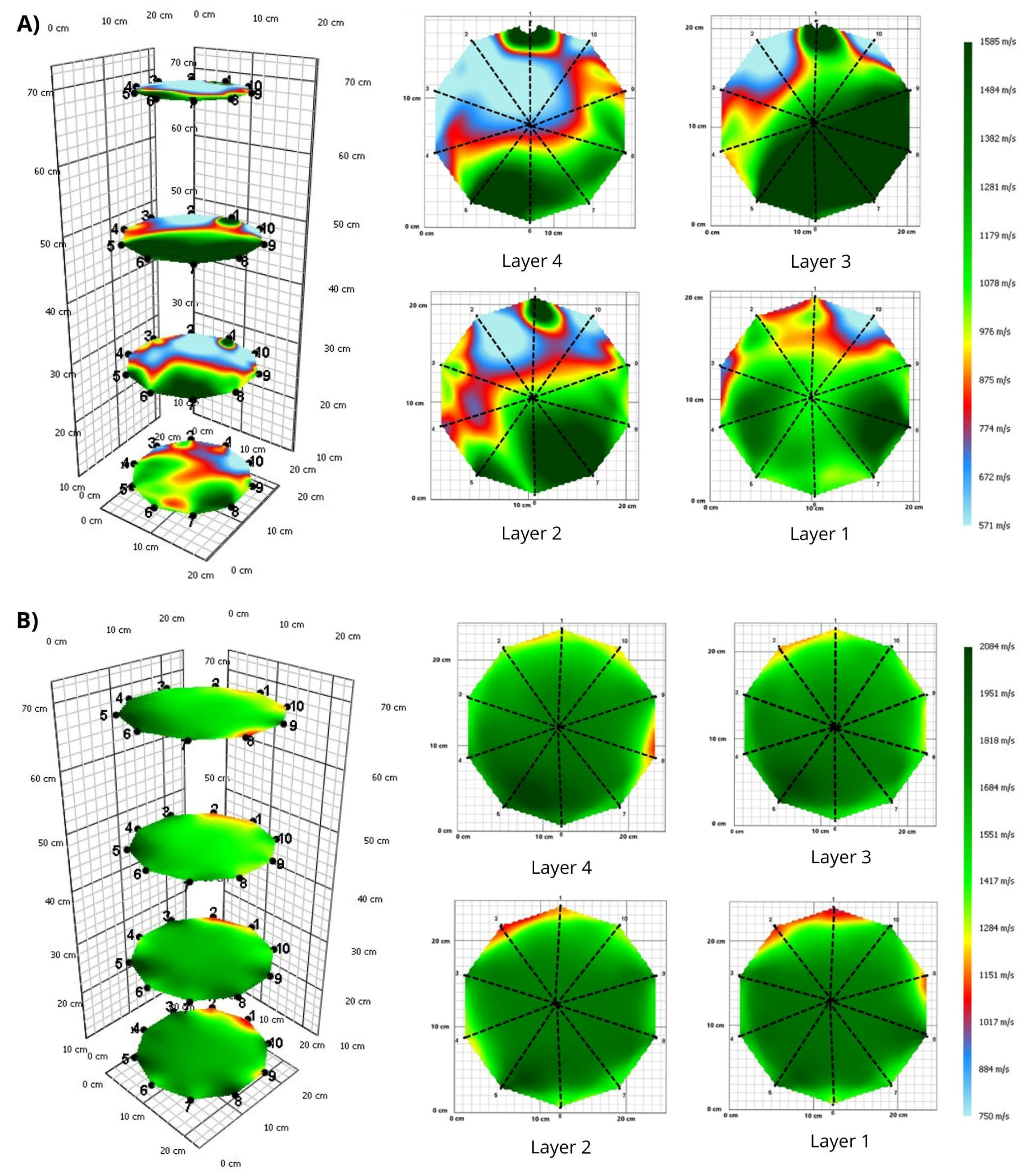
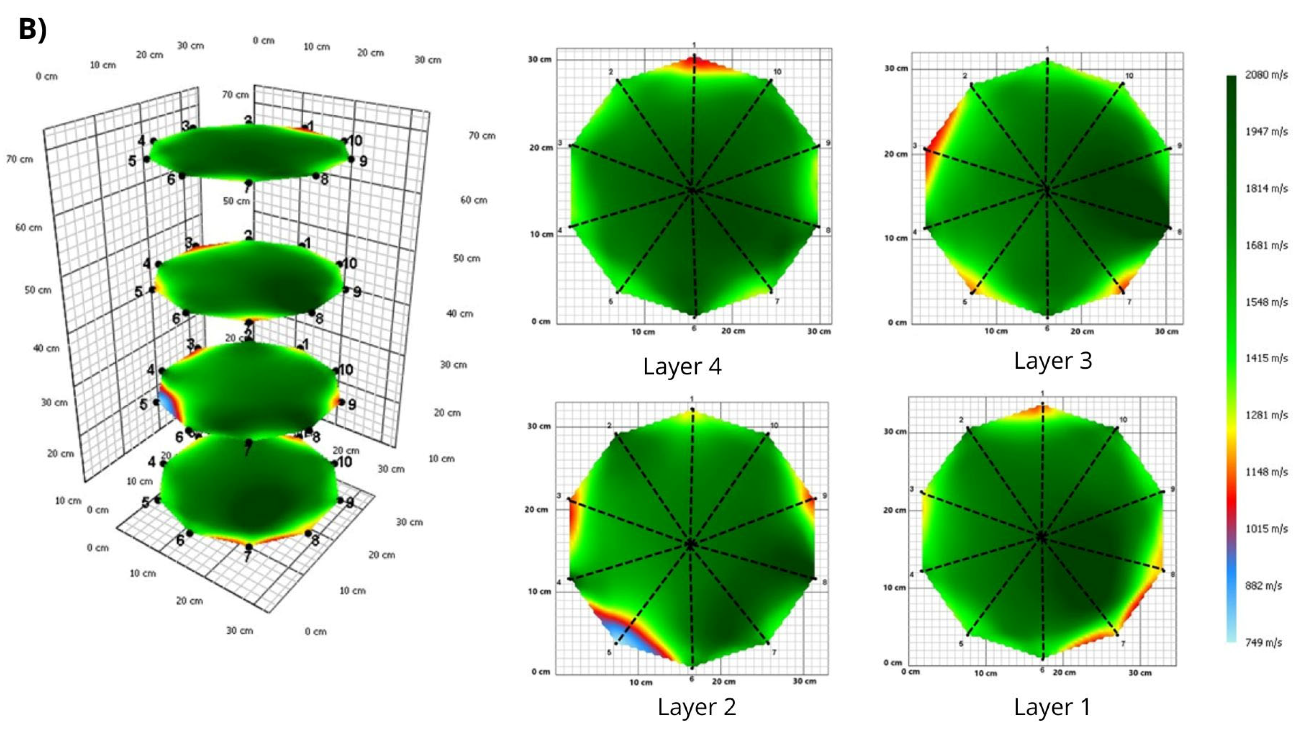
3.1. Tomograms and Level of Wood Decay

The sonic tomography analysis generated 192 tomograms across three study sites, revealing considerable variation in internal decay among the 48 assessed trees. The decay percentages ranged from minimally affected individuals (2.5–7%) to severely compromised specimens (maximum 70% decay) (Table 1).
Site Z1 exhibited a mean decay of 11.6%, with the most affected tree showing a distinct vertical decay gradient: 19% (basal layer), 44% (second layer), 23% (third layer), and 58% (uppermost layer). This pattern was primarily detected by sensors 2, 3, 4, and 10 (Figure 4A). In contrast, the least affected specimen maintained consistently low decay (1–4%) across all stem layers (Figure 4B). Site Z2 demonstrated the highest mean decay (16.6%) among all sites. The most compromised tree exhibited extensive damage (60–79%), concentrated in areas monitored by sensors 3, 7, and 8 (Figure 5A), while the healthiest specimen showed only minor decay (2–5%) (Figure 5B). Site Z3 displayed the lowest mean decay (10.5%), with the damage predominantly localized in the middle stem sections. The most affected tree showed peak decay in layer 2 (48%), followed by layers 3 (41%) and 4 (37%), consistently detected by sensors 1, 2, and 3 (Figure 6A). The least damaged specimen exhibited minimal decay (0–7%) with small, localized affected areas (Figure 6B).

3.2. Data Analysis Results

The box plot analysis for both Polylepis species revealed similar damage distributions, with median values ranging between 10% and 15% decay. However, outliers were present in both species, including one particularly extreme case in Polylepis weberbaueri Pilg, where the damage approached 70% (Figure 7a). Zone-level analysis (Figure 7b) showed that Z1 maintained damage levels between 10% and 15%, while Z2 exhibited both the highest median damage (15–20%) and greatest dispersion. In contrast, Z3 displayed the lowest median damage (approximately 10%). Notably, Z2 contained an extreme outlier near 70% damage, while Z1 and Z3 showed less severe outliers ranging between 35% and 40%.
Normality testing of the quantitative variables confirmed non-normal distributions in all cases. Extremely low p-values were obtained for both Polylepis species (p < 0.001) and all three study zones (p < 0.001), justifying the use of non-parametric statistical approaches, including the Mann–Whitney and Kruskal–Wallis tests.
Non-parametric testing revealed no statistically significant differences in the average damage either between species or among the study zones. The Mann–Whitney test comparing damage between Polylepis weberbaueri Pilg. and Polylepis incana Kunth indicated insufficient evidence for interspecific differences in damage (p = 0.2246). Similarly, the Kruskal–Wallis test comparing damage across the three zones (Z1, Z2, and Z3) confirmed no significant zonal differences in the average damage (p = 0.4181; chi-square = 1.744; df = 2).
Analysis of the average damage per plot revealed distinct zonal patterns. Zone Z1 showed the lowest and most homogeneous damage values, though Plots 1 and 3 exhibited greater dispersion while remaining below 25% damage. Zone Z2 demonstrated the highest variability, particularly in Plot 1, where the average damage reached 60%, with other plots showing less dispersion but consistently higher values than Z1. In contrast, Zone Z3 maintained a relatively uniform damage distribution below 30%, despite some plot-level outliers. Collectively, these results identify Z2 as both the most variable zone and the area with the highest damage levels (Figure 8).
Species-specific patterns emerged when examining the damage distribution across the zones (Figure 9). P. weberbaueri displayed considerable inter-zonal variability, with Zone Z2 exhibiting the highest median damage, broadest range, and most prominent outlier. Conversely, P. incana showed consistently low average damage with minimal variation across all zones.
Stratification by trunk layer revealed further spatial patterns (Figure 10). Zone Z1 maintained lower damage levels compared to Z2, which showed particularly high variability and damage values in Layers 3 and 4. Zone Z3 exhibited uniformly low damage with limited dispersion across all layers. Notably, Layers 1 and 2 displayed more stable damage values with lower variability, while Layers 3 and 4—especially in Z2—demonstrated greater dispersion, indicating non-homogeneous damage distribution across both zones and plots.
Layer-specific analysis by species (Figure 11) showed that, for Layers 1 and 2, P. weberbaueri maintained similar median damage across the zones but with increased variability and outliers in Z2 and Z3. P. incana sustained low damage with minimal variation in these layers. In Layers 3 and 4, P. weberbaueri showed slightly elevated median damage in Z2, with outliers present in both Z2 and Z3, while P. incana continued to exhibit consistently low damage values, particularly in Z3.
The relationship between DBH and average damage shows a clear positive trend in Figure 12a, with the red line indicating that damage tends to increase with larger tree diameters. Data points display considerable scatter across the observed DBH range (25–175 cm), with most damage values falling between 0% and 40%, though several outliers approach 60%. Figure 12b presents the altitude–damage relationship, revealing a nearly flat trend line that suggests no meaningful association. The data cluster between 4000 and 4500 m above sea level showed similar damage ranges (0–40%) but even greater dispersion than seen with DBH.
Analysis of the DBH effects by zone (Figure 13a) reveals distinct patterns across the plots. Plots 1 and 2 show a curvilinear increase in damage for larger trees (DBH > 100 cm) in Zone Z2, while Z1 and Z3 maintain more stable damage levels. Plot 3 displays a unique pattern in Z1, with the damage peaking at intermediate DBH values (~60 cm) before decreasing, unlike the minimal variations in Z2 and Z3. Plot 4 again shows Z2’s increasing damage trend in larger trees, though the observations in Z1 and Z3 remained limited. The altitude–damage relationship (Figure 13b) confirms minimal influence across all zones, with the data tightly clustered in the 4000–4500 m range and no clear trends emerging despite occasional higher damage values in Z2.
These results collectively suggest that DBH serves as an important predictor of damage patterns, particularly in Zone Z2, where larger trees consistently show elevated decay. The limited altitudinal variation within the study sites (500 m total range) appears insufficient to significantly influence the damage levels, as evidenced by the absence of consistent elevation-dependent patterns across all analyses. Zone Z2 emerges as particularly distinctive, showing both the strongest DBH–damage relationship and the highest overall damage levels among the three study areas.
Figure 14a illustrates the relationships between DBH and average damage and between altitude and average damage, for both P. weberbaueri and P. incana across the study zones. Polylepis incana exhibits a weak tendency toward increased damage with greater DBH, though the relationship remains modest and damage levels stay consistently low. P. weberbaueri, conversely, demonstrates substantially greater variability and a more pronounced DBH–damage relationship, particularly evident in Zone Z2, where damage increases sharply with the tree diameter. Regarding altitudinal patterns (Figure 14b), P. incana—primarily occurring at lower elevations (4000–4100 m a.s.l.)—maintains uniformly low damage values. P. weberbaueri, found at higher elevations (4400–4500 m a.s.l.), shows more variable damage patterns. Zone Z1 displays increasing damage with the altitude, while Zones Z2 and Z3 exhibit both high and highly variable damage values regardless of elevation.
The Shapiro–Wilk normality tests confirmed non-normal distributions for all three key variables. For DBH, the test yielded W = 0.9125 (p = 0.001634); for altitude, W = 0.67073 (p = 4.185 × 10⁻⁹); and for average damage, W = 0.69672 (p = 1.162 × 10⁻⁸). With all p-values below 0.05, we reject the null hypothesis of normality for each variable, justifying the use of non-parametric methods like Spearman’s rank correlation. Spearman’s analysis revealed no significant correlation between DBH and the average damage (ρ = 0.00733, p = 0.9605), indicating essentially no monotonic relationship. The altitude–damage correlation, while showing a faint positive trend (ρ = 0.18653), similarly failed to reach statistical significance (p = 0.2043). In both analyses, we cannot reject the null hypothesis that the true correlation equals zero, suggesting neither tree size nor elevation significantly predicts the damage levels in these Polylepis woodlands.

3.3. Conservation Status

The taxonomic identification revealed distinct species distributions across the study sites, with P. weberbaueri comprising all the sampled trees in Sites Z1 and Z2, while Polylepis incana was exclusively documented in Site Z3 (Table 2). Both species are recognized as vulnerable under the IUCN Red List Criteria and are protected under Peruvian conservation legislation (Decreto Supremo No. 043-2006-AG), reflecting their threatened status in these high Andean ecosystems.

4. Discussion

4.1. Sonic Tomography

Sonic tomography (ST) has become an established non-destructive technique for evaluating wood internal properties [82,83], with its most common applications in the timber industry and forest management of both plantations and natural stands [64,76,84,85,86]. The method’s primary strength lies in its ability to assess wood quality and mechanical properties while preserving structural integrity [85,86,87], making it particularly valuable for conservation applications. While ST has been widely employed for physiological studies, commercial assessments, and public safety evaluations [76,82,83,88], recent years have seen growing interest in its ecological applications [89,90], including health assessments of ecologically significant non-timber species [91,92,93]. However, the technique remains underutilized in natural forest ecosystems outside of managed plantations, botanical gardens, or nursery settings [82,83], with particularly limited applications in high-altitude environments like Polylepis woodlands where it could provide crucial data on these vulnerable ecosystems.
Our study encountered multiple challenges when applying ST in relict Polylepis woodlands, primarily stemming from the extreme environmental conditions and difficult terrain. The combination of steep slopes, unstable soils, and rugged topography—compounded by low temperatures, intense solar radiation, and strong winds—created substantial logistical barriers to assessing tree health in these ecosystems. These constraints highlight the broader difficulties facing researchers studying Andean woodland conservation, particularly when investigating internal tree conditions. Traditional methods for evaluating internal decay, including core sampling, decay detection drills, increment borers, borescopes, resistographs, and fractometers [94,95,96,97], proved unsuitable due to their destructive nature and the impracticality of transporting bulky equipment to remote locations. These limitations ultimately prevented the assessment of a Polylepis stand near Cordillera, underscoring the need for alternative approaches like ST in such environments.
The unique growth morphology of Polylepis trees presented additional methodological considerations. Characterized by irregular contours and frequent basal branching [13], many specimens required exclusion from our study due to the risk of infection from branch removal or their inaccessible locations among rocks and steep slopes. We consequently focused on trees with predominantly cylindrical forms in moderately accessible areas, recognizing that trunk geometry significantly influences decay assessment accuracy [98]. This challenge is particularly relevant for tropical species like Polylepis that often exhibit irregular growth forms, which can complicate tomographic interpretation and structural damage evaluation [99]. Our data interpretation relied on established principles of stress wave propagation [60,100,101], where velocity differences (represented by color scales) reflect the mechanical properties of wood, with sound wood transmitting waves faster than compromised tissue. These technical considerations underscore both the promise and limitations of ST applications in complex natural systems like Polylepis woodlands.

4.2. Wood Decay in Study Sites

The Polylepis woodland at study site 1 (Z1) is situated on a slope approximately 200 m from the Oyón–Cajatambo Road, with the density increasing markedly above 4000 m a.s.l. in association with steeper terrain [23]. While the complex topography limits accessibility and reduces anthropogenic pressure, the slope position may increase vulnerability to soil erosion in areas with sparse vegetation cover, potentially compromising tree health and regeneration dynamics [102].
Study site 2 (Z2) shows the most significant damage range (10–20%) and highest anthropogenic impact due to road infrastructure fragmenting the woodland. Recent road maintenance activities substantially altered the plant community structure [103], removing at least 10 trees and causing severe crown damage through improper pruning. This disturbance proves particularly significant for Polylepis populations, given their high sensitivity to habitat fragmentation [104], as evidenced by the discontinuous distribution pattern [42] and elevated mean damage (>16%) in trees under permanent stress conditions, especially those located between road curves, where spatial constraints limit development.
Study site 3 (Z3), bisected by both the road infrastructure and the Ushpa River, experiences increased anthropogenic pressure through solid waste accumulation, livestock grazing, and selective fuelwood extraction. Despite greater accessibility from proximity to the road and relatively level terrain (contrasting with steep topography at Z1 and Z2), Z3 showed the lowest damage levels. This suggests either greater resistance in P. incana to environmental conditions and anthropogenic activity or beneficial microclimatic conditions from higher tree density favoring plant community development [105].
Detailed species analysis revealed P. weberbauri’s higher damage incidence (up to 70%) and variability compared to P. incana’s consistently low damage levels. The broader distribution of P. incana throughout the Peruvian Andes to Ecuador and Colombia (2800–5000 m a.s.l.) [106,107] contrasts with P. weberbauri’s restricted high-altitude distribution (>4200 m) [108], potentially explaining its greater vulnerability to disruption and higher damage rates.
While Toivonen et al. [109] suggested forest accessibility directly correlates with degradation levels, our tomographic analyses indicate tree structural integrity responds to multiple interacting factors [110,111]. Decay patterns primarily initiate at exposure points like anthropogenic wounds from pruning and partial stem removal that facilitate fungal colonization [112,113]. Wood decay fungi critically influence the tree failure risk through cellulose degradation [114] and structural integrity compromises [115,116]. Our results showed no significant vertical stratification of the decay patterns, contrasting with previous studies documenting higher incidence in lower trunk sections [65,74,103], though the observed peripheral distribution aligns with infection patterns originating from branch wounds or junctions [65]. Beyond fungal decay, internal damage is frequently associated with insect activity [44,117], particularly xylophagous species (Diptera, Coleoptera, and Lepidoptera) that directly feed on trunk tissues [118,119,120].
Polylepis woodlands face sustained anthropogenic pressure [121,122], with Peru and Bolivia having lost over 90% of their original coverage since the Spanish conquest [41], resulting in population decline, genetic erosion [123], and community degradation through associated species loss [104]. Historical evidence suggests the Polylepis woodlands once extensively covered the Andean highlands, with some populations restricted to microclimatic refugia [124], with both historical and contemporary environmental changes contributing to decline through climatic shifts and geomorphological variations [24,125].
Current climate change scenarios [126] amplify vulnerability, particularly through altered hydrological regimes and precipitation patterns affecting cloud water capture, with cascading biodiversity effects [127]. Temperature fluctuations and severe drought events compromise tree structural integrity [128], with impacts magnified by extreme conditions and habitat modification [129]. While Polylepis species possess adaptations to high-altitude conditions, the current environmental perturbations may exceed the physiological resilience thresholds in fragmented populations [130].
Statistical analysis revealed non-significant differences, potentially reflecting methodological limitations, including inadequate sample size [131] and asymmetric species distribution across sites. The non-normal data distributions suggest either uncontrolled variables or measurement limitations, indicating the need for future studies with increased sample sizes, additional health indicators, improved tomographic protocols, and alternative statistical models.
Polylepis woodlands face compound risks from fragmentation sensitivity, anthropogenic disturbance, and structural deterioration [7,13,104,120], placing them in critical conservation status [132] and necessitating ongoing monitoring with expanded health assessments and community-based approaches. We recommend implementing standardized sensor disinfection protocols between tree assessments to prevent pathogen transfer, a currently undocumented but crucial precaution for studies of threatened taxa.

5. Conclusions

This study represents the first application of sonic tomography to assess internal decay in threatened Polylepis woodlands, providing crucial baseline data on their structural health. Our findings reveal substantial variation in decay patterns (2.5–70%) across the three study sites, with P. weberbaueri showing greater susceptibility than P. incana. While the Peruvian government has yet to implement comprehensive conservation policies for these ecosystems, some local communities have begun restricting access in response to habitat loss. The development of targeted conservation strategies must consider both the species-specific vulnerabilities identified in this study and the complex environmental factors influencing woodland health.
The non-invasive approach demonstrated here offers valuable tools for the ongoing monitoring and assessment of these fragile ecosystems. Future conservation efforts should integrate sonic tomography with community-based management practices and policy interventions to address the multiple threats facing Polylepis woodlands. Particular attention should be given to areas experiencing road construction and other anthropogenic pressures, where we documented the highest decay levels. This research establishes a foundation for evidence-based conservation planning while highlighting the need for expanded studies to fully understand the ecological dynamics of these unique high-altitude forests.

Author Contributions

Y.Q.-G., J.M.-B. and D.G.-T. conceived and designed the study. A.S.-I. and F.A.-A. coordinated the field work. M.L.R.-S., J.M.-B., A.S.-I., A.Y., F.A.-A., E.P.-A. and O.L.S.D. carried out the field work, including counting and collecting the materials. F.A.-A., M.L.R.-S. and A.S.-I. carried out the georeferencing of the plots and produced the maps used in the fieldwork and in the manuscript. E.P.-A., Y.Q.-G. and M.L.R.-S. participated in the taxonomic determination. F.C.G., Y.Q.-G., O.L.S.D. and D.G.-T. prepared the database and performed the statistical analyses. F.C.G., M.L.R.-S., A.Y., J.M.-B., E.P.-A. and M.L.R.-S. interpreted the results and wrote the first draft of the manuscript. Y.Q.-G., O.L.S.D., A.S.-I., D.G.-T. and J.M.-B. participated in writing, revising, and editing the manuscript. All authors have read and agreed to the published version of the manuscript.

Funding

This research was supported by the Universidad Nacional Mayor de San Marcos through the PSINFINV Project entitled “Tomografía Sónica y estado de conservación de especies clave en relictos de vegetación y áreas de conservación en territorios andino-amazónicos del Perú”, Project Code No. B24140332 (RR No. 015116-2024-R/UNMSM).

Data Availability Statement

Data used in this study can be requested from the corresponding author via email: jehoshua.macedo@unmsm.edu.pe.

Conflicts of Interest

The authors declare no conflicts of interest.

References

  1. Catchpole, S.; Rojas, V.; Medina, M.; Ruiz, V.H. Barreras geográficas: ¿Intervienen en la composición y distribución longitudinal en la comunidad íctica de un río? Gayana 2020, 84, 129–143. [Google Scholar] [CrossRef]
  2. Escobar Vásquez, S.P. Estructura Genética de Poblaciones Transandinas de Prestoea acuminata (Willd.) H. E. Moore en los Andes Septentrionales de Ecuador. Bachelor’s Thesis, Pontificia Universidad Católica del Ecuador, Quito, Ecuador, 2011. [Google Scholar]
  3. Beltrán, H.; Galán de Mera, A. Patrones de distribución de las especies de Senecio L. (Asteraceae) en el Perú. Rev. Peru. Biol. 2022, 29, e21463. [Google Scholar] [CrossRef]
  4. Alberdi Nieves, V. Modelado de distribución de especies en los bosques de los andes meridionales. Pap. Geogr. 2021, 66, 195–207. [Google Scholar] [CrossRef]
  5. Ceroni Stuva, A.; Castro Cepero, V. Diversidad vegetal del sistema agrario del distrito de Cajatambo, Lima: Ecosistemas agricultura y matorral. Arnaldoa 2022, 29, 31–48. [Google Scholar]
  6. Vallejos-Garrido, P.; Pino, K.; Espinoza-Aravena, N.; Pari, A.; Inostroza-Michael, O.; Toledo-Muñoz, M.; Castillo-Ravanal, B.; Romero-Alarcón, V.; Hernández, C.E.; Palma, R.E.; et al. The importance of the Andes in the evolutionary radiation of Sigmodontinae (Rodentia, Cricetidae), the most diverse group of mammals in the Neotropics. Sci. Rep. 2023, 13, 2207. [Google Scholar] [CrossRef]
  7. Avalos, G. Periodos secos y húmedos en la vertiente occidental de los Andes peruanos. In Informe Técnico N°006; Servicio Nacional de Meteorología e Hidrología del Perú: Lima, Peru, 2016; Available online: https://repositorio.senamhi.gob.pe/bitstream/handle/20.500.12542/832/Periodos-secos-y-h%c3%bamedos-en-la-vertiente-occidental-de-los-Andes-peruanos.pdf?sequence=1&is-Allowed=y (accessed on 30 October 2024).
  8. White-Nockleby, C.; Prieto, M.; Yager, K.; Meneses, R.I. Understanding bofedales as cultural landscapes in the central Andes. Wetlands 2021, 41, 102. [Google Scholar] [CrossRef]
  9. Flores, G.S. Biogeografía de un Bosque alto Andino: Historia e Impactos del Cambio Climático en los Queñuales Peruanos. Bachelor’s Thesis, Pontificia Universidad Católica del Perú, Lima, Peru, 2017. [Google Scholar]
  10. MINAM. Mapa Nacional de Cobertura Vegetal, 1st ed.; Dirección General de Evaluación, Valoración y Financiamiento del Patrimonio Natural, Ministerio del Ambiente: Lima, Peru, 2015; pp. 73–79. [Google Scholar]
  11. Franco, P.; Cáceres, C.; Navarro, M.; Jove, C.; Ignacio, J.; Oyague, E. Bosques de Polylepis tarapacana en la cuenca Maure, extremo sur del Perú. Oportunidades para su conservación. Estud. Geogr. 2021, 82, e059. [Google Scholar] [CrossRef]
  12. Calizaya, A.C.M. Dasonomía del bosque de queñua (Polylepis spp.) de la comunidad Quello Quello en el distrito de Lampa, Puno-Perú. Rev. Investig. 2022, 11, 142–154. [Google Scholar] [CrossRef]
  13. Boza Espinoza, T.E.; Kessler, M. A monograph of the genus Polylepis (Rosaceae). PhytoKeys 2022, 203, 1–274. [Google Scholar] [CrossRef]
  14. Morales-Aranibar, L.; Morales-Aranibar, C. Maps of the distribution of Polylepis forests in southern Peru. In Global Precision Ag Innovation 2022, Proceedings of the XV International Scientific Conference “INTERAGROMASH 2022”, Rostov-on-Don, Russia, 25–27 May 2022, 2nd ed.; Beskopylny, A., Shamtsyan, M., Artiuk, V., Eds.; Springer: New York, NY, USA, 2022; Volume 1, pp. 3009–3018. [Google Scholar]
  15. Gosling, W.D.; Hanselman, J.A.; Knox, C.; Valencia, B.G.; Bush, M.B. Long term drivers of change in Polylepis woodland distribution in the central Andes. J. Veg. Sci. 2009, 20, 1041–1052. [Google Scholar] [CrossRef]
  16. Gareca, E.E.; Fernández, M.; Stanton, S. Dendrochronological investigation of the high Andean tree species Polylepis besseri and implications for management and conservation. Biodivers. Conserv. 2010, 19, 1839–1851. [Google Scholar] [CrossRef]
  17. Requena-Rojas, E.J.; Crispín-DelaCruz, D.B.; Ticse-Otarola, G.; Quispe-Melgar, H.R.; Inga Guillen, J.G.; Camel Paucar, V.; Anthony, G.; Ames Martinez, F.N.; Morales, M.S. Temporal growth variation in high-elevation forests: Case study of Polylepis forests in central Andes. In Latin American Dendroecology: Combining Tree-Ring Sciences and Ecology in a Megadiverse Territory, 1st ed.; Pompa-García, M., Camarero, J.J., Eds.; Springer: Cham, Switzerland, 2022; Volume 1, pp. 263–279. [Google Scholar]
  18. Renison, D.; Cuyckens, G.A.E.; Pacheco, S.; Guzmán, G.F.; Grau, H.R.; Marcora, P.; Robledo, G.; Cingolani, A.M.; Dominguez, J.; Landi, M.; et al. Distribución y estado de conservación de las poblaciones de árboles y arbustos del género Polylepis (Rosaceae) en las montañas de Argentina. Ecol. Austral 2013, 23, 27–36. [Google Scholar] [CrossRef]
  19. Renison, D.; Morales, L.; Cuyckens, G.A.; Sevillano, C.S.; Cabrera Amaya, D.M. Ecología y conservación de los bosques y arbustales de Polylepis: ¿qué sabemos y qué ignoramos? Ecol. Austral 2018, 28, 163–174. [Google Scholar] [CrossRef]
  20. Mendoza, W.; Cano, A. Diversidad del género Polylepis (Rosaceae, Sanguisorbeae) en los Andes peruanos. Rev. Peru. Biol. 2011, 18, 197–200. [Google Scholar] [CrossRef]
  21. Mendoza, W.; León, B. Rosaceae endémicas del Perú. Rev. Peru Biol. 2006, 13, 583–585. [Google Scholar] [CrossRef]
  22. Díaz, R.F.D. Distribución Altitudinal de Psilidos (Hemiptera) en Relictos de Polylepis (Rosales) en la Microcuenca de Pumamarka. Bachelor’s Thesis, Universidad Nacional San Antonio de Abad del Cusco, Cusco, Peru, 2011. [Google Scholar]
  23. López, V.L.; Cellini, J.M.; Cuyckens, G.A.E. Influencia del micrositio y el ambiente en la instalación de Polylepis tarapacana en los Altos Andes. Neotrop. Biodivers. 2021, 7, 135–145. [Google Scholar] [CrossRef]
  24. Zutta, B.; Rundel, P. Modeled shifts in Polylepis species ranges in the Andes from the Last Glacial Maximum to the present. Forests 2017, 8, 232. [Google Scholar] [CrossRef]
  25. Dourojeanni, P. Distribución y Conectividad de Bosques Altoandinos (Polylepis) en la Cuenca alta del río Pativilca. Bachelor’s Thesis, Pontificia Universidad Católica del Perú, Lima, Peru, 2008. [Google Scholar]
  26. Soteras, F.; Renison, D.; Becerra, A.G. Growth response, phosphorus content and root colonization of Polylepis australis Bitt. seedlings inoculated with different soil types. New For. 2013, 44, 577–589. [Google Scholar] [CrossRef]
  27. Cuyckens, G.A.; Renison, D. Ecology and conservation of Polylepis montane forests: An introduction to the special issue. Ecol. Austral 2018, 28, 157–162. [Google Scholar] [CrossRef]
  28. Giorgis, M.A.; Cingolani, A.M.; Teich, I.; Renison, D.; Hensen, I. Do Polylepis australis trees tolerate herbivory? Seasonal patterns of shoot growth and its consumption by livestock. Plant Ecol. 2010, 207, 307–319. [Google Scholar] [CrossRef]
  29. Aguilar, L.C.; Piepenstock, A.; Burgoa, W. Especies nativas kewiña (Polylepis sp.) y kiswara (Buddleja sp.) en barreras vivas: Una alternativa para reducir la degradación de suelos y mejorar las condiciones de vida en la zona altoandina de Bolivia. Acta Nova 2009, 4, 425–438. [Google Scholar]
  30. Gálvez Cárdenas, G. Evaluación de los Bosques de Polylepis y Plan de Restauración Ecológica en la Microcuenca de Cancha Cancha-Calca. Bachelor’s Thesis, Universidad Nacional San Antonio de Abad del Cusco, Cusco, Peru, 2013. [Google Scholar]
  31. Montalvo, J.; Minga, D.; Verdugo, A.; López, J.; Guazhambo, D.; Pacheco, D.; Siddons, D.; Crespo, A.; Zárate, E. Características morfológico-funcionales, diversidad arbórea, tasa de crecimiento y de secuestro de carbono en especies y ecosistemas de Polylepis del sur de Ecuador. Ecol. Austral 2018, 28, 249–261. [Google Scholar] [CrossRef]
  32. Crispin De La Cruz, D.B. Influencia de la Variabilidad Climática en el Crecimiento Radial de Polylepis Tarapacana Phill. En Chiluyo—Tacna. Bachelor’s Thesis, Universidad Continental, Huancayo, Peru, 2021. [Google Scholar]
  33. Cervantes, R.; Sánchez, J.M.; Alegre, J.; Rendón, E.; Baiker, J.R.; Locatelli, B.; Bonnesoeur, V. Contribución de los ecosistemas altoandinos en la provisión del servicio ecosistémico de regulación hídrica. Ecol. Apl. 2021, 20, 137–146. [Google Scholar] [CrossRef]
  34. Tarifa, T.; Yensen, E. Mamíferos de los bosques de Polylepis de Bolivia. Rev. Boliv. Ecol. Conserv. Ambient. 2001, 9, 29–43. [Google Scholar]
  35. Servat, G.P.; Mendoza, W.; Ochoa, J.A. Flora y fauna de cuatro bosques de Polylepis (Rosaceae) en la Cordillera del Vilcanota (Cusco, Peru). Ecol. Apl. 2002, 1, 25–35. [Google Scholar] [CrossRef]
  36. Canales, Á.; Huarasa, Y. Poder germinativo de Polylepis incana con aplicación de diferentes tratamientos de agua. Rev. Cuba. Cienc. For. 2020, 8, 495–506. [Google Scholar]
  37. Jameson, J.S.; Ramsay, P.M. Changes in high-altitude Polylepis forest cover and quality in the Cordillera de Vilcanota, Peru, 1956–2005. Biol. Conserv. 2007, 138, 38–46. [Google Scholar] [CrossRef]
  38. Cierjacks, A.; Salgado, S.; Wesche, K.; Hensen, I. Post-fire population dynamics of two tree species in high-altitude Polylepis forests of central Ecuador. Biotropica 2008, 40, 176–182. [Google Scholar] [CrossRef]
  39. Teich, I.; Cingolani, A.M.; Renison, D.; Hensen, I.; Giorgis, M.A. Do domestic herbivores retard Polylepis australis Bitt. woodland recovery in the mountains of Córdoba, Argentina? For. Ecol. Manag. 2005, 219, 229–241. [Google Scholar] [CrossRef]
  40. Purcell, J.; Brelsford, A. Reassessing the causes of decline of Polylepis, a tropical subalpine forest. Ecotropica 2004, 10, 155–158. [Google Scholar]
  41. Kessler, M. Bosques de Polylepis. Bot. Econ. Andes Cent. 2006, 11, 110–120. [Google Scholar]
  42. Zutta, B.R.; Rundel, P.W.; Saatchi, S.; Casana, J.D.; Gauthier, P.; Soto, A.; Velazco, Y.; Buermann, W. Prediciendo la distribución de Polylepis: Bosques Andinos vulnerables y cada vez más importantes. Rev. Peru. Biol. 2012, 19, 205–212. [Google Scholar] [CrossRef]
  43. Segovia-Salcedo, M.C.; Domic, A.; Boza, T.E.; Kessler, M. Situación taxonómica de las especies del género Polylepis: Implicancias para los estudios ecológicos, la conservación y la restauración de sus bosques. Ecol. Austral 2018, 28, 188–201. [Google Scholar] [CrossRef]
  44. Boa, E. An illustrated guide to the state of health of trees. In Recognition and Interpretation of Symptoms and Damage, 1st ed.; Food and Agriculture Organization of the United Nations: Rome, Italy, 2003; pp. 1–3. [Google Scholar]
  45. Díaz-Rivera, J.C.; Aguirre-Salado, C.A.; Loredo-Osti, C.; Escoto-Rodríguez, M. Identificación del estado fitosanitario de árboles mediante aprendizaje automático e imágenes de muy alta resolución espacial. Sci. Agropecu. 2024, 15, 177–189. [Google Scholar] [CrossRef]
  46. Macías-Muro, A.; Martínez-Trinidad, T.; Valdez-Lazalde, J.R.; Romero-Sánchez, M.E.; Vaquera-Huerta, H. Evaluación de la salud del arbolado urbano a través de imágenes satelitales en Guadalajara, México. Entreciencias 2022, 10, 1–12. [Google Scholar] [CrossRef]
  47. Qiu, Q.; Lau, D. Assessment of Trees’ Structural Defects via Hybrid Deep Learning Methods Used in Unmanned Aerial Vehicle (UAV) Observations. Forests 2024, 15, 1374. [Google Scholar] [CrossRef]
  48. Hu, G.; Yin, C.; Wan, M.; Zhang, Y.; Fang, Y. Recognition of diseased Pinus trees in UAV images using deep learning and AdaBoost classifier. Biosyst. Eng. 2020, 194, 138–151. [Google Scholar] [CrossRef]
  49. Krtalić, A.; Linardić, D.; Pernar, R. Framework for spatial and temporal monitoring of urban forest and vegetation conditions: Case study Zagreb, Croatia. Sustainability 2021, 13, 6055. [Google Scholar] [CrossRef]
  50. Bernabei, M.; Macchioni, N. La datación dendrocronológica en el estudio de los edificios históricos. Loggia Arquit. Restaur. 2012, 24–25, 104–111. [Google Scholar] [CrossRef]
  51. Musule, R.; Bárcenas-Pazos, G.M.; Pineda-López, M.R.; Houbron, E.P.; Sánchez-Velásquez, L.R. Desarrollo y evaluación de un método racional y no destructivo para la toma de muestras de maderas blandas utilizadas en análisis químicos. Madera Bosques 2018, 24, e2411427. [Google Scholar] [CrossRef]
  52. Mendoza, L.; Castro, F.F.; Godoy, V.M. Evaluación visual del estado fito-sanitario de los árboles en 3 paseos (parques) del casco antiguo de la ciudad de colón y su riesgo potencial para la ciudadanía. Rev. Semilla Este 2022, 2, 29–47. [Google Scholar]
  53. Mojiol, A.R. Tree health assessment for roadside tree in Kota Kinabalu City Centre, Sabah. Borneo Sci. 2023, 39, 104–113. [Google Scholar] [CrossRef]
  54. Kozlowski, T. Tree Physiology and Forest Pests. Forestry 1969, 67, 118–123. [Google Scholar]
  55. Del Pilar Colán de la Vega, X.; Rodriguez, J.A.C.; Yanavilca, A.E.M.; Reyes, J.J.A.; Rodríguez, M.J.M. ¿Existe riesgo de caída d e árboles de Schinus molle por la presencia de tumores en la ciudad de Lima? Espac. Desarro. 2019, 34, 175–200. [Google Scholar] [CrossRef]
  56. Du, X.; Zheng, Y.; Feng, H. Optimizing sensor positions in the stress wave tomography of internal defects in hardwood. Forests 2024, 15, 465. [Google Scholar] [CrossRef]
  57. Zhang, J.; Khoshelham, K. 3D reconstruction of internal wood decay using photogrammetry and sonic tomography. Photogramm. Rec. 2020, 35, 357–374. [Google Scholar] [CrossRef]
  58. Socco, L.; Sambuelli, L.; Martinis, R.; Comino, E.; Nicolotti, G. Feasibility of ultrasonic tomography for nondestructive testing of decay on living trees. Res. Nondestruct. Eval. 2004, 15, 31–54. [Google Scholar] [CrossRef]
  59. Al-Sulaiman, F.A.; Hawwa, M.A. IC Tomography and Infrared Tomography Techniques to Monitor Defect Sites in Palm Tree Trunks. Adv. Mater. Res. 2012, 445, 1053–1057. [Google Scholar] [CrossRef]
  60. Johnstone, D.; Moore, G.; Tausz, M.; Nicolas, M. The Measurement of Wood Decay in Landscape Trees. Arboric. Urban For. 2010, 36, 121–127. [Google Scholar] [CrossRef]
  61. Duarte Coelho, A.P. Urban Tree Risk Assessment: Proposal of a Protocol for Montevideo, Uruguay. Ph.D. Thesis, Universidad de la República, Montevideo, Uruguay, 2021. [Google Scholar]
  62. Suchocka, M.; Jelonek, T.; Błaszczyk, M.; Wińska-Krysiak, M.; Kubus, M.; Ziemiański, M.; Kalaji, H.M. Risk assessment of hollow-bearing trees in urban forests. Sci. Rep. 2023, 13, 22214. [Google Scholar] [CrossRef]
  63. Ostrovsky, R.; Kobza, M.; Gažo, J. Extensively damaged trees tested with acoustic tomography considering tree stability in urban greenery. Trees 2017, 31, 1015–1023. [Google Scholar] [CrossRef]
  64. Karlinasari, L.; Lestari, A.T.; Nababan, M.Y.S.; Siregar, I.Z.; Nandika, D. Assessment of urban tree condition using sonic tomography technology. IOP Conf. Ser. Earth Environ. Sci. 2018, 203, 012030. [Google Scholar] [CrossRef]
  65. Gilbert, G.S.; Ballesteros, J.O.; Barrios-Rodriguez, C.A.; Bonadies, E.F.; Cedeño-Sánchez, M.L.; Fossatti-Caballero, N.J.; Trejos- Rodríguez, M.M.; Pérez-Suñiga, J.M.; Holub-Young, K.S.; Henn, L.A.W.; et al. Use of Sonic Tomography to Detect and Quantify Wood Decay in Living Trees. Appl. Plant Sci. 2016, 4, 1600060. [Google Scholar] [CrossRef] [PubMed]
  66. Son, J.; Lee, G.; Shin, J. Reliability of Noninvasive Sonic Tomography for the Detection of Internal Defects in Old, Large Trees of Abies holophylla Maxim. Forests 2021, 12, 1131. [Google Scholar] [CrossRef]
  67. Cardenas-Rengifo, G.P.; Baselly-Villanueva, J.R.; Chumbimune-Vivanco, S.Y.; Macedo-Ramírez, A.T.; Salazar, E.; Minaya, B.; Quintana, S.; Cabudivo, A.; Palma, S.S.A.; Álvarez-Álvarez, P.; et al. Using Acoustic Tomography to Model Wood Deterioration in Cedrelinga cateniformis Ducke in the Peruvian Amazon. Forests 2024, 15, 778. [Google Scholar] [CrossRef]
  68. León, B.; Roque, J.; Ulloa Ulloa, C.; Pitman, N.; Jørgensen, P.M.; Cano, A. (Eds.) El Libro Rojo de las Plantas Endémicas del Perú [The Red Book of Endemic Plants of Peru]; Universidad Nacional Mayor de San Marcos: Lima, Peru, 2006. [Google Scholar]
  69. Bax, V.; Castro-Núñez, A.; Francesconi, W. Assessment of potential climate change impacts on montane forests in the Peruvian Andes: Implications for conservation prioritization. Forests 2021, 12, 375. [Google Scholar] [CrossRef]
  70. McDowell, N.G.; Allen, C.D.; Anderson-Teixeira, K.; Aukema, B.H.; Bond-Lamberty, B.; Chini, L.; Clark, J.S.; Dietze, M.; Grossiord, C.; Hanbury-Brown, A.; et al. Pervasive Shifts in Forest Dynamics in a Changing World. Science 2020, 368, eaaz9463. [Google Scholar] [CrossRef]
  71. Trumbore, S.; Brando, P.; Hartmann, H. Forest Health and Global Change. Science 2015, 349, 814–818. [Google Scholar] [CrossRef]
  72. Paulino, E.; La Torre, M.I.; Huamán, L. Altitudinal distribution of the phanerogamic flora in Oyón, Lima, Peru. Biologist 2013, 13, 21–33. [Google Scholar]
  73. SENAMHI. Available online: https://www.senamhi.gob.pe/site/descarga-datos/ (accessed on 23 October 2024).
  74. Angulo-Ruiz, W.E.; Fasabi-Pashanasí, H.; Rengifo-Pérez, C.P.; Valdivia-Márquez, L.N. Non-Destructive Technique Based on Acoustic Tomography for the Identification of Internal Defects in Trees. Sci. Agropecu. 2021, 12, 65–71. [Google Scholar] [CrossRef]
  75. Chumbimune, S.Y.; Cardenas, G.P.; Saravia, D.; Valqui, L.; Salazar, W.; Arbizu, C.I. Methodology for avocado (Persea americana Mill.) orchard evaluation using different measurement technologies. Chil. J. Agric. Anim. Sci. 2022, 38, 259–273. [Google Scholar] [CrossRef]
  76. Angulo Ruíz, W.E. Estudio de Sanidad Forestal Mediante Técnicas Acústicas No Destructivas de una Plantación Forestal “Tornillo” Proveniente de la Región Loreto, 1st ed.; Ministerio de Agricultura y Riego (MINAGRI): Lima, Peru, 2018; pp. 1–8. [Google Scholar]
  77. Helmanto, H.; Kristiati, E.; Wardhani, F.F.; Zulkarnaen, R.N.; Sahromi; Mujahidin; Rachmadiyanto, A.N.; Abdurachman. Tree health assessment of Agathis borneensis Warb. in Bogor Botanical Garden using arborsonic. IOP Conf. Ser. Earth Environ. Sci. 2018, 203, 012032. [Google Scholar] [CrossRef]
  78. Simpson, B.B. A Revision of the Genus Polylepis (Rosaceae: Sanguisorbeae), 43rd ed.; Smithsonian Contributions to Botany: Washington, DC, USA, 1979; pp. 15–56. [Google Scholar] [CrossRef]
  79. Kessler, M.; Schmidt-Lebuhn, A.N. Taxonomical and distributional notes on Polylepis (Rosaceae). Org. Divers. Evol. 2006, 6, 67–70. [Google Scholar] [CrossRef]
  80. Brooks, M.; Kristensen, K.; van Benthem, K.; Magnusson, Á.; Berg, C.; Nielsen, A.; Skaug, H.; Mächler, M.; Bolker, B. glmmTMB Balances Speed and Flexibility among Packages for Zero-Inflated Generalized Linear Mixed Modeling. R J. 2017, 9, 378–400. [Google Scholar] [CrossRef]
  81. Bates, D.; Mächler, M.; Bolker, B.; Walker, S. Fitting Linear Mixed-Effects Models Using lme4. J. Stat. Softw. 2015, 67, 1–48. [Google Scholar] [CrossRef]
  82. Brashaw, B.K.; Bucur, V.; Divos, F.; Gonçalves, R. Nondestructive Testing and Evaluation of Wood: A Worldwide Research Update. For. Prod. J. 2009, 59, 7–14. [Google Scholar]
  83. Baláš, M.; Gallo, J.; Kuneš, I. Work sampling and work process optimization in sonic and electrical resistance tree tomography. J. For. Sci. 2020, 66, 9–21. [Google Scholar] [CrossRef]
  84. Toro, M.E.; Velásquez, J.E. Aplicaciones del ultrasonido en la evaluación no destructiva de la madera. Rev. Copérnic. 2005, 2, 273–282. [Google Scholar]
  85. Lin, C.J.; Huang, Y.H.; Huang, G.S.; Wu, M.L. Detection of Decay Damage in Iron-Wood Living Trees by Nondestructive Techniques. J. Wood Sci. 2016, 62, 42–51. [Google Scholar] [CrossRef]
  86. Morales, M.J.; Rodríguez, C.; Rubio de Hita, P. Use of Ultrasound as a Nondestructive Evaluation Technique for Sustainable Interventions on Wooden Structures. Build. Environ. 2014, 82, 247–257. [Google Scholar] [CrossRef]
  87. Oliveira, F.G.R.; Campos, J.A.O.; Pletz, E.; Sales, A. Nondestructive Evaluation of Wood Using Ultrasonic Technique. Maderas Cienc. Technol. 2002, 4, 133–139. [Google Scholar] [CrossRef]
  88. Fathi, H.; Nasir, V.; Kazemirad, S. Prediction of the Mechanical Properties of Wood Using Guided Wave Propagation and Machine Learning. Constr. Build. Mater. 2020, 262, 120848. [Google Scholar] [CrossRef]
  89. Vergara, P.M.; Fierro, A.; Carvajal, M.A.; Alaniz, A.J. Using sonic tomography to assess the relationship between internal wood decay and saproxylic beetle communities. Environ. Technol. Innov. 2022, 28, 102677. [Google Scholar] [CrossRef]
  90. Coelho-Duarte, A.P.; Vallejos-Barra, Ó.; Ponce-Donoso, M. Evaluación de la probabilidad de falla de árboles urbanos usando tecnologías no destructivas. Mem. Investig. Ing. 2023, 24, 172–187. [Google Scholar] [CrossRef]
  91. Simon, J.; Machar, I.; Brus, J.; Pechanec, V. Combining a growth-simulation model with acoustic-wood tomography as a decision-support tool for adaptive management and conservation of forest ecosystems. Ecol. Inform. 2015, 30, 309–312. [Google Scholar] [CrossRef]
  92. Son, J.; Kim, S.; Shin, J.; Lee, G.; Kim, H. Reliability of non-destructive sonic tomography for detection of defects in old Zelkova serrata (Thunb.) Makino trees. For. Sci. Technol. 2021, 17, 110–118. [Google Scholar] [CrossRef]
  93. Marra, R.E.; Brazee, N.J.; Fraver, S. Estimating carbon loss due to internal decay in living trees using tomography: Implications for forest carbon budgets. Environ. Res. Lett. 2018, 13, 105004. [Google Scholar] [CrossRef]
  94. Rachmadiyanto, A.N.; Hariri, M.R.; Primananda, E.; Suhatman, A.; Kuswara, U. Evaluación de la Salud de 12 Árboles Emblemáticos Patrimoniales en los Jardines Botánicos de Bogor. Bol. Kebun Raya 2021, 24, 104–116. [Google Scholar] [CrossRef]
  95. Swari, K.K.I.; Sari, D.A.I.T.; Hanum, S.F.; Rahayu, A. Evaluation on Fallen Trees of Hesperocyparis guadalupensis (S. Watson) Bartel and Pavetta sp. in Bali Botanic Garden Based on Visual Assessment and Acoustic Tomography. J. Ilmu Kehutan. 2022, 16, 108–114. [Google Scholar] [CrossRef]
  96. Nowak, T.P.; Jasieńko, J.; Hamrol-Bielecka, K. In Situ Assessment of Structural Timber Using the Resistance Drilling Method–Evaluation of Usefulness. Constr. Build. Mater. 2016, 102, 403–415. [Google Scholar] [CrossRef]
  97. Goh, C.L.; Rahim, R.A.; Rahiman, M.H.F.; Talib, M.T.M.; Tee, Z.C. Sensing Wood Decay in Standing Trees: A Review. Sens. Actuators Phys. 2017, 269, 276–282. [Google Scholar] [CrossRef]
  98. Soge, A.O.; Popoola, O.I.; Adetoyinbo, A.A. Detection of Wood Decay and Cavities in Living Trees: A Review. Can. J. For. Res. 2020, 51, 937–947. [Google Scholar] [CrossRef]
  99. Bleive, A.; Liepins, J.; Liepins, K. Internal Decay Assessment Using Drilling Resistance in Mature Common Alder (Alnus glutinosa (L.) Gaertn.) Stands. For. Wood Process. 2022, 37, 37–43. [Google Scholar] [CrossRef]
  100. Brancheriau, L.; Ghodrati, A.; Gallet, P.; Thaunay, P.; Lasaygues, P. Application of ultrasonic tomography to characterize the mechanical state of standing trees (Picea abies). J. Phys. Conf. Ser. 2012, 353, 012007. [Google Scholar] [CrossRef]
  101. Wang, X.; Allison, R. Decay Detection in Red Oak Trees Using a Combination of Visual Inspection, Acoustic Testing, and Resistance Microdrilling. Arboric. Urb. For. 2008, 34, 1–4. [Google Scholar] [CrossRef]
  102. Echavarría-Cháirez, F.G.; Medina-García, G.; Ruiz-Corral, J.A. Efecto en la Erosión Hídrica del Suelo en Pastizales y Otros Tipos de Vegetación por Cambios en el Patrón de Lluvias por el Calentamiento Global en Zacatecas, México. Rev. Mex. Cienc. Pecu. 2020, 11, 63–74. [Google Scholar] [CrossRef]
  103. Avon, C.; Dumas, Y.; Bergès, L. Management practices increase the impact of roads on plant communities in forests. Biol. Conserv. 2013, 159, 24–31. [Google Scholar] [CrossRef]
  104. Rangel-Churio, O.; Arellano-Peña, H. Bosques de Polylepis: Un tipo de vegetación condenado a la extinción. In Colombia Diversidad Biotica X: Cambio Global (Natural) y Climático (Antrópico) en el Páramo Colombiano; Rangel-Churio, O., Ed.; Instituto de Ciencias Naturales: Bogotá, Colombia, 2010; pp. 443–478. [Google Scholar]
  105. Johnson, D.J.; Magee, L.; Pandit, K.; Bourdon, J.; Broadbent, E.N.; Glenn, K.; Kaddoura, Y.; Machado, S.; Nieves, J.; Wilkinson, B.E.; et al. Canopy Tree Density and Species Influence Tree Regeneration Patterns and Woody Species Diversity in a Longleaf Pine Forest. For. Ecol. Manag. 2021, 490, 119082. [Google Scholar] [CrossRef]
  106. Vistín, D.A.; Salas, E.M.; Balseca, J.E.; Lara, N.X. Distribución potencial de Polylepis incana en los Andes ecuatorianos para estudios de fisiología vegetal y planes de rehabilitación forestal. Ecol. Austral 2022, 33, 001–012. [Google Scholar] [CrossRef]
  107. Fajardo-Gutiérrez, F.; Infante-Betancour, J.; Cabrera-Amaya, D.M. Modelización de la distribución potencial del género Polylepis en Colombia y consideraciones para su conservación. Ecol. Austral 2018, 28 (Suppl. 1), 202–215. [Google Scholar] [CrossRef]
  108. Sevillano-Ríos, C.S.; Rodewald, A.D. Avian community structure and habitat use of Polylepis forests along an elevation gradient. PeerJ 2017, 5, e3220. [Google Scholar] [CrossRef] [PubMed]
  109. Toivonen, J.M.; Kessler, M.; Ruokolainen, K.; Hertel, D. Accessibility predicts structural variation of Andean Polylepis forests. Biodivers. Conserv. 2011, 20, 1789–1802. [Google Scholar] [CrossRef]
  110. Kosmala, M.; Rosłon-Szeryńska, E.; Suchocka, M. Influence of mechanical damage on the condition of trees. Ann. Wars. Univ. Life Sci.—SGGW Hortic. Landsc. Archit. 2008, 29, 137–144. [Google Scholar]
  111. Kacprzyk, M.; Matsiakh, I.; Musolin, D.L.; Selikhovkin, A.V.; Baranchikov, Y.N.; Burokiene, D.; Cech, T.; Talgø, V.; Vettraino, A.M.; Vannini, A.; et al. Damage to stems, branches and twigs of broadleaf woody plants. In Field Guide for the Identification of Damage on Woody Sentinel Plants, 1st ed.; Roques, A., Cleary, M., Matsiakh, I., Eschen, R., Eds.; CABI: Wallingford, UK, 2017; pp. 104–134. [Google Scholar]
  112. Purcell, L. Lo Esencial para la Poda de Árboles. For. Nat. Resour. 2015, 506, 1–18. [Google Scholar]
  113. Downer, A.J.; Perry, E.J. Wood Decay Fungi in Landscape Trees. Pest Notes 2019, 74109, 1–6. [Google Scholar]
  114. Sosa, D.F. Aislamiento y Evaluación de la Actividad Enzimática de Hongos Descomponedores de Madera en la Reserva Natural la Montaña del Ocaso, Quimbaya-Quindío. Bachelor’s Thesis, Pontificia Universidad Javeriana, Bogotá, Colombia, 2006. [Google Scholar]
  115. González, V.; Tuset, J.J.; Hinarejos, R. Hongos asociados a la podredumbre del leño (caries) de los cítricos. Levante Agric. 2007, 384, 60–65. [Google Scholar]
  116. Prieto, D.; Devesa, J.; Martínez, E.L.; Alvarez, C. Ceratocystis fimbriata como Causa de la Llaga Macana del Cafeto. Rev. Prot. Veg. 1987, 2, 16–21. [Google Scholar]
  117. Arguedas-Gamboa, M. Clasificación de Tipos de Daños Producidos por Insectos Forestales. Segunda Parte. Rev. For. Mesoam. Kurú 2006, 3, 64. [Google Scholar]
  118. Magne Flores, A.M. Valoración Fitosanitaria de la Kiswara (Buddleja coriácea Remy) y la Queñua (Polylepis incana Kunth) Especies Ornamentales en la Ciudad de El Alto-La Paz. Bachelor’s Thesis, Universidad Mayor de San Andrés, La Paz, Bolivia, 2015. [Google Scholar]
  119. Delgado, L.; Pedraza Pérez, R.A. La Madera Muerta de los Ecosistemas Forestales. For. Veracruzana 2002, 4, 59–66. [Google Scholar]
  120. García Guzmán, S.M.; Moreta Reyes, D.M. Identificación y Control de Plagas y Enfermedades en Polylepis racemosa en la Zona de Toacazo, Tanicuchi y Pastocalle. Bachelor’s Thesis, Universidad Politécnica Salesiana, Quito, Ecuador, 2019. [Google Scholar]
  121. Cuyckens, G.A.E.; Christie, D.A.; Domic, A.I.; Malizia, L.R.; Renison, D. Climate change and the distribution and conservation of the world’s highest elevation woodlands in the South American Altiplano. Glob. Planet Change 2016, 137, 79–87. [Google Scholar] [CrossRef]
  122. Franco-León, P.; Navarro Guzman, M.A.; Oyague Passuni, E.; Ignacio Apaza, J.; Jove Chipana, C. Fragmentation, birds, and conservation of the Polylepis Forest in Southern Peru. Cuad. Investig. Geogr. 2024, 50, 179–199. [Google Scholar] [CrossRef]
  123. Quinteros-Casaverde, N.; Flores-Negrón, C.F.; Williams, D.A. Low Genetic Diversity and Fragmentation Effects in a Wind- Pollinated Tree, Polylepis multijuga Plige (Rosaceae) in the High Andes. Conserv. Genet. 2012, 13, 593–603. [Google Scholar] [CrossRef]
  124. Simpson, B.B. Speciation and Specialization of Polylepis in the Andes. High Altitude Tropical Biogeography; Vulllemeire, F., Monasterio, M., Eds.; Oxford University Press: Oxford, UK, 1986; pp. 304–316. [Google Scholar]
  125. Gareca, E.E.; Breyne, P.; Vandepitte, K.; Cahill, J.R.A.; Fernandez, M.; Honnay, O. Genetic Diversity of Andean Polylepis Woodlands and Inferences Regarding Their Fragmentation History. Bot. J. Linn. Soc. 2013, 172, 544–554+653. [Google Scholar] [CrossRef]
  126. Useros Fernández, J.L. El Cambio Climático: Sus Causas y Efectos Medioambientales. An. R. Acad. Med. Cir. Val. 2013, 50, 71–98. [Google Scholar]
  127. Segovia-Salcedo, M.C.; Caiza Guamba, J.C.; Kessler, M.; Ramsay, P.M.; Espinoza Boza, T.; Renison, D.; Quispe-Melgar, H.R.; Urquiaga-Flores, E.; Rodriguez-Caton, M.; Ames-Martínez, F.N.; et al. ¿Cómo Avanzar en la Conservación de los Bosques de Polylepis y su Diversidad Biológica? Neotrop. Biodivers. 2021, 7, 318–326. [Google Scholar] [CrossRef]
  128. Teskey, R.; Wertin, T.; Bauweraerts, I.; Ameye, M.; McGuire, M.A.; Steppe, K. Responses of tree species to heat waves and extreme heat events. Plant Cell Environ. 2015, 38, 1699–1712. [Google Scholar] [CrossRef]
  129. Argibay, D.S.; Renison, D. Efecto del fuego y la ganadería en bosques de Polylepis australis (Rosaceae) a lo largo de un gradiente altitudinal en las montañas del centro de la Argentina. Bosque 2018, 39, 145–150. [Google Scholar] [CrossRef]
  130. Campomanes Principe, Y.T. Escenario de Distribución de los Bosques de Polylepis al 2030 Frente a los Elementos Climatológicos de Temperatura y Precipitación, en el Distrito de Pomabamba-Ancash, Utilizando Maxent y GIS, 2017. Bachelor’s Thesis, Universidad César Vallejo, Lima, Peru, 2017. [Google Scholar]
  131. Andrade, C. Sample Size and Its Importance in Research. Indian J. Psychol. Med. 2020, 42, 102–103. [Google Scholar] [CrossRef]
  132. Sevillano-Ríos, C.S.; Rodewald, A.D.; Morales, L.V. Ecología y conservación de las aves asociadas con Polylepis:¿qué sabemos de esta comunidad cada vez más vulnerable? Ecol. Austral 2018, 28, 216–222. [Google Scholar] [CrossRef]
Figure 1. Geographical location of Polylepis relict woodlands in the province of Oyón, Huaura River Basin, between 4000 and 4500 m a.s.l.
Forests 16 00957 g001
Figure 2. (A) General view of the mountains from the top of the Polylepis woodland. (B) Steep mountains of study site 1. (C) Fragmentation of the Polylepis woodland in the vicinity of the Oyón–Cajatambo Road, corresponding to study site 2. (D) Polylepis woodland at a lower elevation, with an adjoining road and adjacent Ushpa River on the lateral margin, in study site 3.
Forests 16 00957 g002
Figure 3. (A) Representation of Polylepis trunk layers. (B) Acoustic tomograph setup and sensor installation at the marked section of the trunk. (C) Measurements initiated by gently tapping the sensors with a hammer. (D) Software processes the data to identify potential areas of internal deterioration.
Forests 16 00957 g003
Figure 4. Multilayer model of the Polylepis trees in study site 1. (A) Tomogram showing internal structural defects. (B) Tomogram of a healthy tree.
Forests 16 00957 g004
Figure 5. Multilayer model of the Polylepis trees in study site 2. (A) Tomogram showing internal structural defects. (B) Tomogram of a healthy tree.
Forests 16 00957 g005aForests 16 00957 g005b
Figure 6. Multilayer model of the Polylepis trees in study site 3. (A) Tomogram showing internal structural defects. (B) Tomogram of a healthy tree.
Forests 16 00957 g006aForests 16 00957 g006b
Figure 7. Comparative analysis of the damage percentages in Polylepis species across different zones.
Forests 16 00957 g007
Figure 8. Effect of zone and plot on the average damage (%).
Forests 16 00957 g008
Figure 9. Effect of species and zone on the average damage.
Forests 16 00957 g009
Figure 10. Zone and plot effect on Layers 1, 2, 3, and 4.
Forests 16 00957 g010
Figure 11. Species and zone effect on Layers 1, 2, 3, and 4.
Forests 16 00957 g011
Figure 12. Relationship between DBH, altitude, and average damage.
Forests 16 00957 g012
Figure 13. Relationship between DBH, altitude, and average damage by zone and plot.
Forests 16 00957 g013
Figure 14. Relationship between DBH, altitude, and average damage by species and zone.
Forests 16 00957 g014
Table 1. Data from the evaluation of the internal structures in Polylepis by sonic tomography.
Study Area Plot Tree DBH
(cm)
Altitude
m a.s.l.
Layer 1 Layer 2 Layer 3 Layer 4 Average Damage.
%
11194448493465.5
11279448443122.5
1136044841415161515
114156448422213212
121554522101032913
122374522812161412.5
12348452226741613.25
1245545221944235836
1311204482110586
13252448276455.5
13377448210725411.5
134534482324012422
14136450162361512.5
142294501641547.25
14340450126233.25
1444145011315107.25
211974470119387.75
212324470291025123
213654470151201312.25
21418744706067747970
22152443352433.5
222234433141317512.25
22348443325975.75
224504433252210014.25
2311004496101218711.75
232100449636323.5
23311444962528413732.75
2341024496326105.25
241524500101414611
2421544500419342821.25
2431164500361176.75
24413145004825151124.75
31164404341564
312704043081096.75
313974043151810311.5
314434043555137
321404036104635.75
32233403611275512
323204036618121512.75
32434403686496.75
331724024117798.5
33214740243048413739
333110402445734.75
334634024841026
34157402562703.75
34255402519136210
343144025242125523.25
344494025414135.5
Table 2. Polylepis species recorded in the study area and their conservation status.
Z1Z2Z3Conservation Status
Polylepis weberbaueri Pilg.aNT, cVu
Polylepis incana KunthbLC, dCR
Conservation status: aNT: Near-Threatened, bLC: Least Concern, cVu: Vulnerable, and dCR: Critically Endangered; IUCN Red List Criteria, Peruvian categorization of threatened plant species No. 043-2006-AG.
Disclaimer/Publisher’s Note: The statements, opinions and data contained in all publications are solely those of the individual author(s) and contributor(s) and not of MDPI and/or the editor(s). MDPI and/or the editor(s) disclaim responsibility for any injury to people or property resulting from any ideas, methods, instructions or products referred to in the content.

