1. Introduction
Tree mortality profoundly affects forest ecosystems, altering spatial structure and species composition, and playing a key role in the hydrological cycle, nutrient cycling, and biodiversity, ultimately influencing the stability and long-term succession of the ecosystem [
1]. With the intensification of global climate change, tree mortality rates have been steadily increasing, making the accurate prediction of tree mortality increasingly critical for forest management and ecological research. Broadly, tree mortality can be classified into two categories based on causality: non-competitive mortality, induced by abrupt disturbances such as insect outbreaks, wildfires, and droughts [
2]; and competitive mortality, which arises from environmental stressors including light deficiency, moisture limitation, and nutrient competition [
3]. The mechanisms underlying tree death are highly complex and typically non-instantaneous; research has shown that mortality often results from the cumulative effects of sub-lethal stressors over time [
4]. Therefore, most studies focus on competitive mortality, which is closely related to the tree growth process and exhibits stronger regularities, such as tree aging and mortality caused by intraspecific and interspecific competition. Existing mortality models are generally classified into: stand-level, diameter-class-level, and individual-tree-level models. Individual-tree-level models have attracted particular attention due to their higher predictive accuracy and greater flexibility [
5,
6,
7,
8,
9]. Such models not only offer deeper insights into the mechanisms of tree mortality at the individual-tree level but also enable effective extrapolation of mortality patterns to the diameter-class-level and stand-level, thereby addressing the limitations of stand-level and diameter-class-level models, which often fail to capture individual-level mortality dynamics [
10].
Early individual tree mortality models mainly relied on process-based mechanistic models to simulate disturbances such as pest outbreaks, fungal infections, and droughts through mathematical expressions [
11,
12,
13]. However, their application was limited due to the complexity of the model structures and the lack of sufficient validation data. With the advancement of statistical methods and computer technology, empirical models have rapidly developed due to their simplicity, lower parameter requirements, and reduced uncertainty. For example, Jutras et al. [
14] conducted a study in northern and central Finland’s drained peatlands, where a multi-level logistic model revealed the strong relationship between tree mortality rate and factors such as tree size, competition pressure, stand density, species diversity, and site quality. In addition, some researchers [
15,
16,
17] proposed using tree-ring data to analyze tree growth levels and trends, significantly improved model prediction accuracy. However, the difficulty of collecting tree-ring data has limited the widespread adoption of this method. Currently, most models rely on repeated measurement data, which, despite having limited resolution, offer advantages such as shorter measurement cycles and broader coverage, making them a key data source for individual tree mortality models. These models typically use Generalized Linear Models (GLM), which combine linear models with probability distributions through link functions [
18]. However, GLMs have limitations in fully accounting for differences in mortality probabilities between plots and estimation biases arising from repeated measurements. To address this, researchers introduced random effects and developed Generalized Linear Mixed-Effect Models (GLMMs), effectively resolve autocorrelation issues and enhance model applicability [
19,
20]. Nevertheless, the application of GLMMs for individual-tree level prediction remains limited, especially when the dependent variable is binary, as traditional optimal estimation methods can be computationally complex [
21]. To reduce computational complexity, several random effect parameter estimation methods have been developed, such as Linear Regression Prediction Method (LRPM) and Nearest Neighbor Prediction Method (NNPM) [
22], as well as a classification mixed model prediction method (CMMP) based on similarity-adjusted random effects [
23]. Although these methods have improved prediction performance to some extent, they still face challenges such as insufficient assumptions about the distribution of random effects and the neglect of correlations, indicating that model performance remains an area for further optimization.
In recent years, an increasing number of novel approaches, such as neural networks and marginal effect models, have been introduced to the study of individual tree mortality models [
24,
25]. At the same time, machine learning algorithms have become a crucial tool in various fields, showing great promise in forestry research. Compared to traditional generalized linear models (GLM) and generalized linear mixed models (GLMM), machine learning algorithms demonstrate greater flexibility and predictive power when constructing individual tree mortality models [
26]. Their advantage lies in the ability to capture complex nonlinear relationships and multiple interaction effects between variables without relying on linear assumptions or specific distributional forms [
26], making them particularly suitable for handling complex ecological system data. Furthermore, machine learning algorithms exhibit excellent robustness when dealing with high-dimensional data, effectively address issues such as data noise, class imbalance, and redundant variables, while automatically selecting features that have the most significant impact on mortality [
27].
Building upon this, stacking ensemble strategies optimize prediction results by inputting the predictions of multiple base learners into a meta-learner, further enhancing the accuracy and stability of the model. Stacking ensemble models combine the strengths of different base models, reducing overfitting or underfitting issues that may arise from a single model, thus improving the model’s generalization capability [
28]. Studies have shown that stacking ensemble methods have significantly improved prediction performance across various fields [
29,
30,
31]. Especially when handling complex ecological data, stacking ensemble methods can provide more accurate and robust predictions compared to single machine learning models. In addition, by combining multiple models, the stacking ensemble strategy can better capture different patterns within the data, enhancing its application in practical forest management and ecological monitoring [
32]. Therefore, stacking ensemble models show great potential in predicting individual tree mortality.
In individual tree mortality models, threshold determination is a key factor influencing classification performance. Since the model typically outputs the probability of mortality for each tree, it is essential to set a threshold to convert these probabilities into binary classification results of “mortality” or “survival” for further evaluation. It is important to note that the optimal threshold selection depends not only on the model algorithm itself but also on regional differences in the data. Variations in ecological conditions and mortality rate distributions across different regions necessitate a flexible approach to threshold setting, which should be adjusted according to the specific circumstances. Existing studies generally adopt two strategies: one is to fix the threshold directly, while the other dynamically determines the threshold based on the model’s fitting results. Methods for determining dynamic thresholds include maximizing the Kappa value, using the probability corresponding to equal sensitivity and specificity (MDT method), and selecting the probability that maximizes the sum of sensitivity and specificity (MST method) [
33]. Furthermore, when using machine learning techniques to build models, receiver operating characteristic (ROC) curves or precision-recall (PR) curves can also be used to select the threshold that is closest to the ideal point or maximizes the F1 score [
34]. As these methods often yield different optimal thresholds, there is currently no unified standard, and further comparison and optimization should be conducted based on the characteristics of the study area and model performance.
Pinus yunnanensis is a key native species in southwest China and an essential component of the regional forest ecosystem. The structure of Pinus yunnanensis secondary forests is complex, with high competition pressures, making them particularly vulnerable to tree mortality, which severely impacts forest health and ecological functions. While various individual tree mortality models have been developed for different species, to the best of our knowledge, no such models have been developed explicitly for Pinus yunnanensis secondary forests. Therefore, the objective of this study is to construct a prediction model for individual tree mortality in Pinus yunnanensis using both traditional statistical methods and several machine learning approaches. We propose a stacking ensemble method to build the Pinus yunnanensis mortality model. The study also employs multiple threshold determination techniques to systematically evaluate their effect on model performance. Additionally, we use model interpretability methods, including SHAP(SHapley Additive exPlanation), to comprehensively analyze the key factors influencing tree mortality risk. The specific objectives are: (1) to construct a Pinus yunnanensis individual tree mortality prediction model using a stacking ensemble strategy, with Random Forest, XGBoost, and Support Vector Machine as base models, and Logistic Regression as the meta-learner, while comparing its performance with traditional methods such as GLM and GLMM; (2) to determine the optimal classification threshold for the study area by applying various threshold selection methods based on the specific data characteristics of Pinus yunnanensis; and (3) to comprehensively analyze the key drivers of individual tree mortality risk in Pinus yunnanensis secondary forests by using machine learning feature importance methods combined with SHAP, identifying the critical factors affecting mortality risk.
Based on these objectives, we hypothesize that: (1) the stacking ensemble model will outperform traditional statistical models in predicting tree mortality; (2) threshold optimization methods will improve model performance under class-imbalanced data conditions.
2. Materials and Methods
2.1. Study Areas
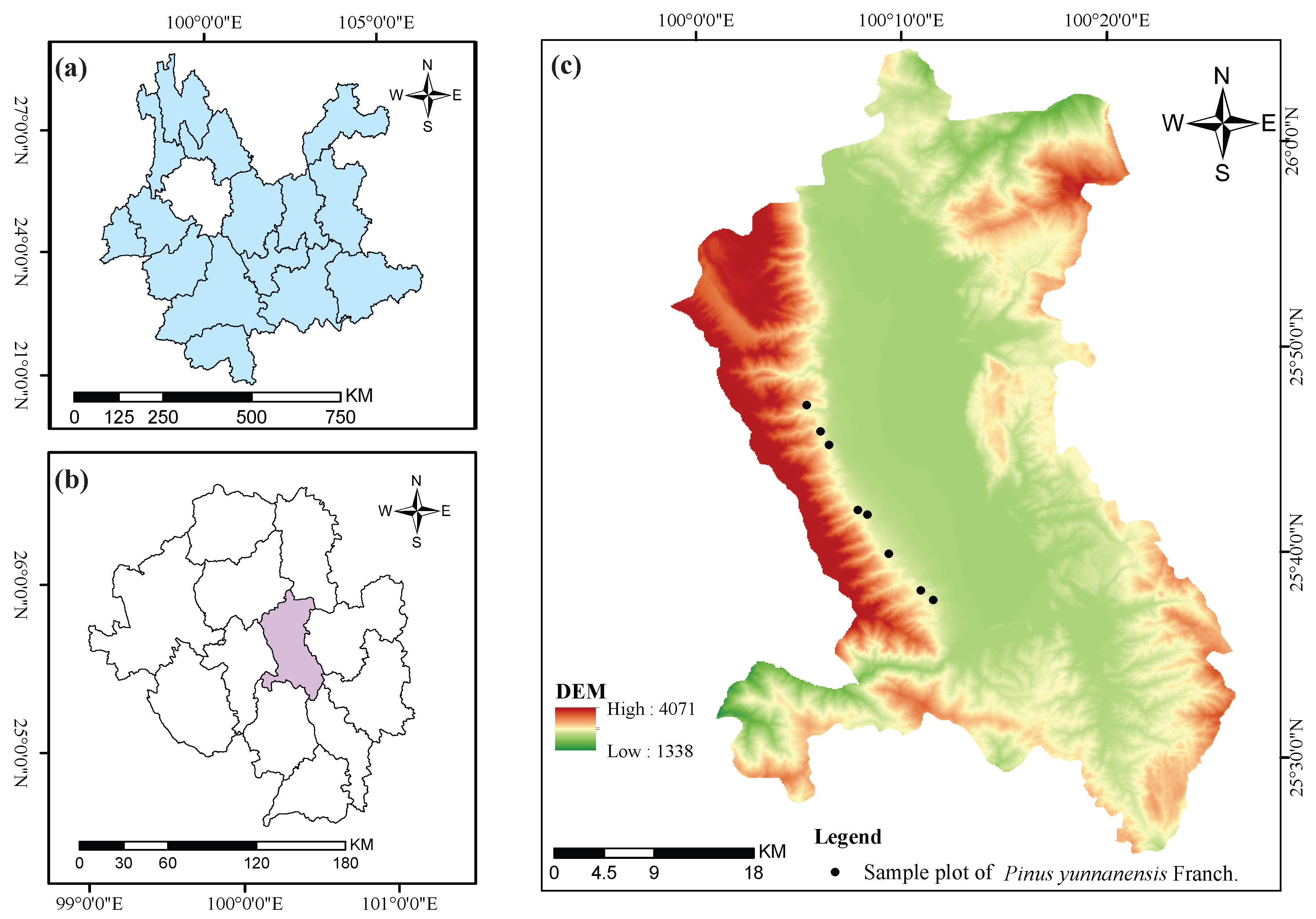
The study area is located on the eastern slope of Cangshan Mountain in Dali City, Yunnan Province, China, with geographic coordinates ranging from 25°25
′ N to 26°02
′ N latitude and 99°58
′ E to 100°27
′ E longitude. The elevation spans from 1966 m to 4122 m. The Cangshan mountain range stretches continuously with 19 major peaks. This region falls under the subtropical plateau monsoon climate, characterized by abundant sunlight, rich heat, minimal interannual climate variation, and distinct wet and dry seasons. The average annual temperature is 16.1 °C, with total annual precipitation reaching 861.6 mm, most occurring between May and October. The climate changes significantly with elevation: areas below 2600 m are classified as mid-subtropical, from 2600 m to 3300 m as mountain temperate climate, and above 3300 m as cold temperate. The forest vegetation in the region is dominated by
Pinus yunnanensis, accompanied by several other species such as
Pinus armandii Franch.,
Betula alnoides Buch.-Ham. ex D.Don,
Vaccinium bracteatum Thunb.,
Ternstroemia gymnanthera (Wight & Arn.) Bedd., and
Gaultheria griffithiana Wight [
35]. The geographic location of the study area is shown in
Figure 1.
2.2. Data Collection
This study utilized data from eight circular permanent sample plots established in
Pinus yunnanensis secondary forests within the study area. Compared to traditional square plots, circular plots are easier to establish and relocate in the field and offer better adaptability to complex terrain [
36]. The initial surveys of these plots were conducted between October 2021 and December 2022, with remeasurements completed between October and December 2024. Detailed information on each plot—including elevation, slope, aspect, radius, and initial survey date—is provided in
Table 1.
Within each plot, individual tree measurements were carried out to record the survival or mortality status and related growth attributes. Summary statistics of tree-level variables are provided in
Table 2. Corresponding climatic data were obtained from the ClimateAP software [
37], based on the survey year and geographic coordinates of each plot. These data include annual and monthly climatic variables, which were subsequently used to calculate seasonal and growing-season averages. In particular, growing-season indicators were derived using temperature and precipitation data from May to October of the respective survey year, representing the biologically active period of
Pinus yunnanensis in the Cangshan region of Dali, Yunnan Province [
38]. Detailed climatic statistics are provided in
Table 3.
2.3. Variable Selection
The candidate predictor variables used in this study were classified into the following five categories: (1) individual tree variables, describing the growth characteristics of each tree, including diameter at breast height (DBH) and its transformations, tree height (TH), and crown width (CW); (2) stand-level variables, representing the structural characteristics of the sample plots, such as basal area per hectare (BA), average diameter at breast height (), and mean dominant tree height (); (3) competition variables, indicating the competitive environment of individual trees, including the cumulative basal area of larger trees (BAL), relative diameter, the ratio of tree DBH to stand basal area (DBA), and the Hegyi competition index; (4) site variables, describing the site conditions of the plots, including elevation, slope, and aspect; (5) climatic variables, covering mean annual temperature (MAT), mean warmest month temperature (MWMT), mean coldest month temperature (MCMT), and mean annual precipitation (MAP).
After identifying the candidate predictor variables, this study performed correlation analysis and variance inflation factor (VIF) tests to screen the variables. First, highly correlated redundant variables within the same category were removed through correlation analysis to avoid information redundancy among multiple variables. Then, VIF tests were applied to detect multicollinearity, and variables with VIF values exceeding 10 were considered to exhibit severe multicollinearity and were eliminated. Through this two-step screening process, the final set of variables for model development was determined. The final predictors retained in the model are presented in the Results section.
2.4. Model Selection
2.4.1. Generalized Linear Model
In current research, the status of mortality as a dependent variable typically does not satisfy the assumption of normal distribution. As a result, Generalized Linear Models (GLM) have been widely applied to analyze the probability of tree mortality and survival, becoming one of the most commonly used methods for tree mortality prediction [
7,
39]. When the GLM employs a logit link function, it forms a logistic regression model. One of the key advantages of this model is that its predicted values are constrained between 0 and 1, making it particularly suitable for modeling the natural probability of tree mortality. Given that mortality is a typical binary event, the logistic model effectively characterizes the survival and mortality status of trees and evaluates mortality risk through predicted probabilities: the closer the predicted value is to 1, the higher the likelihood of mortality; conversely, lower values indicate a greater probability of survival. In this study, we employed the logistic model to construct an individual tree mortality model for
Pinus yunnanensis secondary forests. The model was implemented using the “LogisticRegression” function from the “sklearn.linear model” module in Python 3.11, and its general mathematical form is expressed as follows:
where
i and
j represent the
tree within the
plot,
denotes the matrix of independent variables, the superscript
T indicates the transpose of a vector,
represents the vector of model parameters,
is the model’s error term, and
refers to the probability of tree survival or mortality.
2.4.2. Generalized Linear Mixed-Effects Model
The GLMM extends the GLM by incorporating random effects to account for variability across different hierarchical levels of the data structure [
40]. Since the tree mortality data used in this study were collected from repeated surveys across different sample plots, the dataset naturally forms a three-level hierarchical structure, with individual trees nested within plots and plots nested within regions. By applying the mixed-effect model, it becomes possible not only to accurately analyze the influence of various explanatory variables on tree mortality but also to enhance the predictive accuracy of the mortality model. Preliminary comparisons indicated that, under the condition of statistically significant fixed effects, there was no notable difference in model performance between including both plot- and region-level random effects and including only plot-level random effects. Therefore, this study adopted a GLMM that includes only the plot-level random effects. The model was implemented using the “pymer4” package in Python 3.11. The corresponding model formulation is given below:
where
and
represent the design matrices for fixed effects and random effects, respectively; the superscript
T indicates the transpose of a vector,
is the vector of fixed-effect parameters;
is the vector of random-effect parameters;
D denotes the variance-covariance matrix of the random effects; and
is the error term of the model.
2.4.3. Random Forest
Random Forest, originally proposed by Breiman [
41], is an ensemble learning algorithm that enhances model robustness and generalization by aggregating the outputs of multiple independently generated decision trees. This approach employs bootstrap resampling of the training data and random selection of feature subsets during each tree’s construction, thereby mitigating the overfitting issues commonly associated with individual decision trees. Moreover, RF inherently assesses variable importance by quantifying each predictor’s contribution to overall model performance across all splits, enabling the identification of critical factors influencing individual tree mortality risk. In this study, the RF model was developed and its hyperparameters were tuned using the “RandomForestClassifier” package within the Python computing environment. To identify an appropriate balance between model complexity and predictive performance, hyperparameter tuning was conducted via five-fold cross-validated grid search. The number of trees (n_estimators) was tested from 100 to 1000 in increments of 100, while the number of features considered at each split (max_features) was varied from 1 to 10.
2.4.4. Support Vector Machine
Support Vector Machine is a single machine learning algorithm that uses a single decision boundary to classify data [
42]. It operates by constructing an optimal separating hyperplane within the sample space that maximizes the margin between classes, thereby effectively partitioning complex data structures. For nonlinear relationships, SVM leverages kernel functions to project input features into a high-dimensional space, enhancing its capacity to fit intricate decision boundaries. SVM is particularly advantageous in scenarios characterized by limited sample sizes and high-dimensional feature spaces, as the model complexity and generalization performance can be flexibly controlled by adjusting the penalty parameter (C) and kernel parameters (e.g., gamma). In this study, the SVM model was trained and its hyperparameters were optimized using the “SVC” package in the Python computing environment. The penalty parameter (C) varied from 0.1 to 10, while the kernel coefficient (gamma) was evaluated at discrete values ranging from 0.001 to 0.1. For the linear kernel, no kernel-specific parameters were required; for the RBF kernel, gamma served as the main parameter controlling model complexity; and for the polynomial kernel, the degree was fixed at its default value of 3.
2.4.5. Extreme Gradient Boosting
Extreme Gradient Boosting is an efficient boosting algorithm based on the Gradient Boosting Decision Tree (GBDT) framework [
43], and it is an ensemble learning method that combines the predictions of multiple decision trees in a boosting manner to improve model accuracy and robustness. It iteratively trains multiple decision trees, continuously optimizing the loss function while incorporating regularization terms to control model complexity and prevent overfitting. In each training round, XGBoost computes the negative gradients of the samples to fit the residuals and significantly accelerates model construction by utilizing a parallelized split-point search technique. Ultimately, the model aggregates the weights corresponding to the leaf nodes across all trees to generate the final prediction. In this study, XGBoost was applied to predict the probability of individual tree mortality, leveraging its superior computational efficiency and nonlinear modeling capabilities. Both the model construction and hyperparameter tuning were implemented using the “xgboost” package in Python 3.11. A five-fold cross-validated grid search was employed to optimize the model. The learning rate (shrinkage) was set to vary between 0.001 and 0.1, the number of trees was tested at 100, 500, and 1000, and the maximum tree depth was adjusted across values of 1, 3, 5, 7, and 9.
2.4.6. Stacking Ensemble Learning Algorithm
Stacked Generalization, also known as stacking, is an ensemble method that combines the predictions of multiple base learners as inputs to a meta-learner for the final prediction [
28]. The core principle behind stacking is to leverage the strengths of each base learner on different data features, thereby reducing the bias and variance of individual models and improving overall prediction performance. Stacked ensemble methods typically involve two main steps: first, training multiple base learners, where each learner independently learns from the training data and generates its predictions; second, using these predictions as new features to train a meta-learner, which makes the final prediction based on the outputs of the base learners. By combining different types of base models, stacked generalization can better capture complex patterns in the data, enhancing the robustness and stability of the model. This method has significantly improved performance, especially when dealing with high-dimensional and complex data.
In this study, we use Random Forest, SVM, and XGBoost as base learners, and Logistic Regression as the meta-learner. Specifically, we first train Random Forest, SVM, and XGBoost on the training data and generate their respective predictions. Then, these predictions are used as features to train the Logistic Regression model, which produces the final prediction. All base learners were tuned using predefined hyperparameter ranges prior to integration, and their optimal configurations were used to construct the final stacked model.
2.5. Threshold Optimization
Optimizing the classification threshold is a critical issue in constructing individual tree mortality models, and it directly influences model performance. An appropriately optimized threshold is essential for effectively distinguishing between deceased and surviving trees; a threshold set too high may result in missed detections (i.e., false negatives), while one set too low may lead to false alarms (i.e., false positives). Thus, scientifically and reasonably optimizing the threshold is central to ensuring both high accuracy and reliability in practical applications.
Current approaches for threshold determination primarily include fixed threshold, Mistake Classification Rate (MCR) minimization, MST, and Kappa coefficient methods [
33]. Based on empirical knowledge or domain expertise, the fixed threshold method, is simple to implement but lacks flexibility and may not adapt well to different datasets. The MCR minimization method optimizes the threshold by minimizing the overall classification error, making it suitable for balanced datasets. The MST method achieves a balance between sensitivity and specificity, which is beneficial in scenarios where controlling both error types is critical. In contrast, the Kappa coefficient method optimizes the threshold by maximizing the Kappa statistic—a measure of agreement between predicted and true classifications—thus being particularly effective for imbalanced datasets [
44].
This study additionally incorporates a curve-based approach, the PR curve method, to enhance threshold optimization and model performance. By plotting the precision-recall (PR) curve, calculating the area under the PR curve (AUPRC), and selecting the threshold that yields the best balance between precision and recall [
34], the PR curve method is especially suited to imbalanced datasets and more accurately reflects model performance on the minority class (i.e., dead trees).
Ultimately, in this study, four threshold optimization methods were employed to determine the optimal threshold for the individual tree mortality model: MCR minimization, MST, Kappa coefficient, and PR curve. For each method, candidate thresholds ranging from 0 to 1 with a step size of 0.01 were systematically evaluated based on their corresponding optimization criteria—minimizing classification error for MCR, maximizing separation for MST, maximizing the Kappa coefficient, and maximizing the F1 score for the PR curve. Based on these evaluations, the optimal threshold for each model was initially identified.
In addition, given the variation in optimal thresholds produced by different methods, a scoring-based strategy was further adopted to determine the final threshold for each model. Specifically, for each candidate threshold, six evaluation metrics—accuracy, recall, true negative rate, F1 score, Kappa coefficient, and MCR—were calculated. For each metric, the performance values of all candidate thresholds were ranked: higher values of accuracy, recall, true negative rate, F1 score, and Kappa coefficient were assigned higher ranks (i.e., descending order), while lower MCR values were assigned higher ranks (i.e., ascending order). The ranks each threshold received across all six metrics were then summed to produce a total score, and the threshold with the lowest total score was selected as the final optimal threshold. Subsequently, performance metrics were recalculated under each final threshold to enable comprehensive model comparison.
2.6. Model Evaluation
The dataset in this study was partitioned using an 8:2 split ratio, with 80% of the original data used for training the model parameters and 20% reserved as a test set to evaluate the predictive performance of the models. All performance evaluation metrics for the individual tree mortality models include AUC, accuracy, recall, TNR, MCR, F1 score, and Kappa coefficient [
45]. Additionally, since the baseline model employed in this study is a binary logistic model, on which a plot-level single random effect mixed model was subsequently built, the Akaike Information Criterion (AIC) was used to compare the performance of the baseline model with that of the mixed-effect model. The specific formulations of all evaluation metrics are as follows:
where
denotes the number of samples correctly predicted as positive,
denotes the number of samples incorrectly predicted as positive,
denotes the number of samples correctly predicted as negative,
denotes the number of samples incorrectly predicted as negative,
L represents the maximum likelihood value of the model, and
K denotes the number of model parameters.
3. Results
After a rigorous screening of candidate explanatory variables, the following predictors were retained in the
Pinus yunnanensis individual tree mortality model: the square of DBH, TH, the Hegyi competition index, DBA,
, aspect, slope, elevation,
, MAT, and MAP. In the final model, the VIF for all predictors was less than 10, thereby indicating the absence of substantial multicollinearity. The estimated model coefficients, as detailed in
Table 4, are all statistically significant (
p < 0.05).
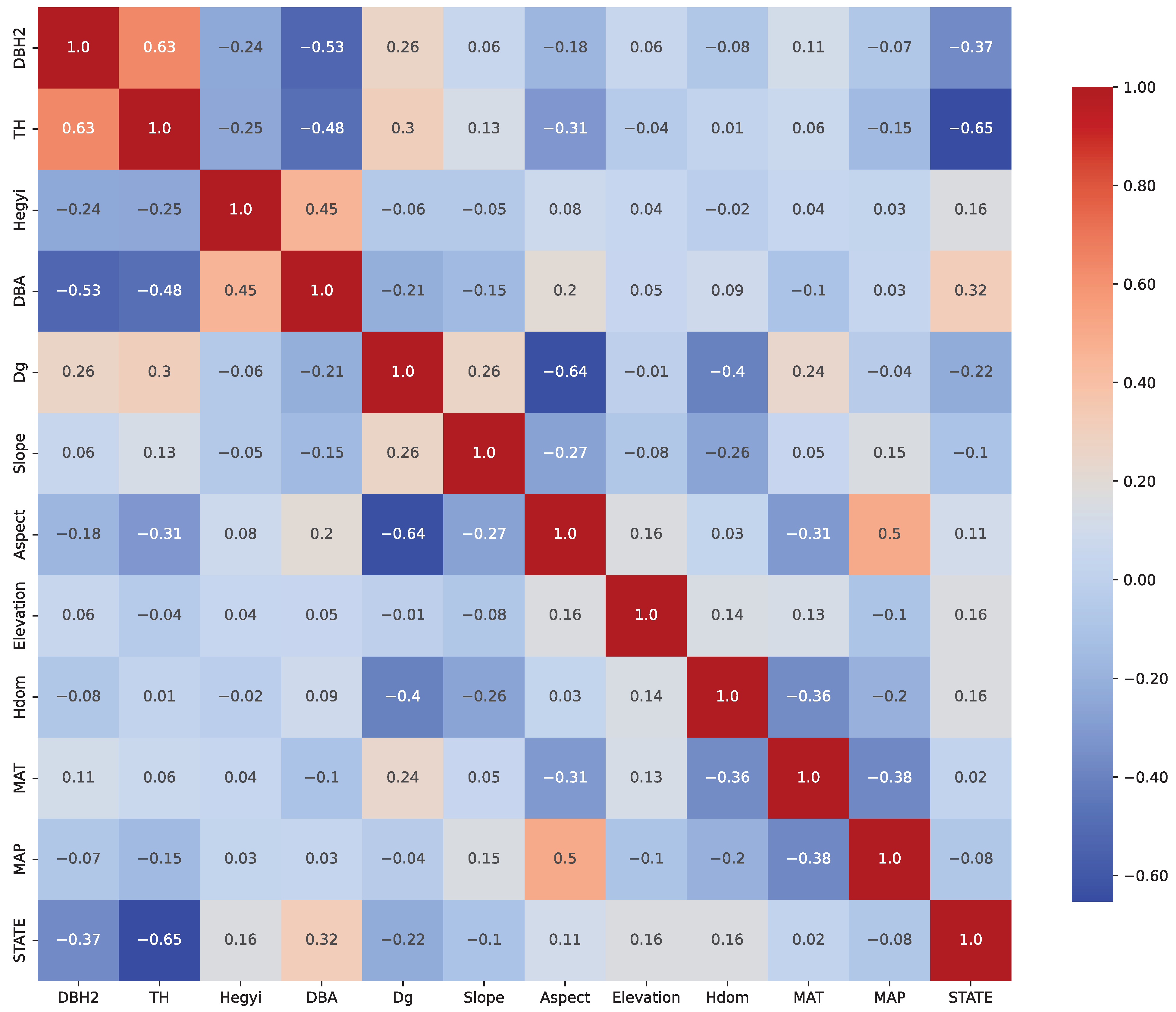
Figure 2 shows the Pearson correlation matrix of the selected predictors, indicating that multicollinearity was not present after variable selection.
Based on these results, the model can be formally represented as follows:
where,
to
are the parameters to be estimated, with the estimation results presented in
Table 4.
According to the signs of the estimated parameters in
Table 4, DBH, tree height, the ratio of DBH to stand basal area, aspect, and mean annual precipitation are negatively correlated with the probability of tree mortality, In contrast, the the Hegyi competition index, stand mean diameter, slope, elevation, dominant tree height, and mean annual temperature positively correlate with mortality probability. Specifically, larger DBH, greater tree height, and a higher ratio of DBH to stand basal area are associated with a lower probability of tree mortality, whereas higher competition intensity increases the likelihood of mortality. In addition, increases in aspect and mean annual precipitation reduce the probability of mortality, while increases in slope, elevation, dominant tree height, and mean annual temperature lead to a higher probability of mortality.
Based on the Generalized Linear Model, a Generalized Linear Mixed-Effect Mortality Model is established by incorporating plot-level random effects. The specific form of the model is as follows:
where,
represents the random effect parameter, while the meanings of the other variables remain the same as in the Generalized Linear Model.
The parameter estimates and the variance structure of the random effects are presented in
Table 4. The signs of the parameter estimates in the mixed-effects model are consistent with those in the base model, and the results are biologically meaningful. As shown by the evaluation metrics in
Table 4, the inclusion of plot-level random effects in the base model led to improvements in performance metrics such as AUC and accuracy, along with a reduction in AIC, indicating an enhancement in model fit. These results further demonstrate that incorporating plot-level random effects can improve the overall model performance.
Compared with traditional models, this study’s machine learning models also used the same variables selected through variable selection, with the dependent and independent variables consistent with those in traditional statistical models. Additionally, compared with traditional models, this study’s machine learning models also used the same variables selected through variable selection, with the dependent and independent variables consistent with those in traditional statistical models. The optimal hyperparameters obtained through grid search were as follows: 300 trees and 6 features per split for Random Forest; C = 10, and an RBF kernel with gamma = 0.1 for SVM; and a learning rate of 0.1, 500 trees, and maximum depth of 5 for XGBoost. All performance metrics reported in
Table 5 were derived using these optimized settings with a fixed classification threshold of 0.5. Furthermore, the Stacked-RSX model was constructed based on these individually optimized base learners to ensure consistent and fair model comparison.
The table results indicate that traditional statistical models for tree mortality (GLM and GLMM) perform worse across all metrics compared to machine learning-based models, with lower accuracy, recall, and true negative rates, and higher misclassification rates. The Random Forest model shows significant improvements in accuracy and recall, with a higher true negative rate and a notable decrease in misclassification rate, reflecting better differentiation between positive and negative samples. The Support Vector Machine model excels in recall but still lags behind Random Forest and XGBoost in overall performance.
Notably, the Stacked-RSX model demonstrates superior performance across all metrics, especially in accuracy (0.8902), recall (0.8688), and F1 score (0.8750), outperforming other models and further enhancing the overall performance of mortality prediction. The analysis results indicate that machine learning models significantly improve the performance of tree mortality prediction tasks, and the Stacked-RSX model, with its outstanding overall capability, emerges as the best prediction model.
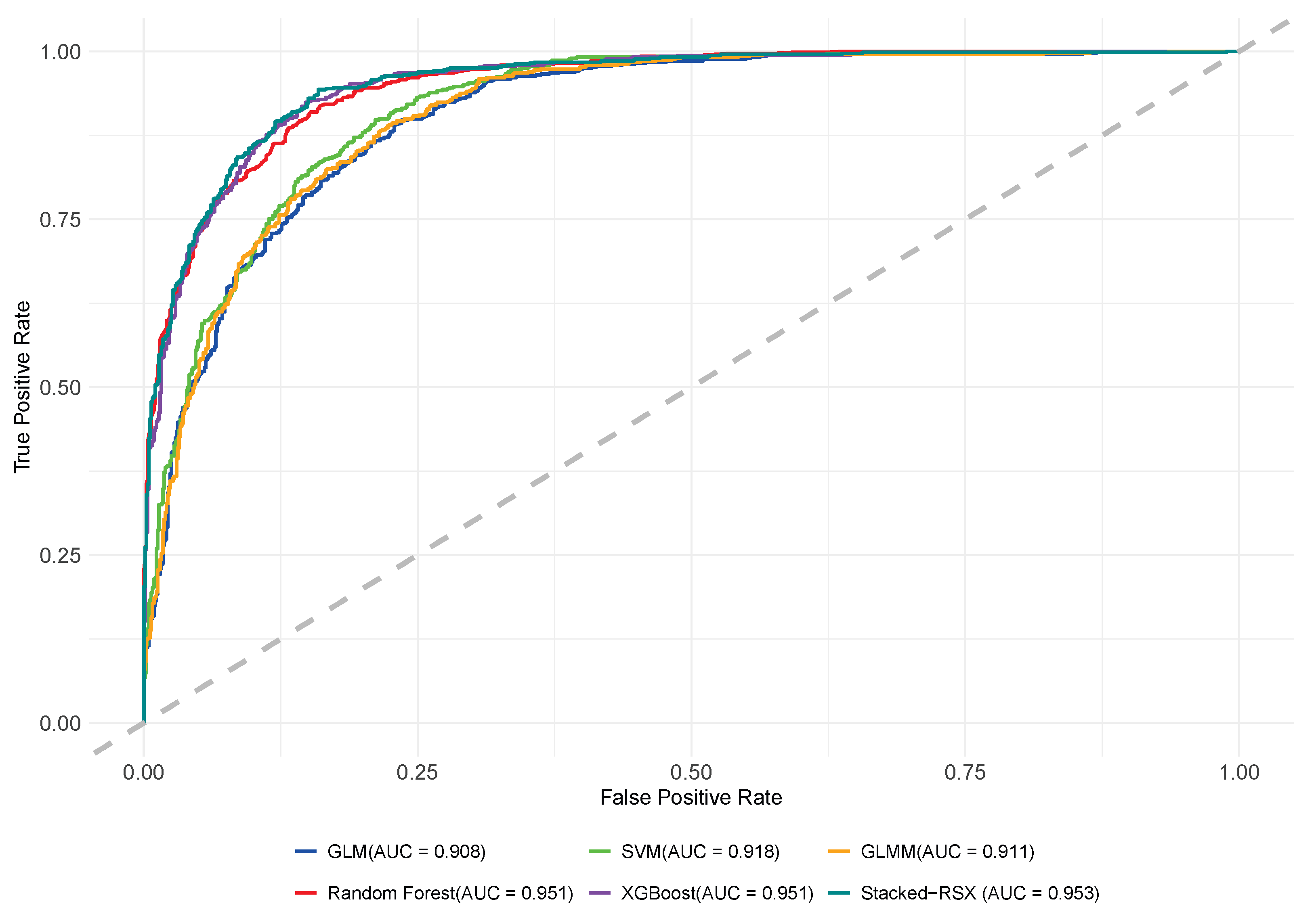
As shown in
Figure 3, the ROC curve results highlight differences in classification performance across models for individual tree mortality prediction. XGBoost and Random Forest achieved an AUC of 0.951, demonstrating excellent ability to distinguish between live and dead trees with high true positive rates and low false positive rates. GLMM and SVM had AUC values of 0.911 and 0.918, respectively, showing improvement with random effects or nonlinear boundaries, but still slightly underperformed compared to XGBoost and Random Forest. GLM, with an AUC of 0.908, showed weaker predictive ability, indicating limitations in handling data complexity and variable interactions. Notably, the Stacked-RSX model outperformed all others with an AUC of 0.953, confirming the strength of stacking ensemble models in predicting tree mortality. Overall, ensemble-based models (XGBoost, Random Forest, and Stacked-RSX) showed the best performance, demonstrating strong adaptability and generalization. GLMM and SVM, as secondary choices, provided stable predictions, while GLM, with stricter assumptions, slightly lagged in classification ability.
3.1. Analysis of Threshold Optimization
A comparative analysis of the different threshold optimization methods revealed that the optimal thresholds determined by the MCR minimization and Kappa coefficient methods were generally consistent across most models. In contrast, the thresholds derived from the PR curve method led to significantly improved model performance. Notably, for the Stacked-RSX and XGBoost models, thresholds optimized by the PR curve method yielded superior results in key evaluation metrics, including accuracy, recall, true negative rate, and F1 score, thereby enhancing overall predictive effectiveness. Importantly, these lower thresholds were more effective in identifying mortality cases and substantially reduced the likelihood of misclassifying dead trees as alive, which is critical for practical forest management applications.
Based on this integrated ranking approach, the final optimal thresholds were determined as follows: 0.36 for the base and mixed-effects models, 0.41 for Random Forest, 0.29 for SVM, 0.35 for XGBoost, and 0.25 for the Stacked-RSX model. After determining the optimal threshold,
Table 6 presents the evaluation metrics for each model at its corresponding optimal threshold. The metrics in the table reveal that the XGBoost model exhibits outstanding performance across key indicators such as accuracy, recall, and true negative rate, while also achieving the lowest misclassification rate along with high F1 score and Kappa coefficient. This indicates that XGBoost has a significant advantage in aligning its predictions with the true labels, resulting in the best overall performance. The Random Forest model also performs well; its high accuracy and true negative rate reflect strong stability and reliability in distinguishing between positive and negative samples. The Support Vector Machine model, though it demonstrates excellent recall—indicating a strong ability to identify positive samples—lags slightly behind XGBoost and Random Forest in overall performance. In contrast, the traditional statistical models (GLM and GLMM) show relatively lower performance in terms of accuracy, F1 score, and Kappa coefficient. Although the GLMM model offers some improvement over GLM, neither traditional model approaches the performance level of the machine learning models. Overall, these results indicate that machine learning-based models deliver higher predictive accuracy and comprehensive performance, whereas traditional statistical models exhibit certain limitations.
3.2. Analysis of Feature Importance
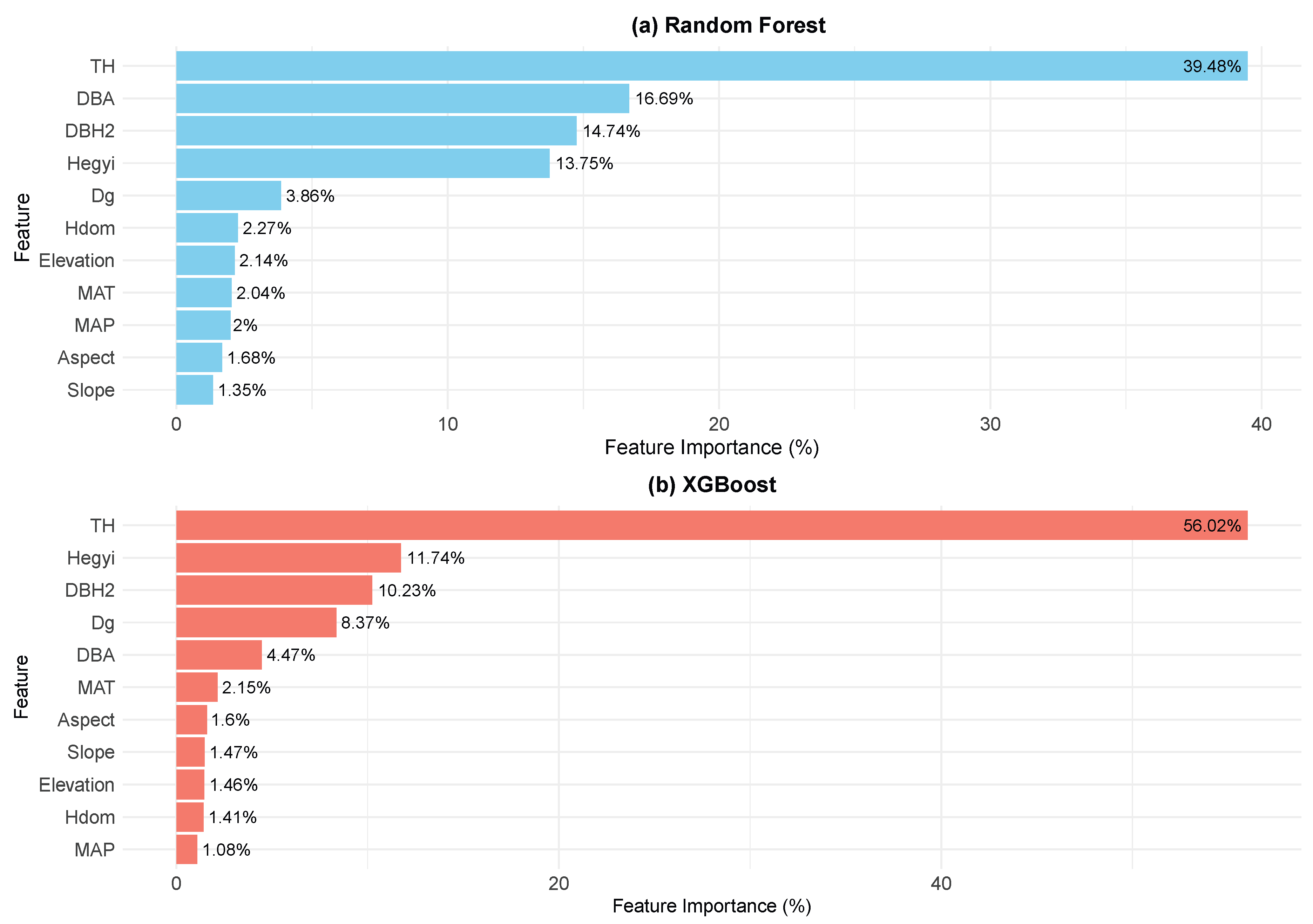
The feature importances shown in
Figure 4 were derived from the feature_importances_ attribute of the XGBoost and Random Forest models. As shown in
Figure 4, intrinsic factors and competition indices play dominant roles in predicting individual tree mortality. Notably, tree height is highly influential, with importance values of 56.02% in XGBoost and 39.48% in Random Forest, indicating that its effect on mortality probability far exceeds that of other variables and serves as a key determinant of tree survival. Additionally, the transformed form of DBH exhibits importance values of 10.23% in XGBoost and 14.74% in Random Forest, demonstrating that DBH also significantly affects mortality, with smaller-diameter trees being more susceptible, thereby underscoring the role of overall growth status in prediction.
Competition indices similarly contribute substantially to mortality probability. The Hegyi competition index shows importance values of 11.74% and 13.75% in XGBoost and Random Forest, respectively, highlighting that the competitive pressure experienced by an individual tree is a major determinant of its survival probability; higher competition leads to higher mortality risk. Moreover, the ratio of DBH to stand basal area is deemed important, with values of 4.47% in XGBoost and 16.69% in Random Forest, suggesting that an individual tree’s relative position within the stand has a significant impact on its mortality risk. Specifically, trees with higher DBH-to-basal area ratios likely occupy more favorable positions, thereby accessing more resources and enjoying a survival advantage, whereas those with lower ratios tend to experience greater competition pressure and, consequently, a higher likelihood of mortality.
In contrast, the effect of stand-level factors on mortality is relatively limited. The average stand DBH has importance values of 8.37% in XGBoost and 3.86% in Random Forest, indicating that while it does influence individual tree mortality, its effect is comparatively weak. Furthermore, the mean dominant tree height in the models does not exceed 2.5% in importance, further demonstrating that stand-level factors have a minor role in predicting mortality. This may be because, in comparison to intrinsic traits and competition pressure, the overall growth status of the stand exerts a less direct impact on an individual tree’s likelihood of mortality.
Additionally, the importance of site factors (slope, aspect, and elevation) is consistently low in both models, with the highest value not exceeding 2.5%. This suggests that topographical conditions have a limited impact on mortality—likely due to relatively stable terrain conditions that do not impose significant environmental stress. Climate factors also have a minimal effect, with mean annual temperature and annual precipitation exhibiting maximum importance values of approximately 2%. This indicates that, within this study, climate exerts only a slight direct influence on mortality probability.
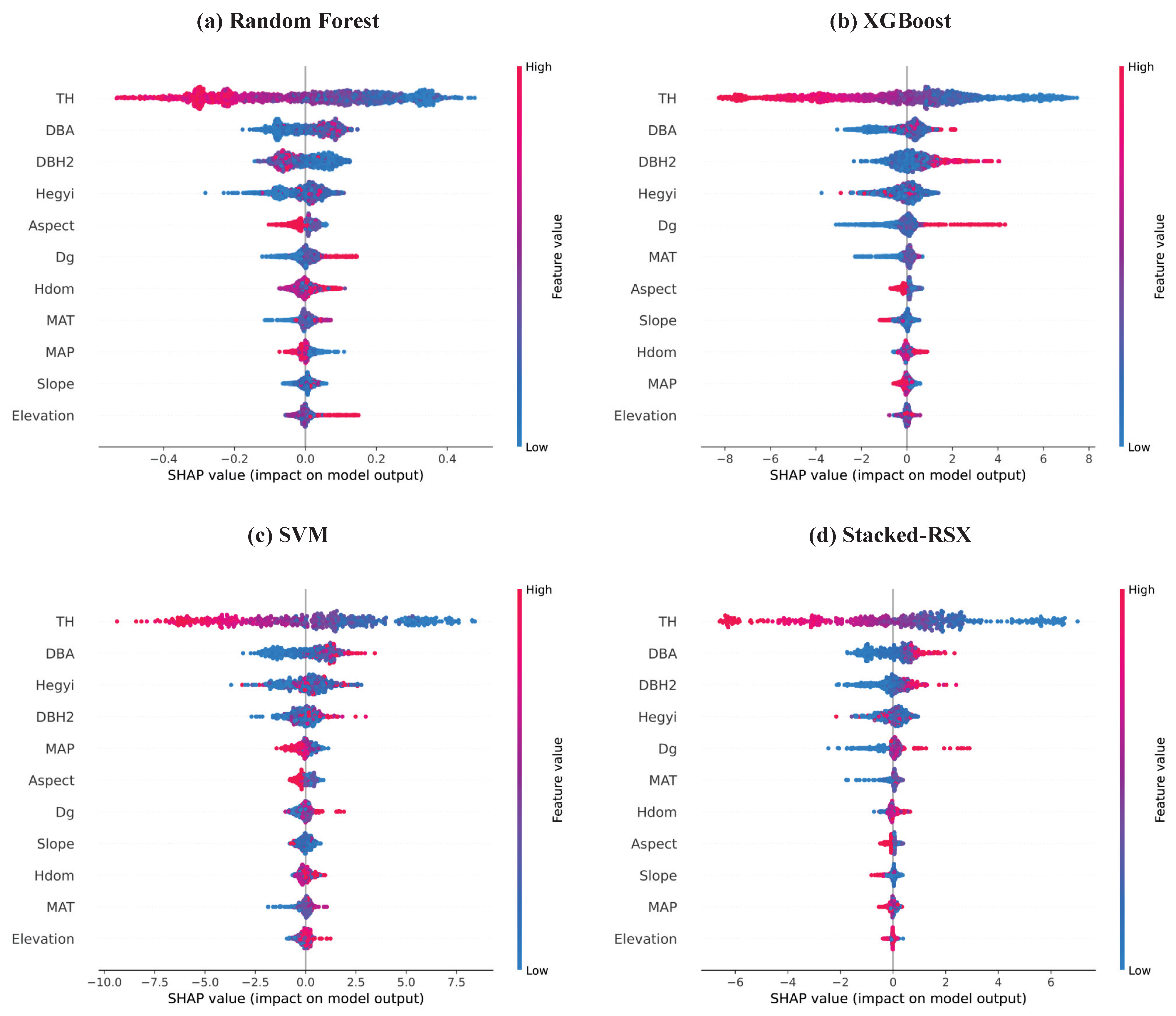
Figure 5 shows the SHAP summary plots generated by four models (Random Forest, XGBoost, SVM, and Stacked-RSX) for predicting tree mortality. SHAP assigns each feature an importance value based on its average contribution to the model’s output across all predictions, grounded in cooperative game theory. The results of the feature importance analysis are consistent with the previous analysis, further confirming the role of various factors in predicting the mortality risk of
Pinus yunnanensis.
As shown in
Figure 5, TH is negatively correlated with mortality risk, indicating that taller trees are generally associated with a lower mortality risk, whereas shorter trees tend to have a higher probability of dying. In contrast, DBA is positively correlated with mortality risk across all models. Higher DBA values are typically associated with lower mortality risk, suggesting that trees with a better relative growth position in the stand are able to access more resources, thus reducing the mortality risk.
is positively correlated with mortality risk in the XGBoost, SVM, and Stacked-RSX models, meaning that larger DBH values, which typically indicate older trees, are linked to a higher mortality risk. However, in the Random Forest model,
is negatively correlated with mortality risk, suggesting that larger DBH values are associated with a lower mortality risk. This indicates that different models handle the nonlinear relationship between DBH and mortality risk differently.
Moreover, the Hegyi competition index is positively correlated with mortality risk in all models. As the competition index increases, the mortality risk also rises, reflecting that higher competition among trees limits their growth, thus increasing the likelihood of mortality. Similarly, is positively correlated with mortality risk, indicating that a larger value typically means a more mature stand, where increased resource competition raises the mortality risk. also shows a positive correlation with mortality risk, as a higher indicates more intense competition within the stand, restricting tree growth and increasing the risk of mortality.
In addition, MAP is negatively correlated with mortality risk, suggesting that higher rainfall usually helps trees obtain sufficient water and nutrients, enhancing their resistance to stress and reducing the likelihood of mortality. Conversely, MAT is positively correlated with mortality risk, indicating that stands with higher average temperatures are associated with increased mortality risk.
Finally, Aspect and Slope are both negatively correlated with mortality risk, suggesting that certain aspects and slopes in the study area provide more favorable growing conditions, thereby reducing the mortality risk. Elevation is positively correlated with mortality risk, with higher elevations associated with higher mortality risks, likely due to harsher climatic conditions and growing pressures at higher altitudes. However, the effects of these three factors on mortality risk are relatively minor and do not play a decisive role in predicting tree mortality.
4. Discussion
This study used five models (GLM, GLMM, Random Forest, SVM, and XGBoost) to construct an individual tree mortality prediction model for
Pinus yunnanensis, and their performance was compared using a fixed threshold of 0.5. Because the modeling data were derived from re-surveyed permanent sample plots, the dataset exhibits high autocorrelation and a hierarchical structure. Incorporating random effects allows for a better capture of the correlations among repeated measurements within the same plot [
19], thereby avoiding potential biases that may arise in GLM from assuming independent observations. In addition, the heterogeneity among plots cannot be fully explained by fixed effects alone, and random effects provide a flexible means to account for this unobserved variability, thereby enhancing model fit and the reliability of inferences. Moreover, including random effects enables more accurate estimation of standard errors and reduces the risk of false positives due to neglected within-group correlations. The final results indicate that the logistic mixed-effect model at the plot level outperforms the baseline logistic model regarding classification performance.
Compared to traditional statistical models (GLM and GLMM), machine learning models exhibit greater flexibility and adaptability in handling data autocorrelation. Traditional mixed effects models heavily rely on predefined autocorrelation structures [
46], but real-world repeated measures data often exhibit nonlinear spatiotemporal characteristics that fixed covariance structures cannot effectively capture. In contrast, machine learning models possess strong nonlinear expression capabilities, enabling them to automatically identify and utilize local patterns and complex interactions in the data without assuming any predefined autocorrelation structure. Therefore, even in the presence of autocorrelation, machine learning models can effectively extract information from the data in a data-driven manner [
47].
Additionally, ensemble learning models, such as Random Forest and XGBoost, build multiple decision trees and fully exploit local correlations between samples during the feature splitting process, thus reducing errors and biases induced by autocorrelation. This gives these models a distinct advantage over traditional statistical models when dealing with complex, autocorrelated data [
30]. As a result, machine learning methods generally perform better than traditional GLM and GLMM models in individual tree mortality models. Furthermore, compared to traditional machine learning methods and single ensemble learning approaches, stacking ensemble models integrate the different characteristics of multiple base learners, allowing each model to leverage its strengths under different data patterns [
48,
49]. By combining the base learners through a meta-learner, stacking ensemble models reduce the risks of overfitting or underfitting that may arise from using a single model [
28]. This multi-level, data-driven combination approach enables stacking ensemble models to provide more robust and precise predictions in high-dimensional and complex interaction scenarios. Moreover, stacking ensemble methods can effectively mitigate the limitations of individual base learners, such as the computational bottlenecks SVM may face in high-dimensional data, or the performance fluctuations of Random Forest under specific patterns, thereby improving the model’s overall stability and generalization ability.
However, stacked ensemble models also have certain drawbacks and considerations. First, they require more computational resources, especially when training multiple base models and a meta-model, which results in more time and resource consumption. In Addition, when the base models already perform well, the performance improvements from stacking tend to diminish. As the base models improve, the incremental gains from stacking become relatively limited, and improvements in core metrics like accuracy may become marginal [
50]. Therefore, it is important to strike a balance between performance enhancement and the added computational cost and system complexity. A balance must be struck between improving model performance, managing computational resource consumption, and minimizing deployment complexity to ensure efficiency while avoiding unnecessary resource waste and increased complexity.
Since the individual tree mortality model outputs predicted probabilities that require a threshold to determine whether a tree is dead or alive, selecting an appropriate threshold is crucial. Although numerous threshold determination methods have been proposed [
33], there is no universally accepted best method. In this study, we employed four approaches—MCR minimization, MST method, Kappa coefficient method, and PR curve method—to determine the threshold for the individual tree mortality model. The classification accuracies of the different models were then compared based on the determined thresholds. As shown in
Table 6, the MCR minimization method generally yielded higher accuracy and true negative rate across all models. However, its drawback lies in a lower recall, indicating a deficiency in positive class recognition. In contrast, the MST method achieved a balance between true negative rate and recall, rendering the model more balanced in its classification capability, although it may not attain optimal overall performance. The Kappa coefficient method, which emphasizes the balance of the classifier by maximizing the Kappa coefficient to ensure equilibrium between survival and mortality classifications, generally achieved satisfactory performance. Notably, the PR curve method consistently produced the best results among all models. This is attributable to the PR curve’s focus on balancing precision and recall, making it particularly suitable for imbalanced datasets. By optimizing the classification threshold based on the PR curve, the model effectively improved recall and, consequently, its ability to identify positive (mortality) cases [
34]. Therefore, the preliminary results of this study indicate that, based on the scoring and ranking of all evaluation indicators, the PR curve method is the most effective threshold determination approach for the individual tree mortality models employed in this study.
Based on the explanatory results of the parameter estimation of the statistical model, the built-in methods of the machine learning model, and the SHAP method, both DBH and tree height exhibit very high importance. In particular, as DBH and tree height increase, the probability of individual tree mortality tends to decrease. However, many studies have indicated that when DBH is relatively small, intense competition leads to a higher likelihood of mortality; as trees continue to grow, their competitive ability improves, resulting in a reduced mortality probability; yet, once DBH increases beyond a certain threshold, trees enter an aging stage, and mortality probability begins to rise, forming a U-shaped relationship between DBH and mortality [
5,
51]. The negative coefficient for DBH in the statistical models indicates that the mortality probability of
Pinus yunnanensis decreases with increasing DBH. However, this does not capture the eventual increase in mortality due to senescence. This discrepancy is likely attributable to the fact that the
Pinus yunnanensis secondary forests in the current study area are primarily in the juvenile to near-mature stages. Additionally, tree height is highly correlated with mortality probability in
Pinus yunnanensis. As indicated by the feature importance proportions in
Figure 4, the contribution of tree height to mortality prediction exceeds 35%.
Both DBH and tree height generally indicate that a tree is in a competitive advantage position. Analysis of individual tree factors suggests that competition indices are one of the direct determinants of tree mortality [
10,
52]. In this study, the overall contributions of the competition factors—specifically, the Hegyi competition index and the ratio of DBH to stand basal area—exceeded 15 percent, and in the Random Forest model, they surpassed 30 percent. Notably, the parameter estimate for the DBH-to-stand basal area ratio is negative, while that for the competition index is positive. This finding aligns with conventional understanding: a larger DBH-to-stand basal area ratio indicates a competitive advantage and is associated with a lower mortality probability, whereas a higher competition index reflects competitive disadvantage and correlates with an increased mortality probability.
In addition, stand factors, site factors, and climatic factors influence on tree mortality [
52], though their impact is limited, despite being statistically significant for tree mortality. Specifically, slope aspect and annual precipitation negatively correlate with tree mortality, indicating that increases in these factors reduce the likelihood of mortality. In this study, all sample plots are located in the Northern Hemisphere, with slope aspects ranging from northeast to southeast, corresponding to values between 45 and 180 degrees. This suggests that as the slope aspect shifts from shaded to sunlit, the risk of tree mortality decreases. Conversely, increases in slope, elevation, dominant tree height, and mean annual temperature contribute to higher tree mortality. Higher slope values may cause trees to grow in steeper environments, making it more difficult to access water and nutrients, which increases growth stress and mortality risk. Conversely, elevation represents harsher growing conditions, limiting the growth of
Pinus yunnanensis and increasing mortality risk [
53]. Higher dominant tree height reflects greater competition within the stand, restricting tree growth and increasing mortality probability [
54]. Additionally, increased mean annual temperature may intensify water evaporation, further increasing tree growth burdens and mortality risk [
55]. These factors collectively limit tree growth and elevate mortality risk, though their effects are less pronounced.
5. Conclusions
This study used two traditional statistical methods (GLM and GLMM) along with three machine learning algorithms (RF, SVM, and XGBoost), combined with a stacking ensemble approach, to develop an individual tree mortality model for Pinus yunnanensis. The results show that the stacking ensemble model (Stacked-RSX) outperforms both single machine learning models and traditional statistical methods in accuracy prediction for individual tree mortality classification. Moreover, machine learning models generally perform better than traditional statistical models in this task. Various interpretability analysis methods further identified TH, DBH, and competition factors as key variables affecting mortality risk. In particular, TH emerged as the most significant factor influencing individual tree mortality probability in Pinus yunnanensis secondary forests. Although the contribution of climate factors is relatively small, they still provide valuable insights into environmental influences.
The study applied several methods to improve classification performance in terms of threshold optimization. The results show that the PR curve optimization method consistently outperformed other methods, significantly enhancing the model’s accuracy in mortality classification.
In conclusion, the research validated the effectiveness of stacking ensemble learning and machine learning methods in improving the accuracy of individual tree mortality classification. Through in-depth model interpretability analysis, the contribution and impact of each feature on the model’s classification results were understood, providing a theoretical foundation for the sustainable management of Pinus yunnanensis forests.
Nevertheless, certain areas remain in need of improvement in this study. Firstly, the current modeling only utilizes variables available from existing field surveys and climatic data, which may not fully capture other ecological factors influencing tree mortality. Secondly, the imbalance in the dataset between live and dead trees might have affected the model’s predictive performance. Future research could benefit from incorporating long-term monitoring data, integrating more comprehensive environmental and biological variables, and exploring advanced algorithms or ensemble approaches to further enhance the accuracy and generalizability of individual tree mortality prediction.


