
L2: Accurate Forestry Time-Series Completion and Growth Factor Inference


Abstract
1. Introduction
- We propose the completion model, which integrates low-rank tensor completion (LRTC) with long short-term memory (LSTM) networks to enhance the completeness and accuracy of forestry time-series data. This model effectively optimized and completed time-series data for Populus tomentosa forest farms, significantly improving data integrity and reliability.
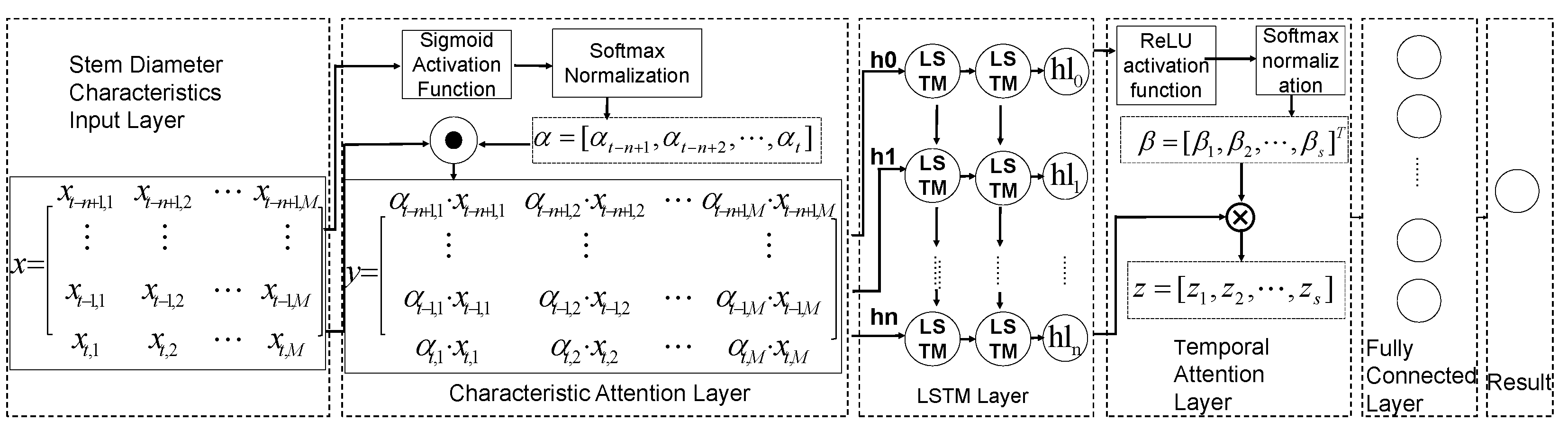
- We introduce the feature attention layer and the time-series attention layer in the LSTM framework to construct our stem diameter prediction model, and based on the SHAP (Shapley Additive Explanations) analysis algorithm [4] quantitatively analyzed the effects of various forestry factors on the growth and development of woolly poplar.
- We conduct comprehensive experiments using the control variable method and a module stacking strategy, validating our model’s significant advantages in effectiveness and stability.
2. Related Work
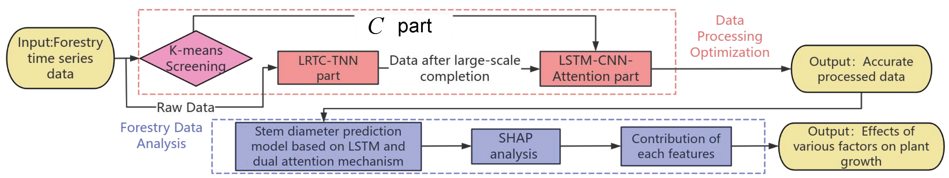
3. Method
3.1. Data Processing Optimization
3.1.1. Improved LRTC-TNN Model in
| Algorithm 1 Ip-LRTC-TNN |
| Require: , , Ensure: , Initialize for each attribute y in do if y is missing then replace y with end if end for while true do for each attribute k in do Updated by and end for Updated by and Updated by and Calculate from and if then break end if end while return |
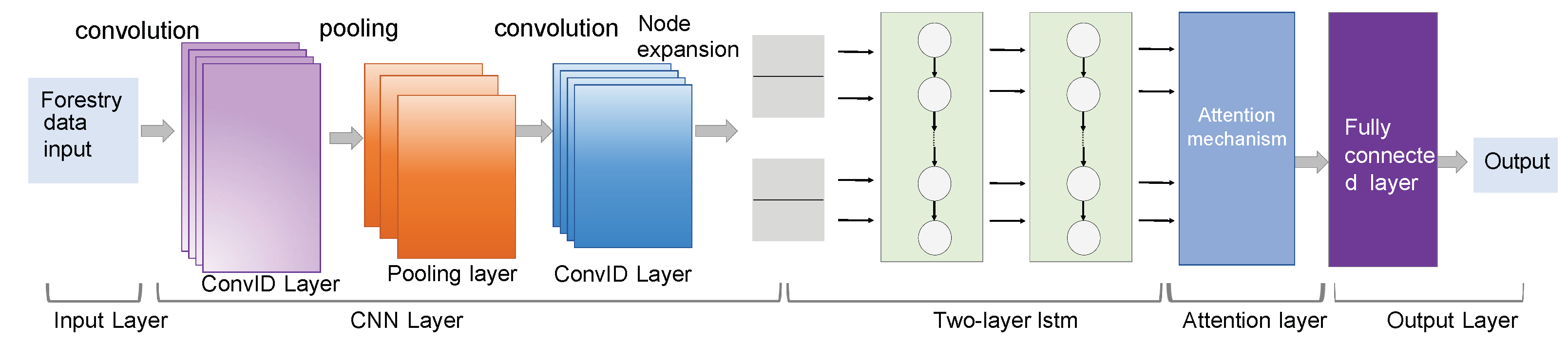
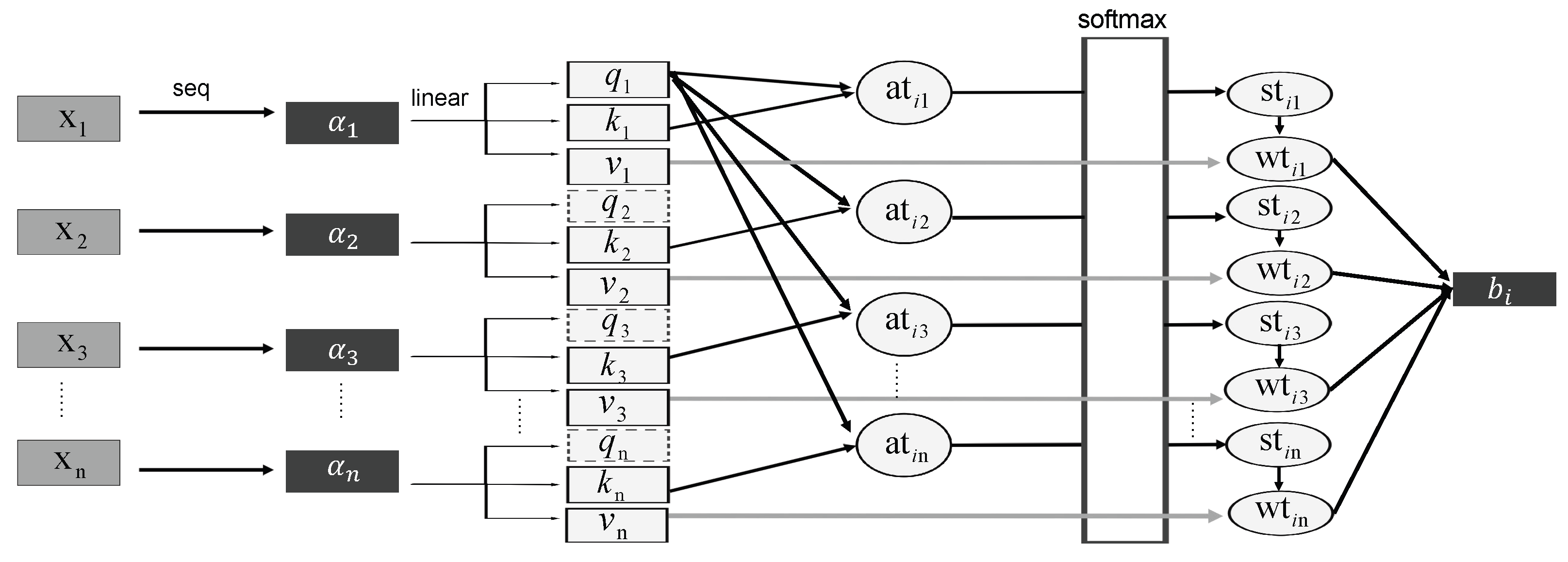
3.1.2. LSTM-CNN-Attention in
3.2. Forestry Data Analysis
4. Experiments
4.1. Dataset
4.2. Ablation Study
4.3. Comparative Analysis
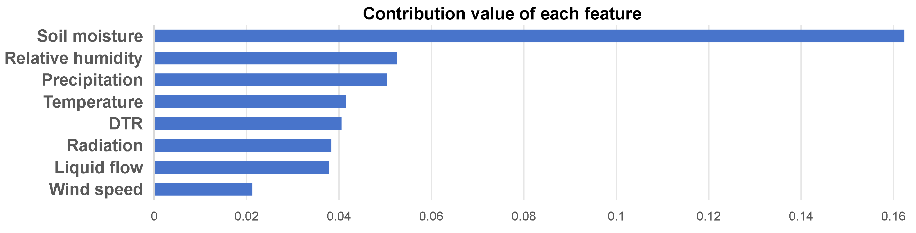
4.4. SHAP Interpretability
5. Conclusions
Author Contributions
Funding
Data Availability Statement
Conflicts of Interest
References
- Qiu, H.; Zhang, H.; Lei, K.; Zhang, H.; Hu, X. Forest digital twin: A new tool for forest management practices based on Spatio-Temporal Data, 3D simulation Engine, and intelligent interactive environment. Comput. Electron. Agric. 2023, 215, 108416. [Google Scholar] [CrossRef]
- Buonocore, L.; Yates, J.; Valentini, R. A Proposal for a Forest Digital Twin Framework and Its Perspectives. Forests 2022, 13, 498. [Google Scholar] [CrossRef]
- Li, W.; Yang, M.; Xi, B.; Huang, Q. Framework of Virtual Plantation Forest Modeling and Data Analysis for Digital Twin. Forests 2023, 14, 683. [Google Scholar] [CrossRef]
- Wang, X.; Ke, Z.; Liu, W.; Zhang, P.; Cui, S.A.; Zhao, N.; He, W. Compressive Strength Prediction of Basalt Fiber Reinforced Concrete Based on Interpretive Machine Learning Using SHAP Analysis. Iran. J. Sci. Technol. Trans. Civ. Eng. 2024, 49, 2461–2480. [Google Scholar] [CrossRef]
- Kabir, G.; Tesfamariam, S.; Hemsing, J.; Sadiq, R. Handling incomplete and missing data in water network database using imputation methods. Sustain. Resilient Infrastruct. 2020, 5, 365–377. [Google Scholar] [CrossRef]
- Yu, J.; Stettler, M.E.; Angeloudis, P.; Hu, S.; Chen, X.M. Urban network-wide traffic speed estimation with massive ride-sourcing GPS traces. Transp. Res. Part C Emerg. Technol. 2020, 112, 136–152. [Google Scholar] [CrossRef]
- Zhu, L.; Yang, L. Audio completion method based on tensor analysis. J. Phys. Conf. Ser. 2024, 2849, 012097. [Google Scholar] [CrossRef]
- Pan, J.; Zhong, S.; Yue, T.; Yin, Y.; Tang, Y. Multi-Task Foreground-Aware Network with Depth Completion for Enhanced RGB-D Fusion Object Detection Based on Transformer. Sensors 2024, 24, 2374. [Google Scholar] [CrossRef]
- Liao, T.; Wu, Z.; Chen, C.; Zheng, Z.; Zhang, X. Tensor completion via convolutional sparse coding with small samples-based training. Pattern Recognit. 2023, 141, 109624. [Google Scholar] [CrossRef]
- Cheng, F.; Peng, L.; Zhu, H.; Zhou, C.; Dai, Y.; Peng, T. A Defect Data Compensation Model for Infrared Thermal Imaging Based on Bi-LSTM with Attention Mechanism. JOM 2024, 76, 3028–3038. [Google Scholar] [CrossRef]
- Zhou, X.; Wang, H.; Xu, C.; Peng, L.; Xu, F.; Lian, L.; Deng, G.; Ji, S.; Hu, M.; Zhu, H.; et al. Application of kNN and SVM to predict the prognosis of advanced schistosomiasis. Parasitol. Res. 2022, 121, 2457–2460. [Google Scholar] [CrossRef] [PubMed]
- Saleti, S.; Panchumarthi, L.Y.; Kallam, Y.R.; Parchuri, L.; Jitte, S. Enhancing Forecasting Accuracy with a Moving Average-Integrated Hybrid ARIMA-LSTM Model. SN Comput. Sci. 2024, 5, 704. [Google Scholar] [CrossRef]
- Zhang, X.; Ren, H.; Liu, J.; Zhang, Y.; Cheng, W. A monthly temperature prediction based on the CEEMDAN–BO–BiLSTM coupled model. Sci. Rep. 2024, 14, 808. [Google Scholar] [CrossRef] [PubMed]
- Nikpour, P.; Shafiei, M.; Khatibi, V. Gelato: A new hybrid deep learning-based Informer model for multivariate air pollution prediction. Environ. Sci. Pollut. Res. 2024, 31, 29870–29885. [Google Scholar] [CrossRef]
- Tang, Y.; Yu, F.; Pedrycz, W.; Li, F.; Ouyang, C. Oriented to a multi-learning mode: Establishing trend-fuzzy-granule-based LSTM neural networks for time series forecasting. Appl. Soft Comput. 2024, 166, 112195. [Google Scholar] [CrossRef]
- Yang, W.; Zhang, Z.; Zhao, Y.; Gu, Y.; Huang, L.; Zhao, J. CABGSI: An efficient clustering algorithm based on structural information of graphs. J. Radiat. Res. Appl. Sci. 2024, 17, 101040. [Google Scholar] [CrossRef]
- Liu, J.; Musialski, P.; Wonka, P.; Ye, J. Tensor Completion for Estimating Missing Values in Visual Data. IEEE Trans. Pattern Anal. Mach. Intell. 2013, 35, 208–220. [Google Scholar] [CrossRef]
- Chen, X.; Yang, J.; Sun, L. A nonconvex low-rank tensor completion model for spatiotemporal traffic data imputation. Transp. Res. Part C 2020, 117, 102673. [Google Scholar] [CrossRef]
- Pandey, S. An Improved Analysis of TNN-Based Managed and Unverified Learning Approaches for Optimum Threshold Resolve. SN Comput. Sci. 2023, 4, 719. [Google Scholar] [CrossRef]
- Hien, L.T.K.; Papadimitriou, D. An inertial ADMM for a class of nonconvex composite optimization with nonlinear coupling constraints. J. Glob. Optim. 2024, 89, 927–948. [Google Scholar] [CrossRef]
- Jin, Z.F.; Fan, Y.; Shang, Y.; Ding, W. A dual symmetric Gauss-Seidel technique-based proximal ADMM for robust fused lasso estimation. Numer. Algorithms 2024, 98, 1337–1360. [Google Scholar] [CrossRef]
- Gholizadeh, M.; Saeedi, R.; Bagheri, A.; Paeezi, M. Machine learning-based prediction of effluent total suspended solids in a wastewater treatment plant using different feature selection approaches: A comparative study. Environ. Res. 2024, 246, 118146. [Google Scholar] [CrossRef] [PubMed]
- Linck, I.; Gómez, A.T.; Alaghband, G. SVG-CNN: A shallow CNN based on VGGNet applied to intra prediction partition block in HEVC. Multimed. Tools Appl. 2024, 83, 73983–74001. [Google Scholar] [CrossRef]
- Chagnon, J.; Hagenbuchner, M.; Tsoi, A.C.; Scarselli, F. On the effects of recursive convolutional layers in convolutional neural networks. Neurocomputing 2024, 591, 127767. [Google Scholar] [CrossRef]
- Wang, Y.; Zhang, Z.; Wang, Y.; You, L.; Wei, G. Modeling and structural optimization design of switched reluctance motor based on fusing attention mechanism and CNN-BiLSTM. Alex. Eng. J. 2023, 80, 229–240. [Google Scholar] [CrossRef]
- Zhang, S.; Xie, L. Advancing neural network calibration: The role of gradient decay in large-margin Softmax optimization. Neural Netw. 2024, 178, 106457. [Google Scholar] [CrossRef]
- Mao, Y.; Cheng, Y.; Shi, C. A Job Recommendation Method Based on Attention Layer Scoring Characteristics and Tensor Decomposition. Appl. Sci. 2023, 13, 9464. [Google Scholar] [CrossRef]
- Tang, Y.; Wang, Y.; Liu, C.; Yuan, X.; Wang, K.; Yang, C. Semi-supervised LSTM with historical feature fusion attention for temporal sequence dynamic modeling in industrial processes. Eng. Appl. Artif. Intell. 2023, 117, 105547. [Google Scholar] [CrossRef]
- Ramadevi, B.; Kasi, V.R.; Bingi, K. Fractional ordering of activation functions for neural networks: A case study on Texas wind turbine. Eng. Appl. Artif. Intell. 2024, 127, 107308. [Google Scholar] [CrossRef]
- Liu, H.; Li, L. Missing Data Imputation in GNSS Monitoring Time Series Using Temporal and Spatial Hankel Matrix Factorization. Remote Sens. 2022, 14, 1500. [Google Scholar] [CrossRef]
- Çelebi, M.; Öztürk, S.; Kaplan, K. An emotion recognition method based on EWT-3D–CNN–BiLSTM-GRU-AT model. Comput. Biol. Med. 2024, 169, 107954. [Google Scholar] [CrossRef] [PubMed]
- Xiaohui, H.; Yuan, J.; Jie, T. MAPredRNN: Multi-attention predictive RNN for traffic flow prediction by dynamic spatio-temporal data fusion. Appl. Intell. 2023, 53, 19372–19383. [Google Scholar]

| Method | DIA (um)↓ | SM (%)↓ | DTR (℃)↓ | LF (cm/s)↓ | TEMP (℃)↓ | RAD (W/m2)↓ | RH (%)↓ |
|---|---|---|---|---|---|---|---|
| +0Lr(+2C+A+2Ls) | 428.894504 | 1.317698 | 26.168093 | 0.015324 | 18.112322 | 431.690125 | 52.421295 |
| +0C(+Lr&+2L+A) | 359.140364 | 0.728776 | 17.662264 | 0.007894 | 6.112322 | 313.118481 | 27.512348 |
| +1C(+Lr&+2L+A) | 349.417584 | 0.451570 | 6.662314 | 0.004892 | 5.636185 | 264.615021 | 10.757118 |
| +3C(+Lr&+2L+A) | 354.854314 | 0.554539 | 12.530076 | 0.004969 | 6.077727 | 223.376731 | 11.173975 |
| +1L(+Lr&+2C+A) | 304.816727 | 0.602778 | 12.806879 | 0.005034 | 6.016144 | 231.242948 | 11.106624 |
| +3L(+Lr&+2C+A) | 302.975994 | 0.578611 | 3.980785 | 0.004998 | 5.974214 | 195.353134 | 10.067917 |
| +0A(+Lr&+2C+2L) | 502.550728 | 0.587159 | 21.142221 | 0.004866 | 6.045146 | 229.411539 | 14.266718 |
| (+Lr&+2C+A+2Ls) | 283.448347 | 0.365627 | 3.010184 | 0.004157 | 3.734599 | 205.375285 | 7.712643 |
| Method | DIA (um)↓ | SM (%)↓ | DTR (℃)↓ | LF (cm/s)↓ | TEMP (℃)↓ | RAD (W/m2)↓ | RH (%)↓ |
|---|---|---|---|---|---|---|---|
| +0Lr(+2C+A+2Ls) | 0.051337 | 0.771263 | 0.232126 | 0.002175 | 1.625194 | 3.375217 | 2.284953 |
| +0C(+Lr&+2L+A) | 0.051337 | 0.405597 | 0.197705 | 0.001496 | 0.449549 | 1.730600 | 0.729766 |
| +1C(+Lr&+2L+A) | 0.036108 | 0.021362 | 0.022602 | 0.000549 | 0.254312 | 0.842831 | 0.298929 |
| +3C(+Lr&+2L+A) | 0.038955 | 0.025341 | 0.023183 | 0.000678 | 0.278713 | 0.375205 | 0.285411 |
| +1L(+Lr&+2C+A) | 0.031656 | 0.025969 | 0.503459 | 0.000881 | 0.304089 | 0.421864 | 0.382649 |
| +3L(+Lr&+2C+A) | 0.032828 | 0.024768 | 0.022896 | 0.000648 | 0.270819 | 0.328273 | 0.285227 |
| +0A(+Lr&+2C+2L) | 0.047601 | 0.025075 | 0.024332 | 0.000817 | 0.296214 | 0.480572 | 0.409644 |
| (+Lr&+2C+A+2Ls) | 0.032449 | 0.017634 | 0.021184 | 0.000488 | 0.172258 | 0.354213 | 0.109663 |
| Method | BL | BL+F | BL+F+T | BL+F+T+2Ls | ALL (BL+F+T+Ls) |
|---|---|---|---|---|---|
| RMSE | 329.918288 | 208.372894 | 181.225549 | 172.334553 | 167.373654 |
| MASE | 0.019750 | 0.011900 | 0.010633 | 0.010056 | 0.009315 |
| Method | Ours | Lerp | ExpInterp | KNN | BTMF | BiLSTM-GRU | Transformers |
|---|---|---|---|---|---|---|---|
| DIA↓ | 283.448347 | 392.970190 | 392.968706 | 460.784986 | 344.282280 | 332.356781 | 335.611604 |
| SM ↓ | 0.365627 | 0.521159 | 0.521178 | 0.481712 | 0.451570 | 0.373310 | 0.420748 |
| DTR↓ | 3.010184 | 5.280655 | 5.717643 | 4.246914 | 9.532788 | 14.945592 | 8.217452 |
| LF↓ | 0.415709 | 0.510056 | 0.508245 | 0.7879 | 0.501073 | 0.406184 | 0.496458 |
| TEMP↓ | 3.734599 | 5.311704 | 5.307645 | 4.998622 | 5.636185 | 4.711132 | 9.337577 |
| RAD↓ | 205.375285 | 253.323734 | 254.571491 | 254.269126 | 233.928561 | 232.286006 | 242.198772 |
| RH↓ | 7.712643 | 7.803939 | 7.827227 | 9.337577 | 8.215242 | 8.114660 | 9.337577 |
| Method | Ours | Lerp | ExpInterp | KNN | BTMF | BiLSTM-GRU | Transformer |
|---|---|---|---|---|---|---|---|
| DIA↓ | 0.032449 | 0.042523 | 0.042525 | 0.049802 | 0.039562 | 0.036900 | 0.035601 |
| SM↓ | 0.017634 | 0.030785 | 0.030819 | 0.0270778 | 0.020389 | 0.017676 | 0.019759 |
| DTR↓ | 0.021184 | 0.026343 | 0.025908 | 0.040273 | 0.023344 | 0.020025 | 0.023918 |
| LF↓ | 0.000488 | 0.000504 | 0.000551 | 0.000492 | 0.000962 | 0.000783 | 0.000851 |
| TEMP↓ | 0.172258 | 0.209752 | 0.196836 | 0.221353 | 0.254312 | 0.2011534 | 0.229836 |
| RAD↓ | 0.304213 | 0.342371 | 0.341824 | 0.356714 | 0.323918 | 0.324967 | 0.343871 |
| RH↓ | 0.109663 | 0.109925 | 0.111515 | 0.110851 | 0.123816 | 0.121719 | 0.110742 |
| Method | Ours RMSE/MASE | RNN [32] RMSE/MASE | ARIMA-LSTM Hybrid [12] RMSE/MASE | BO-BiLSTM [13] RMSE/MASE | Informer [14] RMSE/MASE |
|---|---|---|---|---|---|
| DIA | 167.373654 | 397.583270 | 223.580558 | 191.700792 | 195.645380 |
| /0.009315 | /0.0185713 | /0.0122556 | /0.010274 | /0.010690 |
Disclaimer/Publisher’s Note: The statements, opinions and data contained in all publications are solely those of the individual author(s) and contributor(s) and not of MDPI and/or the editor(s). MDPI and/or the editor(s) disclaim responsibility for any injury to people or property resulting from any ideas, methods, instructions or products referred to in the content. |
© 2025 by the authors. Licensee MDPI, Basel, Switzerland. This article is an open access article distributed under the terms and conditions of the Creative Commons Attribution (CC BY) license (https://creativecommons.org/licenses/by/4.0/).
Share and Cite
Jiang, L.; Yang, M.; Xi, B.; Meng, W.; Duan, J. L2: Accurate Forestry Time-Series Completion and Growth Factor Inference. Forests 2025, 16, 895. https://doi.org/10.3390/f16060895
Jiang L, Yang M, Xi B, Meng W, Duan J. L2: Accurate Forestry Time-Series Completion and Growth Factor Inference. Forests. 2025; 16(6):895. https://doi.org/10.3390/f16060895
Chicago/Turabian StyleJiang, Linlu, Meng Yang, Benye Xi, Weiliang Meng, and Jie Duan. 2025. "L2: Accurate Forestry Time-Series Completion and Growth Factor Inference" Forests 16, no. 6: 895. https://doi.org/10.3390/f16060895
APA StyleJiang, L., Yang, M., Xi, B., Meng, W., & Duan, J. (2025). L2: Accurate Forestry Time-Series Completion and Growth Factor Inference. Forests, 16(6), 895. https://doi.org/10.3390/f16060895