Article

A Study on Airborne Hyperspectral Tree Species Classification Based on the Synergistic Integration of Machine Learning and Deep Learning

1
Beijing Yupont Electric Power Technology Co., Ltd., Beijing 100083, China
2
College of Forestry, Beijing Forestry University, Beijing 100083, China
*
Author to whom correspondence should be addressed.
Forests 2025, 16(6), 1032; https://doi.org/10.3390/f16061032
Submission received: 20 May 2025 / Revised: 15 June 2025 / Accepted: 16 June 2025 / Published: 19 June 2025
(This article belongs to the Section Forest Inventory, Modeling and Remote Sensing)

Abstract

Against the backdrop of global climate change and increasing ecological pressure, the refined monitoring of forest resources and accurate tree species identification have become essential tasks for sustainable forest management. Hyperspectral remote sensing, with its high spectral resolution, shows great promise in tree species classification. However, traditional methods face limitations in extracting joint spatial–spectral features, particularly in complex forest environments, due to the “curse of dimensionality” and the scarcity of labeled samples. To address these challenges, this study proposes a synergistic classification approach that combines the spatial feature extraction capabilities of deep learning with the generalization advantages of machine learning. Specifically, a 2D convolutional neural network (2DCNN) is integrated with a support vector machine (SVM) classifier to enhance classification accuracy and model robustness under limited sample conditions. Using UAV-based hyperspectral imagery collected from a typical plantation area in Fuzhou City, Jiangxi Province, and ground-truth data for labeling, a highly imbalanced sample split strategy (1:99) is adopted. The 2DCNN is further evaluated in conjunction with six classifiers—CatBoost, decision tree (DT), k-nearest neighbors (KNN), LightGBM, random forest (RF), and SVM—for comparison. The 2DCNN-SVM combination is identified as the optimal model. In the classification of Masson pine, Chinese fir, and eucalyptus, this method achieves an overall accuracy (OA) of 97.56%, average accuracy (AA) of 97.47%, and a Kappa coefficient of 0.9665, significantly outperforming traditional approaches. The results demonstrate that the 2DCNN-SVM model offers superior feature representation and generalization capabilities in high-dimensional, small-sample scenarios, markedly improving tree species classification accuracy in complex forest settings. This study validates the model’s potential for application in small-sample forest remote sensing and provides theoretical support and technical guidance for high-precision tree species identification and dynamic forest monitoring.

1. Introduction

With the intensification of global climate change and ecological challenges, dynamic monitoring and precise management of forest resources have become critical components of sustainable forestry development strategies [1,2]. Hyperspectral remote sensing, due to its ability to capture fine-grained spectral information of surface materials, has been widely applied in forest surveys and tree species classification tasks. Compared with traditional remote sensing imagery, hyperspectral images (HSIs) offer high spectral resolution and rich spectral detail, enabling fine discrimination of spectral differences among land cover types, and demonstrating great potential for distinguishing tree species in complex forest environments [3,4]. As a result, hyperspectral remote sensing is gradually becoming a key technological approach for accurate forest mapping and classification. However, the classification of hyperspectral forest imagery still faces two major challenges: (1) the high dimensionality of data and the difficulty of sample acquisition lead to the “curse of dimensionality”; and (2) the strong heterogeneity in tree species distribution and severe spectral mixing in complex forest regions hinder the ability of traditional algorithms to effectively extract joint spatial–spectral features, thereby limiting classification accuracy and model stability.
To address these challenges, researchers have extensively explored machine learning–based classification approaches [5]. Algorithms such as the support vector machine (SVM) [6,7], random forest (RF) [8], k-nearest neighbors (KNN) [9,10], and decision tree (DT) [11] algorithms have been widely used in hyperspectral image classification due to their theoretical maturity, high training efficiency, and strong adaptability to small sample sizes. These methods have shown superior generalization and robustness in handling high-dimensional features, limited sample availability, and blurred class boundaries, making them particularly suitable for the common “high-dimensional and small-sample” scenarios in hyperspectral data.
Building on these foundations, a growing number of studies have investigated feature extraction, fusion, and modeling techniques to fully exploit the rich spectral and spatial structural information in hyperspectral images [12]. For example, Liu et al. [13] proposed a classification method that integrates local binary pattern (LBP) texture features with image block reconstruction features and applied the KNN classifier, achieving overall accuracies of 99.06% and 99.73% on the Indian Pines and Pavia University datasets, respectively. This highlighted the critical role of spatial structure information in improving classification performance. Li et al. [14] systematically evaluated the combined effects of spectral preprocessing techniques (e.g., normalization and first-order derivatives) and classification algorithms (e.g., SVM and RF) using hyperspectral data of eight tree species from the Baguang Wetland Park in Shenzhen. Their results showed that first-order derivatives significantly enhanced inter-band variation trends, and when combined with RF, achieved an average classification accuracy of 76.65%, outperforming the SVM model (73.07%), thereby underscoring the importance of spectral preprocessing. Additionally, RF has been frequently applied in practical forest classification tasks due to its strengths in processing high-dimensional data, noise resistance, and model stability. For instance, Soleimannejad et al. [15] employed RF to effectively classify three major tree species in the Hyrcanian forests of Iran using multisource remote sensing data, including IRS-Pansharpened, Landsat-8, and Sentinel-2. They found that high-resolution IRS data and near-infrared bands were particularly effective in species differentiation. Moreover, machine learning methods have demonstrated good transferability in agroforestry ecotones and other land cover classification tasks. Tariq et al. [16] applied DT and RF to crop classification in Gujranwala, Pakistan, using fused Sentinel-2 and Landsat-8 data, achieving high-precision identification of crops such as tobacco, wheat, and barley, thus providing technical support for monitoring land cover in forest–agriculture transitional zones. Zhao et al. [17] combined stereo-microscopic hyperspectral imaging with a composite-kernel SVM model to achieve automated identification of timber species, offering a high-accuracy solution for forest product traceability and precise wood classification.
In recent years, with the development of deep learning, convolutional neural networks (CNNs) have demonstrated powerful automatic feature extraction capabilities for hyperspectral image classification, particularly in end-to-end modeling frameworks [18,19]. However, CNNs are highly dependent on large labeled datasets and are prone to overfitting under small-sample conditions. They also suffer from limitations in model interpretability and cross-regional generalization. To overcome these limitations, the synergistic integration of machine learning and deep learning has emerged as a new research trend. By combining the strong spatial feature extraction ability of two-dimensional CNNs (2DCNNs) with the robust performance of traditional classifiers such as SVM under small-sample settings, collaborative classification frameworks offer the potential for improved performance in limited-sample hyperspectral scenarios.
Based on the above analysis, this study proposes a collaborative 2DCNN-SVM method for tree species classification using airborne hyperspectral imagery. A typical plantation area in Fuzhou City, Jiangxi Province, is selected as the study area. Methodologically, a lightweight 2DCNN model is designed to extract spatial–spectral fusion features, and an SVM classifier is employed to replace the traditional MLP classifier, aiming to enhance model stability and classification accuracy under small-sample conditions. The main contributions of this study are as follows: (1) a collaborative 2DCNN-SVM hyperspectral classification framework suitable for small-sample scenarios is developed, effectively mitigating the deep learning model’s dependence on large-scale labeled data; (2) through parameter optimization and structural simplification, the model’s generalization and practical applicability are improved; and (3) by integrating high-resolution UAV-based hyperspectral imagery and ground survey data, the effectiveness of the proposed method in multi-species forest classification is validated, providing theoretical support and technical reference for forest resource monitoring and remote sensing-based mapping.

2. Overview of the Study Area and Data Acquisition

2.1. Overview of the Study Area

The study area is located in Fuzhou City, Jiangxi Province, China (116°07′ E, 27°87′ N), situated in the central-eastern part of the province. This region features a typical subtropical humid monsoon climate, characterized by warm and humid conditions with distinct seasonal variation. The annual average temperature is approximately 17.9 °C, the average annual precipitation is about 1900 mm, and the frost-free period lasts for around 248 days.
The topography is mainly composed of hills and low mountains, with elevations ranging from 100 to 400 m, and presents diverse geomorphological types. The geological structure is stable, and the predominant soil type is red soil, which provides favorable conditions for the growth of various tree and shrub species.
The study area is rich in forest resources, with a high vegetation coverage and a forest cover rate of 67.23%. Dominant tree species include Masson pine (Pinus massoniana), Chinese fir (Cunninghamia lanceolata), and eucalyptus (Eucalyptus spp.), which are distributed in a patchy and interlaced manner. These species form a typical southern China plantation ecosystem, offering both economic and ecological value. The spatial heterogeneity and mixed distribution of different tree species provide ideal conditions for spectral differentiation and classification modeling using hyperspectral imagery.
Overall, the region exhibits typical characteristics of subtropical forest ecosystems and complex terrain–vegetation structures. It is both representative and challenging, making it a suitable area for conducting hyperspectral remote sensing research on tree species classification and forest mapping. The geographical location of the study area is shown in Figure 1.

2.2. UAV-Based Hyperspectral Data Acquisition

The hyperspectral data used in this study were provided by Beijing Rigaa United Technology Co., Ltd. (Beijing, China), and acquired using the MicroCASI-1920 hyperspectral sensor (ITRES Research Limited, Calgary, AB, Canada) mounted on a UAV platform. The data were collected in July 2024, during the peak growing season of the vegetation, which is favorable for enhancing spectral differentiation among tree species.
The UAV operated in a fixed-wing configuration, flying at an altitude of 1000 m with a ground speed of 75 knots (approximately 139 km/h). The flight was designed with a forward overlap of 70% and a side overlap of 60% to ensure complete coverage of the study area and facilitate accurate image stitching. The acquired hyperspectral imagery achieved a spatial resolution of 0.5 m, providing both high spatial and spectral precision. The system was equipped with an Applanix APX-15 Inertial Navigation System (INS) integrated with an RTK-GNSS module, enabling centimeter-level positioning accuracy and offering a reliable foundation for subsequent classification analysis.
The MicroCASI-1920 sensor covers a spectral range of 400–1000 nm, comprising a total of 288 spectral bands with a spectral resolution better than 5 nm. It features a field of view (FOV) of 36.6°, enabling detailed capture of vegetation spectral characteristics. The sensor is integrated with an Applanix APX-15 Inertial Navigation System (INS) and supported by an RTK-GNSS system, which ensures centimeter-level positional and orientation accuracy.
During the flight missions, the UAV flew at a steady altitude of 1000 m and a speed of approximately 75 knots (about 139 km/h). The image acquisition was configured with a 70% forward overlap and a 60% side overlap, ensuring complete coverage of the study area. The resulting hyperspectral imagery has a spatial resolution of 0.5 m, providing high spatial and spectral fidelity that lays a solid foundation for subsequent land cover classification tasks.
After data acquisition, a series of preprocessing steps were conducted using dedicated software, including radiometric calibration, geometric correction, atmospheric correction, and band alignment. The final output consisted of orthorectified hyperspectral images with georeferencing information. The key technical specifications of the sensor used in this campaign are listed in Table 1.

2.3. Ground Survey Data Collection

To obtain accurate information on forest resources, validate the interpretation of remote sensing data, and provide essential support for tree species classification within the study area, a ground survey was conducted concurrently following the acquisition of hyperspectral data.
During the survey, a Leica TS60 total station (Leica Geosystems, Heerbrugg, Switzerland) and a South Surveying Lingrui S86 GNSS receiver (South Surveying & Mapping Instrument Co., Ltd., Guangzhou, China) were employed to precisely determine the boundaries of sample plots and the locations of various land cover features. In practice, the GNSS receiver operated in RTK mode to record the geographic coordinates of each plot, ensuring centimeter-level positioning accuracy. Meanwhile, the total station was used to survey plot boundaries, terrain features, and key land objects to further enhance spatial accuracy.
Sample plot selection followed principles of representativeness and balance. A total of nine 10 m × 10 m plots and eight 20 m × 20 m plots were surveyed, covering the main forest stand types and land cover categories in the study area. Within each plot, essential growth parameters of dominant tree species were recorded, including species name, tree height, diameter at breast height (DBH), crown width, and distribution density. For major species such as Pinus massoniana (Masson pine) and Cunninghamia lanceolata (Chinese fir), additional attributes such as estimated age, health status, and growth vigor were documented.
The survey results indicated that the dominant tree species in the study area include Pinus massoniana, Cunninghamia lanceolata, Eucalyptus spp., Camellia oleifera, and some young fir saplings, forming a multi-layered artificial forest structure. This ground survey effectively validated the tree species distribution observed in the hyperspectral data and provided reliable support for subsequent classification research.
As shown in Figure 2, to gain a deeper understanding of the spectral response characteristics of different tree species across hyperspectral bands, this study conducted a comparative analysis of the average reflectance curves of the major species. The results reveal that distinct spectral differences exist among species in specific wavelength ranges, particularly in the red-edge region and the near-infrared region. These differences provide a basis for subsequent feature extraction and classification modeling. Moreover, the analysis confirms the spectral separability among tree species, thereby strengthening the theoretical foundation for model development.

3. Research Methods

The UAV hyperspectral image classification method proposed in this study integrates machine learning with deep learning techniques and comprises the following five key stages:
(1)
Dataset Preparation:
The hyperspectral data were randomly partitioned into training and testing sets using a Python-based random sampling function. A strict 1% to 99% ratio was adopted to simulate scenarios with extremely limited labeled samples, thereby evaluating the model’s performance under small-sample conditions.
(2)
Construction of the Baseline 2D CNN Network:
The baseline network consists of two convolutional blocks, each containing n convolutional layers with a kernel size of 3 × 3. Following the convolutional blocks, a global average pooling layer and a fully connected layer are employed. This structure aims to enhance classification accuracy and generalization capability while reducing the risk of overfitting.
(3)
Baseline Model Optimization:
Parameter tuning is conducted on the baseline model to improve performance. The key hyperparameters optimized include spatial patch size, number of convolution kernels, and learning rate.
(4)
Development of the 2D CNN-SVM Classification Model:
To further improve classification performance, the multilayer perceptron (MLP) classifier in the baseline network is replaced with a support vector machine (SVM) classifier, which is better suited for limited sample scenarios and has demonstrated superior performance in high-dimensional data classification.
(5)
Accuracy Evaluation:
The classification performance is quantitatively assessed using overall accuracy (OA), average accuracy (AA), and the Kappa coefficient, ensuring a comprehensive evaluation of the model’s effectiveness.

3.1. Dataset Preparation

Based on field survey data, the study area was categorized into eight major land cover classes, including five forest vegetation types—Masson pine, Chinese fir, Chinese fir seedlings, eucalyptus, and camellia—as well as three non-forest types—bare land, water bodies, and roads. Ground-truth labels were manually annotated on the orthorectified hyperspectral imagery with reference to sample plot information. The spatial distribution of labeled ground samples is shown in Figure 3.
In the domain of hyperspectral image classification, particularly for forest resource mapping, the availability of labeled data is often severely constrained due to the high cost and difficulty of field data collection and annotation. Therefore, this study focuses on improving model performance under extremely limited labeled data conditions—an issue that has garnered increasing attention in recent literature. Previous studies have demonstrated that models trained on as little as 5% of available data can still achieve satisfactory results on several public hyperspectral datasets.
To simulate such small-sample scenarios, we adopted a 1:99 training-to-testing data split, with only 1% of the samples used for training and the remaining 99% for testing the model’s generalization capability. To ensure the robustness and reliability of the results, multiple independent experiments were conducted, a common practice in small-sample research. The detailed sample distribution is presented in Table 2.

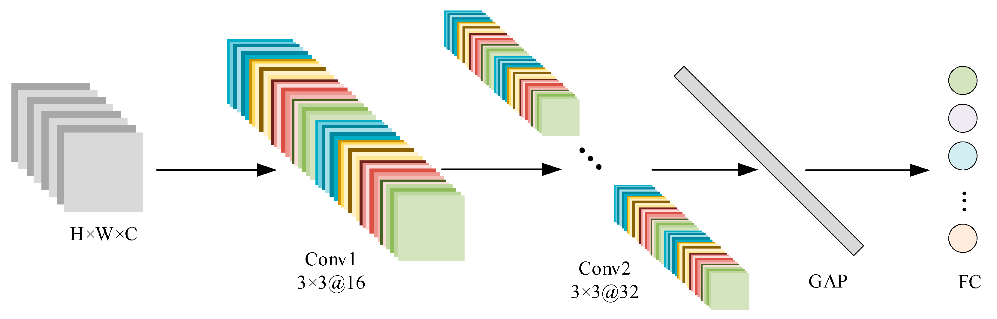
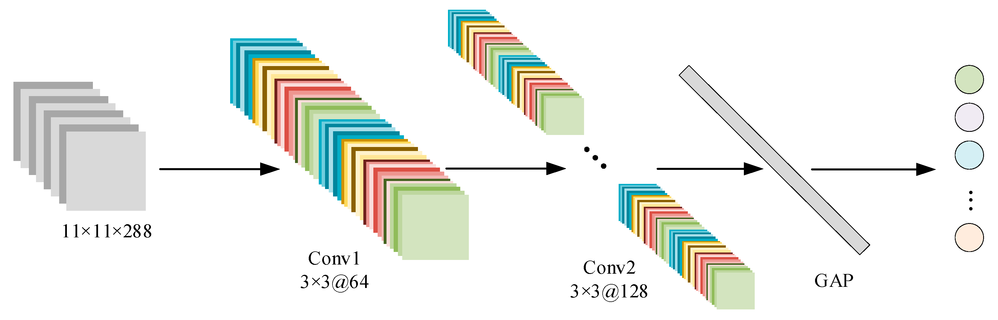
3.2. 2D Convolutional Neural Network (2DCNN) Classification Model

This study proposes a hyperspectral image classification method based on a two-dimensional convolutional neural network (2DCNN), which is designed to extract joint spatial–spectral features. The model architecture consists of convolutional modules, pooling and flattening layers, and fully connected layers. Spatial features are extracted using 2D convolution, and normalization and activation functions are employed to enhance feature representation and model stability.
(1)
Convolutional Module:
The convolutional block contains two 3 × 3 convolutional layers. The first layer uses 16 filters with a stride of 2 and padding of 1, followed by batch normalization and ReLU activation to enhance non-linear expressiveness and accelerate convergence. The second layer increases the number of channels to 32 to further improve feature extraction capability.
(2)
Pooling and Flattening Layer:
Instead of traditional pooling, global average pooling (GAP) is employed to compress the feature maps to a size of 1 × 1 × 32. This significantly reduces the number of parameters and enhances the extraction of global features. The output is then flattened into a one-dimensional vector for subsequent classification.
(3)
Fully Connected Layer:
A multi-layer perceptron (MLP) is used for classification, where the number of output nodes corresponds to the number of target classes.
The overall network is designed to enhance feature extraction while effectively suppressing overfitting. The architecture of the 2DCNN model is illustrated in Figure 4.

3.3. Optimization of the 2DCNN Model

The original 2DCNN model was optimized mainly from the following three aspects.

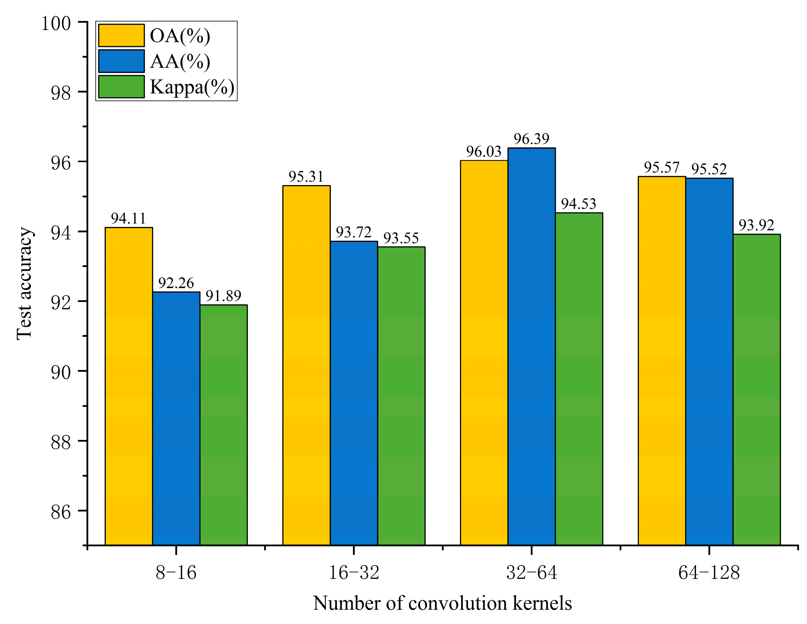
3.3.1. Optimization of the Number of Convolutional Kernels

In the 2DCNN model applied to hyperspectral image classification, the number of convolutional kernels directly affects the model’s feature extraction capability. An insufficient number of kernels limits the model’s ability to distinguish complex land cover types, while too many kernels introduce redundant features, increasing computational cost and potentially causing overfitting. In this study, comparative experiments were conducted to evaluate the number of kernels in the two convolutional layers, and the results are shown in Figure 5.
As the number of convolutional kernels increases, the overall accuracy (OA), average accuracy (AA), and Kappa coefficient first increase and then slightly decrease. This indicates that a reasonable number of kernels helps improve model performance, whereas an excessive number leads to performance degradation. When the number of kernels was set between 8 and 16, the OA, AA, and Kappa were 94.11%, 92.26%, and 0.9189 respectively, showing stable performance but not optimal classification accuracy. Increasing the kernels to the range of 16 to 32 improved all three metrics, demonstrating that this kernel count enables the extraction of richer features and enhances classification performance. Further increasing the kernels to 32 to 64 achieved the highest values for OA (96.03%), AA (96.39%), and Kappa (0.9453), indicating the best overall accuracy, class balance, and classification consistency at this configuration. However, when the number of kernels increased further to 64 to 128, all three indicators declined compared to the 32–64 range, with OA and AA decreasing to 95.57% and 95.52%, respectively. This drop is attributed to the redundancy introduced by excessive kernels, which increases model parameters and computational complexity, leading to overfitting on the training data and thereby reducing generalization ability.
In summary, a rational setting of the number of convolutional kernels plays a critical role in enhancing the performance of hyperspectral image classification models. An appropriate kernel count not only improves the model’s capability to express complex tree species features but also avoids the computational burden and overfitting caused by redundant parameters, achieving a good balance between classification accuracy and generalization.

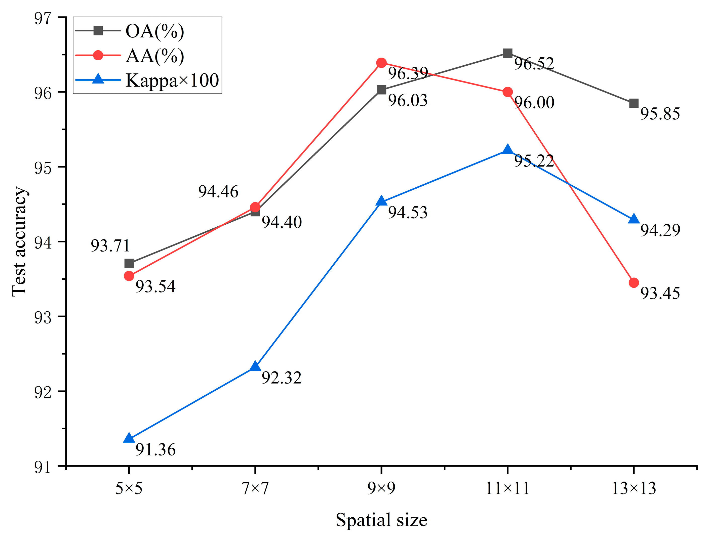
3.3.2. Optimization of Spatial Size

In the study of airborne hyperspectral image classification based on a two-dimensional convolutional neural network (2DCNN), reasonably setting the spatial size is crucial for preserving spatial feature information. An excessively large spatial size introduces noise and increases inference costs, while a size that is too small causes loss of critical information, limiting feature extraction capability. Therefore, experiments are necessary to determine the optimal parameter.
The results shown in Figure 6 indicate that the overall accuracy (OA), average accuracy (AA), and Kappa coefficient first increase and then decrease as the spatial size increases. Significant improvements are observed between sizes 5 × 5 and 11 × 11, with the best performance achieved at 11 × 11 (OA of 96.52%, AA of 96.00%, and Kappa of 0.9522). When the spatial size grows too large (13 × 13), redundant information and noise are introduced, resulting in decreased performance.
In forest remote sensing scenarios, tree species exhibit large variations in crown size and structural texture. A spatial size that is too small misses boundary information, while a size that is too large causes spectral–spatial confusion. Sizes of 5 × 5 and 7 × 7 focus on local features but lack contextual information, leading to lower accuracy. Sizes of 9 × 9 and 11 × 11 balance local and global contexts, thus improving classification performance. Although 13 × 13 covers a wider area, performance declines and computational complexity increases.
In summary, a reasonable spatial size helps balance effective feature acquisition and noise suppression. Optimizing spatial size not only improves the identification accuracy of tree species such as Masson pine, Chinese fir, and oil tea but also enhances the model’s adaptability to complex forest structures, providing high-precision support for forest resource surveys, forest stand map updates, and ecological monitoring.

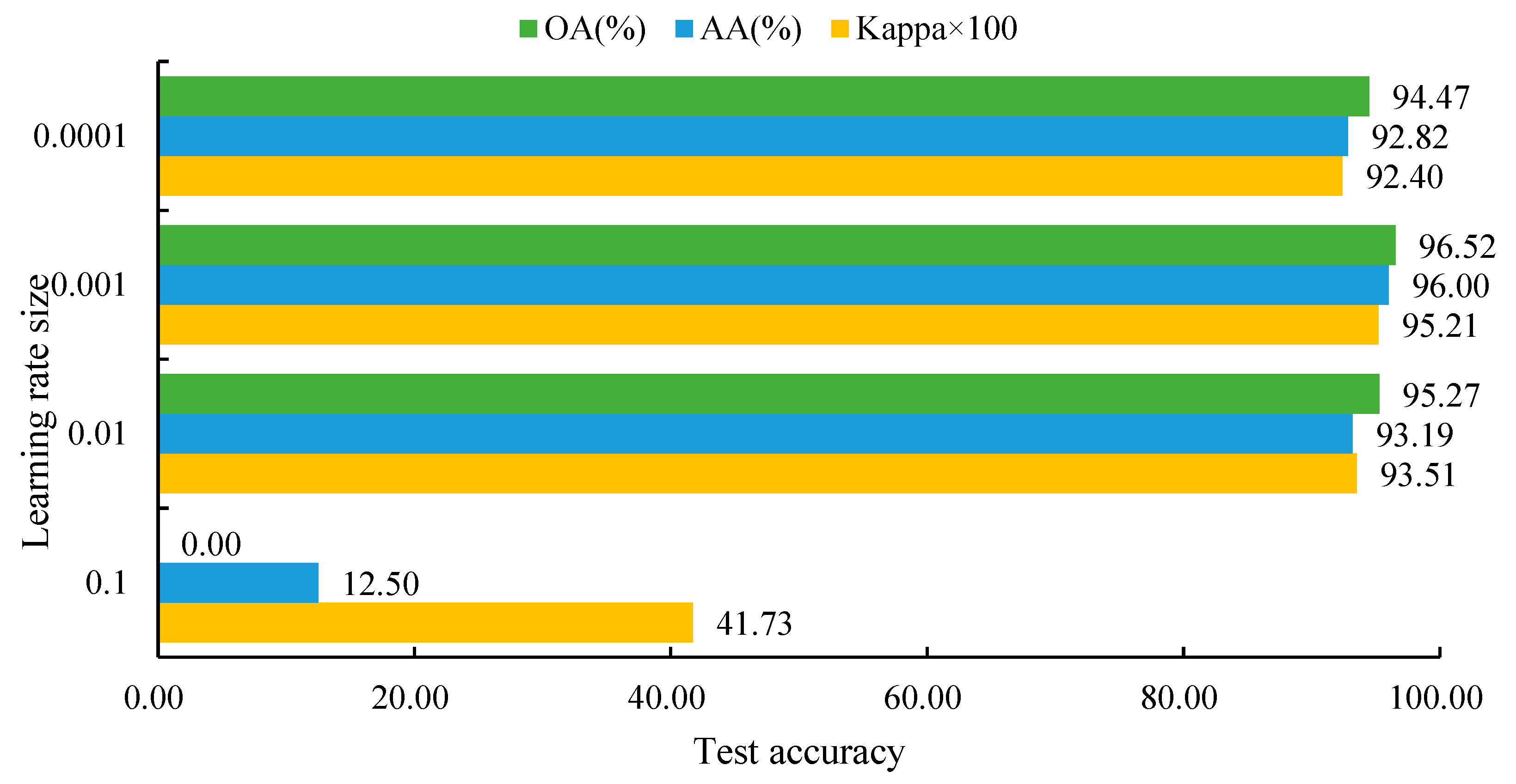
3.3.3. Learning Rate Optimization

The learning rate is a key hyperparameter influencing model performance, determining the step size of parameter updates, and directly affecting the model’s convergence speed and final accuracy. For high-dimensional hyperspectral data with strong correlations, a proper learning rate setting is especially critical for model stability and classification accuracy. An appropriate learning rate can accelerate convergence and improve performance; too large a learning rate causes model oscillation or failure to converge, while too small a learning rate results in slow training and difficulty in reaching the optimal solution.
To determine the optimal learning rate, a series of comparative experiments were conducted using values of 0.1, 0.01, 0.001, and 0.0001. As shown in Figure 7, a learning rate of 0.001 yielded the best classification performance, achieving the highest overall accuracy (OA), average accuracy (AA), and Kappa coefficient. This setting provided a good balance between convergence speed and model stability, and was therefore selected as the final learning rate for model training.
Figure 7 shows that different learning rates significantly impact the model’s classification results, exhibiting a “rise then fall” trend. When the learning rate is 0.1, the model fails to converge, with OA of 0.00%, AA of 12.50%, and Kappa of only 0.4173, indicating severe performance degradation. Reducing the learning rate to 0.01 leads to significant improvement, with OA reaching 95.27%, AA 93.19%, and Kappa 0.9351; the model tends toward convergence but is not yet optimal. Further reducing the learning rate to 0.001 achieves the best performance, with OA, AA, and Kappa of 96.52%, 96.00%, and 0.9521, respectively. At this rate, parameter updates are moderate, effectively suppressing gradient oscillations and allowing sufficient feature learning. Decreasing the learning rate further to 0.0001 causes performance to decline, with OA of 94.47%, AA of 92.82%, and Kappa of 0.9240, indicating that too small a learning rate limits training efficiency.
In summary, a learning rate of 0.001 yields the best model performance, achieving a good balance between convergence speed and accuracy, effectively enhancing the stability and generalization ability of hyperspectral tree species classification.

3.4. Construction of the 2DCNN-SVM Classification Model

To address challenges such as high dimensionality, limited sample size, and the limited capacity of traditional methods to model spatial features in hyperspectral image classification, this study adopts a two-dimensional convolutional neural network (2DCNN) as the primary feature extraction framework. Various classifiers including support vector machine (SVM), random forest (RF), decision tree (DT), K-nearest neighbors (KNN), CatBoost, and LightGBM are introduced for systematic comparison. After comprehensive evaluation of their performance in small-sample forest tree species recognition tasks, the SVM classifier, which demonstrated superior performance in terms of overall accuracy and robustness, was ultimately selected to enhance the classification capability and generalization of the model in complex forest scenarios.

3.4.1. Parameter Settings

The training parameters for each machine learning algorithm are configured as follows:
(1) K-Nearest Neighbors (KNN): The KNN algorithm determines the class of a sample by voting among its K nearest neighbors. In this experiment, the K value is set to 5, striking a balance between the model’s ability to capture local features and its sensitivity to local noise. A smaller K makes the model more sensitive to noise, while a larger K may ignore meaningful local patterns. Hence, K = 5 is chosen empirically for optimal performance.
(2) Support Vector Machine (SVM): In this study, the radial basis function (RBF) was selected as the kernel function for the SVM, as it effectively handles high-dimensional and non-linear classification problems. The kernel parameter gamma was set to “scale”, meaning it is automatically adjusted based on the number of features and the variance of the data, which helps improve model stability and adaptability across different scales. All parameters were tuned using a grid search approach, and the final combination (C = 100, gamma = “scale”) demonstrated strong classification performance and generalization ability on both the training and test sets.
(3) Random Forest (RF): For the RF algorithm, 500 decision trees are selected after comparative experiments to ensure strong performance while controlling computational cost. The random seed is set to 42 to ensure consistent model initialization across runs and reproducibility of the results.
(4) Decision Tree (DT): No explicit hyperparameter tuning is applied for the DT model, which uses default settings. The algorithm automatically selects optimal features and split points based on the input data. In many cases, the default parameters yield satisfactory performance while reducing the complexity of manual tuning.
(5) LightGBM: The parameters of LightGBM are configured to balance generalization and computational efficiency. The maximum tree depth is set to 6, the number of iterations to 500, and the learning rate to 0.03. These settings ensure a balance between accuracy and training efficiency.
(6) CatBoost: CatBoost’s parameters include the maximum number of iterations (default: 500), learning rate (default: 0.03), and maximum tree depth (set to 6). These parameters control model complexity, training time, and the contribution of each tree to the final prediction.

3.4.2. Selection of the Optimal Classifier Combining Machine Learning and Deep Learning

In UAV-based hyperspectral tree species classification tasks, the complexity and high dimensionality of the data make it difficult for a single model to fully extract discriminative information. To evaluate the effectiveness of combining 2DCNN with SVM, multiple machine learning classifiers were compared based on their utilization of features extracted by 2DCNN to identify the optimal combination. Table 3 presents the classification results of each method.
The 2DCNN–CatBoost combination performs stably, achieving an OA of 97.10%, AA of 96.39%, and Kappa of 0.9602. CatBoost demonstrates strong capabilities in feature interaction and noise resistance, performing well in classes such as young Cunninghamia lanceolata, bare soil, and lakes. However, its accuracy is lower for difficult-to-distinguish categories like eucalyptus and Camellia oleifera, indicating limitations in fine-grained classification.
In contrast, the DT classifier performs the weakest when combined with 2DCNN, with an OA of only 95.17%, as it tends to overfit on high-dimensional data and struggles to capture global features.
The KNN method shows high accuracy in certain classes, such as young C. lanceolata (99.47%) and roads (99.54%), but its overall OA is 96.88%. It suffers from the “curse of dimensionality,” where decision boundaries become blurred and computational complexity increases, limiting its applicability.
LightGBM achieves strong performance with an OA of 97.38% and a Kappa of 0.9640, especially for Pinus massoniana and C. lanceolata. However, it slightly underperforms compared to SVM and KNN in small-sample scenarios.
The RF model achieves an OA of 97.15% and a Kappa of 0.9608, demonstrating robust performance, particularly for classes like bare soil and lakes.
Among all combinations, 2DCNN-SVM delivers the best results across all metrics, with an OA of 97.56%, AA of 97.47%, and Kappa of 0.9665. SVM is capable of constructing an optimal hyperplane in high-dimensional space and possesses strong generalization capabilities. It is especially suitable for small-sample scenarios and fully leverages the features extracted by 2DCNN.
In conclusion, 2DCNN-SVM performs the best in hyperspectral tree species classification, while LightGBM and RF offer good stability and efficiency. KNN and DT exhibit weaker adaptability and are less suited for complex, high-dimensional classification tasks.

3.4.3. Construction of the 2DCNN-SVM Classification Model

Support vector machines (SVMs) demonstrate excellent classification capabilities, particularly in handling nonlinearly separable problems, by constructing an optimal hyperplane and maximizing the margin between classes. This results in strong generalization ability and effectively mitigates the overfitting problem often encountered in 2D convolutional neural networks (2DCNNs), thereby enhancing the model’s adaptability and classification accuracy on unseen data. In the context of forest remote sensing, where spectral differences between tree species are subtle and boundaries are often ambiguous, conventional neural networks struggle to achieve accurate classification. By leveraging support vectors to construct clear decision boundaries in the feature space, SVMs can effectively distinguish spectrally similar species such as Masson pine, camellia, and Chinese fir, improving the model’s discriminative power and stability.
To address the limitations of 2DCNNs in complex data scenarios—specifically, unclear class boundaries and limited accuracy—this study replaces the traditional multi-layer perceptron (MLP) classifier with an SVM, forming a 2DCNN-SVM hybrid model. The proposed model features a compact and efficient architecture, consisting of two convolutional layers, a global average pooling layer, and an SVM classifier (as illustrated in Figure 8; detailed parameters are listed in Table 4).
The first convolutional layer uses 3 × 3 kernels with 64 channels, a stride of 2, and padding of 1. It is followed by a batch normalization layer and a ReLU activation function, which jointly accelerate convergence and enhance nonlinear feature representation. The second convolutional layer maintains the same kernel size and stride while increasing the number of channels to 128, further strengthening feature extraction capabilities. Subsequently, a global average pooling layer is applied to significantly reduce the number of parameters and computational complexity while extracting more generalizable global features.
Finally, the deep features extracted by the convolutional layers are input into the SVM classifier for final prediction. SVM is particularly effective at handling high-dimensional feature spaces, making it well suited for the complex class differentiation required in hyperspectral image classification. By integrating the feature learning strength of CNNs with the robust decision-making ability of SVMs, the 2DCNN-SVM model achieves improved classification accuracy and enhanced overall stability, offering a reliable and efficient solution for hyperspectral tree species recognition.

3.5. Evaluation Metrics

In this study, overall accuracy (OA), average accuracy (AA), and the Kappa coefficient are employed to assess the classification performance [20]. By utilizing these evaluation metrics along with repeated cross-validation, the study aims to comprehensively and objectively evaluate the effectiveness of different classification algorithms in tree species classification using hyperspectral imagery.
OA is the most intuitive metric for measuring the performance of a classification model, representing the percentage of correctly classified samples out of the total number of samples. It is calculated as follows:
O A = T P + T N T P + T N + F P + F N
Here, TP, TN, FP, and FN denote true positives, true negatives, false positives, and false negatives, respectively.
AA refers to the average accuracy across all classes, reflecting the model’s classification performance for each individual class. It is calculated as follows:
A A = 1 N i = 1 N T P i T P i + F N i
where N is the number of categories and TPi and TPi + FNi denote the actual positive and total positive samples for category i, respectively.
The Kappa coefficient measures the degree of agreement between the classification results and the actual samples, reducing the bias that may arise from relying solely on accuracy. The formula for Kappa is as follows:
K a p p a = P o P e 1 P e
where Po is the overall accuracy and Pe is the expected accuracy due to random chance.

3.6. Environmental Settings

This study was conducted in a Python 3.8 environment, utilizing PyTorch 2.3 as the deep learning framework, and executed on a Windows 11 operating system. The model is based on a 2D convolutional neural network (2DCNN), with an initial learning rate set to 0.001. The Adam optimizer was employed using default parameters (β1 = 0.9, β2 = 0.999, eps = 1 × 10⁻⁸). The cross-entropy loss function was used for optimization. The batch size was set to 128, and the number of training epochs was 20. To reduce the randomness of the experiments, the final results were obtained by averaging the outcomes of five independent runs, and the accuracy reported for each experiment is the mean value.

4. Classification Results and Analysis

4.1. Classification Results of the 2DCNN Model

To comprehensively evaluate the performance of the 2DCNN model in tree species classification, Table 5 presents the confusion matrix based on our self-constructed UAV hyperspectral dataset from Jiangxi. The matrix displays the number of actual and predicted samples for each class, along with the corresponding producer’s accuracy (PA) and user’s accuracy (UA). By analyzing the confusion matrix, the model’s classification accuracy and confusion tendencies across categories can be thoroughly assessed.
From an overall perspective, the 2DCNN model demonstrates strong classification capabilities for most major tree species. For instance, 120,830 samples of Masson pine and 181,133 samples of Chinese fir were correctly classified, with producer’s accuracies of 94.84% and 95.28%, respectively. Their user’s accuracies both exceeded 94%, indicating the model’s robust discriminative power for these frequent categories. However, there is notable confusion between Masson pine and Chinese fir: 6367 Masson pine samples were misclassified as Chinese fir, while 6627 Chinese fir samples were misclassified as Masson pine. This suggests substantial spectral similarity between the two species, which poses a significant challenge for accurate discrimination and remains a major bottleneck for further performance improvement.
A closer look at other classes reveals that Chinese fir saplings, bare soil, and water bodies exhibit particularly high classification accuracies. The producer’s and user’s accuracies for Chinese fir saplings reached 99.05% and 97.96%, respectively. Bare soil achieved producer’s and user’s accuracies of 99.86% and 96.81%, while water bodies recorded 99.38% and 99.97%, respectively. These results suggest that such classes have more distinctive and stable spectral signatures, allowing the model to extract discriminative features more effectively and achieve more reliable classification performance.
In contrast, the classification performance for Camellia oleifera (oil tea) is relatively poor, with both producer’s and user’s accuracies at 74.53%, the lowest among all categories. The majority of misclassifications were as Chinese fir, with 1667 oil tea samples incorrectly labeled as such. Additional misclassifications occurred with Chinese fir saplings and eucalyptus. This outcome further confirms the strong overlap of spectral features between oil tea and other species, which limits the model’s discriminative ability for this class. Moreover, the relatively smaller number of oil tea samples compared to dominant species may have hindered sufficient feature learning, aggravating the misclassification issue.
In summary, the 2DCNN model achieves high classification accuracy for categories with distinct spectral characteristics, indicating its strong capability in feature extraction and pattern recognition. However, for tree species such as oil tea, which exhibit high spectral similarity to other categories, the model’s classification performance remains suboptimal. Future research may focus on incorporating more heterogeneous information (e.g., spatial texture, structural features), improving sample balance strategies, or integrating deeper discriminative mechanisms to enhance the model’s ability to distinguish confusing classes and improve its generalizability and applicability in complex forest environments.

4.2. Comparative Analysis Between the 2DCNN-SVM Model and Mainstream Classification Models

To comprehensively evaluate the classification performance of the 2DCNN-SVM model, it was compared with five mainstream classification models: 1D-CNN, 2DCNN+PCA, RNN, 3D-CNN, MLP, RoF [21], and ABTSVM [22] The comparison was conducted from two perspectives: classification accuracy and visual analysis.

4.2.1. Comparative Experiment Analysis

As shown in Table 6, the 2DCNN-SVM model achieved the highest overall accuracy (OA) of 97.56%, average accuracy (AA) of 97.47%, and Kappa coefficient of 0.9665 in hyperspectral tree species classification, indicating its superior overall performance and consistency. For the classification of Camellia oleifera, the 2DCNN-SVM model achieved an accuracy of 92.36%, significantly outperforming 1DCNN and MLP (64.15%), as well as 2DCNN+PCA (56.61%), demonstrating its advantage in handling complex and easily confused categories. For eucalyptus, it achieved 94.48%, slightly lower than 3D-CNN (95.24%) but superior to the remaining models. The combination of deep features extracted by 2DCNN and the optimal hyperplane construction capability of SVM in high-dimensional feature spaces effectively enhanced classification performance.
The RoF model exhibited moderate performance across most categories, but its accuracy dropped significantly in complex classes such as Camellia oleifera (50.57%) and eucalyptus (78.75%), much lower than that of 2DCNN-SVM. This indicates that RoF struggles to distinguish between spectrally similar and boundary-blurred classes. However, for categories with distinct spectral signatures such as bare land and water bodies, RoF performed well, achieving 99.53% and 99.91% accuracy respectively, reflecting its robustness in clearly separable classes.
The ABTSVM model demonstrated strong competitiveness in most forest categories. For instance, its classification accuracy for Camellia oleifera reached 92.96%, slightly higher than that of 2DCNN-SVM (92.36%). For eucalyptus, it achieved 91.66%, which, although slightly lower than 3D-CNN and 2DCNN-SVM, was significantly better than RoF and traditional methods like MLP. By integrating adaptive boundary tuning and multi-class SVM strategies, ABTSVM enhanced its capability to capture complex decision boundaries, showing good performance in classifying spectrally similar tree species. However, its performance in dominant classes such as Masson pine and Chinese fir remained slightly inferior to 2DCNN-SVM, suggesting potential limitations in spatial feature extraction.
In contrast, the 2DCNN+PCA and 2DCNN+1DCNN models exhibited relatively poor performance, with OA values of 87.99% and 90.83%, AA values of 87.90% and 92.60%, and Kappa coefficients of 0.8345 and 0.8737, respectively. The decline in performance was mainly due to the loss of critical information during PCA-based dimensionality reduction. Additionally, the 1DCNN and MLP models achieved only 64.15% accuracy for Camellia oleifera, as they relied solely on spectral features and neglected spatial information, limiting their applicability to complex categories.
In summary, the 2DCNN-SVM model effectively combines the automatic feature extraction capability of CNN with the classification strength of SVM, resulting in higher accuracy and robustness in hyperspectral tree species classification. This collaborative approach integrates the advantages of deep learning and traditional machine learning, significantly improving the model’s generalization ability and classification performance.
The confusion matrix in Figure 9 visually illustrates the classification performance of different models on UAV-based hyperspectral imagery, highlighting the per-class accuracies and potential misclassification patterns.

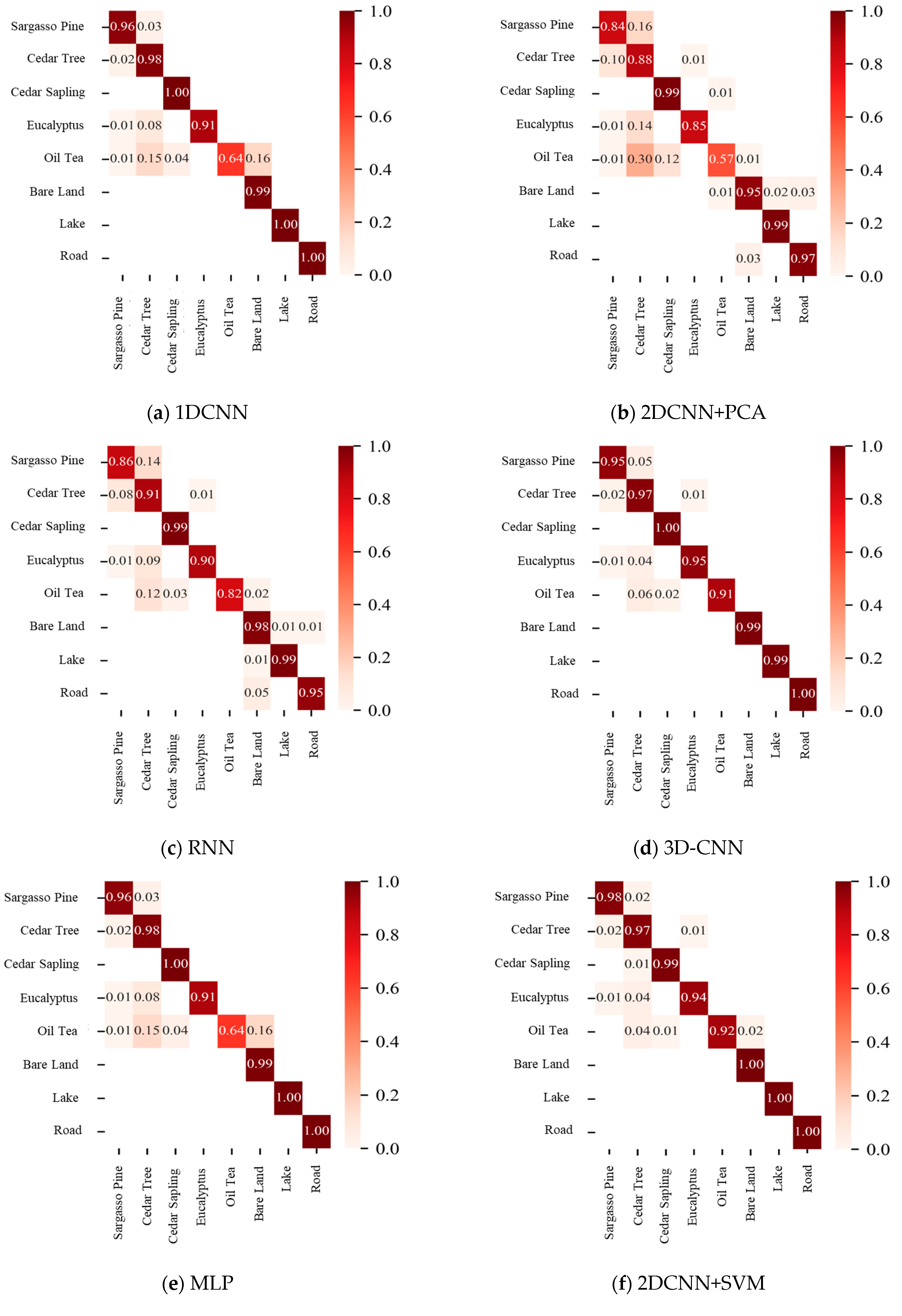
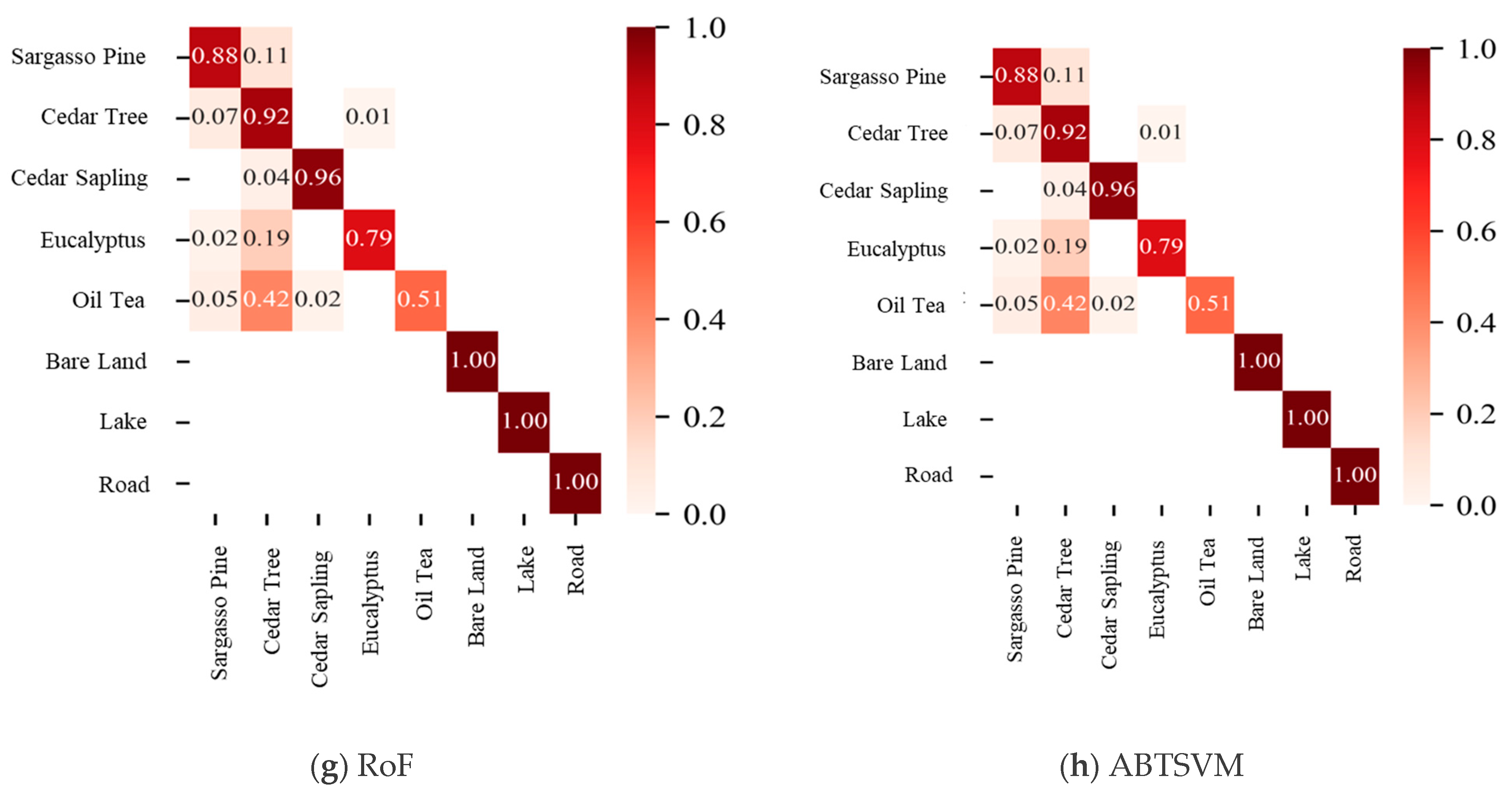
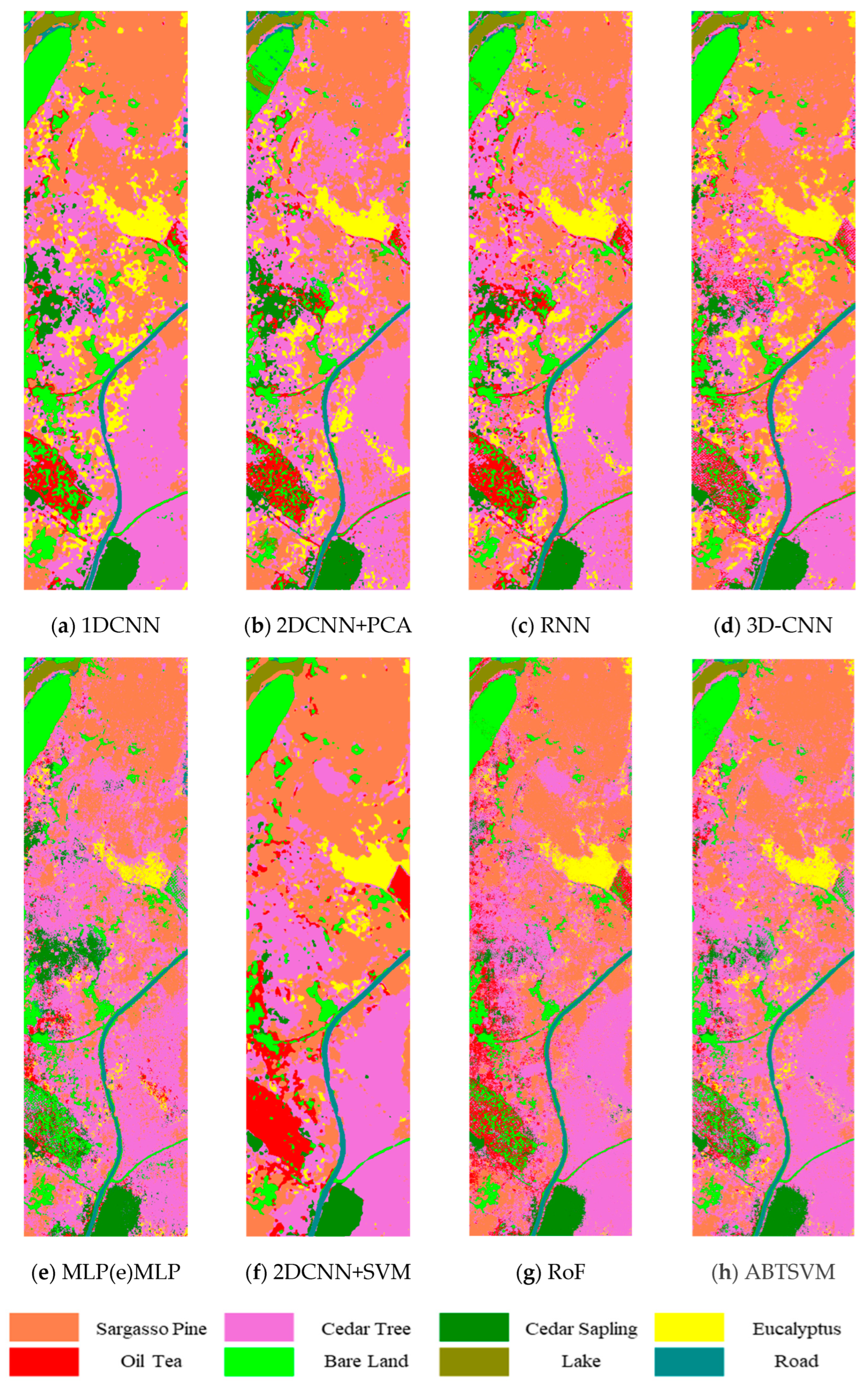
4.2.2. Visualization Analysis of Classification Results from Different Models

In this study, we visualized the classification results of various methods for hyperspectral imagery; Figure 10 presents the resulting classification maps. 1DCNN (Figure 10a) exhibits blurred class boundaries, as it relies solely on spectral information and neglects spatial context, resulting in misclassifications for spectrally similar adjacent classes such as Masson pine and Chinese fir. 2DCNN+PCA (Figure 10b) and RNN (Figure 10c) produce clearer boundaries, yet still confuse eucalyptus and Masson pine, likely due to similar canopy structures in dense or young stands. 3D-CNN (Figure 10d) performs well in complex scenes but shows blurred regions in small-sample scenarios, reflecting its sensitivity to sample size and class imbalance. MLP (Figure 10e) achieves clear classification for Masson pine and roads but still misclassifies other conifers.
While RoF (Figure 10g) performs well for distinct non-forest classes such as bare land and water bodies, it struggles in forested areas—particularly between Camellia oleifera and eucalyptus—due to insufficient spatial contextual modeling in its handling of high-dimensional hyperspectral data. ABTSVM (Figure 10h) achieves reasonable performance for certain species (e.g., Chinese fir), but misclassifications persist between Masson pine and eucalyptus. Although ABTSVM attains high accuracy for Camellia oleifera, its boundary delineation remains inferior to that of 2DCNN-SVM, indicating limited discrimination in complex mixed forests.
By contrast, the 2DCNN-SVM method (Figure 10f) demonstrates the clearest class boundaries and best overall classification performance. The 2DCNN component effectively captures spatial patterns such as canopy shape, row planting structure, and gap distribution, whereas the SVM classifier leverages these features for precise decision-making. This synergy addresses misclassification at class boundaries and delivers high accuracy and stability. The collaborative use of CNN for feature extraction and SVM for classification makes 2DCNN-SVM the most effective method for hyperspectral forest scene classification. It holds strong potential for applications in automating forest resource monitoring, species-level mapping, and detection of pest and disease areas in diverse subtropical forests.

5. Conclusions

This study demonstrates that the proposed 2DCNN-SVM model effectively improves the accuracy and robustness of tree species classification using UAV-based hyperspectral imagery, particularly under small-sample conditions. A two-dimensional convolutional neural network (2DCNN) was employed to automatically extract multi-level spatial–spectral features from hyperspectral images, enabling efficient modeling of complex nonlinear relationships in the data. Key hyperparameters, including the number of convolution kernels, spatial patch size, and learning rate, were carefully optimized to enhance feature representation and model stability.
To overcome the overfitting tendency of multilayer perceptrons (MLPs) under limited training samples, a support vector machine (SVM) was introduced to replace MLP, forming an efficient 2DCNN-SVM classification model. The SVM’s ability to construct optimal separating hyperplanes in high-dimensional spaces significantly improved the model’s generalization capability.
Experiments were conducted using a self-built hyperspectral dataset from typical plantation areas in Jiangxi Province. Evaluation metrics included the confusion matrix, overall accuracy (OA), average accuracy (AA), and Kappa coefficient. The results demonstrated that the 2DCNN-SVM model achieved outstanding performance, particularly in distinguishing confusing species such as Camellia oleifera and eucalyptus, with an OA of 97.56%, AA of 97.47%, and a Kappa coefficient of 0.9665. The model significantly outperformed baseline methods including 1DCNN, 2DCNN+PCA, 3D-CNN, and MLP. Parameter optimization experiments further validated the robustness and generalization ability of the proposed model in both feature extraction and classification decision-making.
This study achieved high-accuracy recognition of typical southern plantation species under limited sample conditions, laying a technical foundation for large-scale and cross-regional forest remote sensing classification and dynamic monitoring. The proposed 2DCNN-SVM collaborative modeling strategy demonstrates strong generalizability and is potentially applicable to more complex forest classification tasks, such as those in agroforestry ecotones.
Future work can be extended in several directions: (1) integrating spectral dimensionality reduction and data augmentation techniques to improve robustness in small-sample training; (2) incorporating multi-source remote sensing data (e.g., LiDAR, SAR) for multimodal classification; (3) adopting attention mechanisms or transfer learning frameworks to enhance spatial generalization; and (4) constructing larger and more representative hyperspectral forest sample databases to facilitate practical deployment of the proposed model in forest resource monitoring.

Author Contributions

Conceptualization, D.Y.; methodology, D.Y.; software, D.Y.; validation, D.Y. and J.S.; formal analysis, D.Y. and C.H.; investigation, D.Y.; resources, D.Y.; data curation, D.Y.; writing—original draft preparation, D.Y.; writing—review and editing, D.Y.; visualization, F.Y.; supervision, D.Y., J.S., C.H., F.Y., Y.H. and R.W.; project administration, D.Y. All authors have read and agreed to the published version of the manuscript.

Funding

This study was supported by An Impact Assessment and Biodiversity Conservation Study on Habitat Quality of Typical Wildlife Taxa under the “Liangjiang-Sihe” Afforestation and Greening Project (XZ202501YD0016) and the National Natural Science Foundation of China, 41971376.

Data Availability Statement

Data are contained within the article.

Conflicts of Interest

Authors Dabing Yang, Jinxiu Song, Chaohua Huang, Fengxin Yang and Yiming Han were employed by the company Beijing Yupont Electric Power Technology Co., Ltd. The remaining authors declare that the research was conducted in the absence of any commercial or financial relationships that could be construed as a potential conflict of interest.

References

  1. Kampouri, M.; Kolokoussis, P.; Argialas, D.; Karathanassi, V. Mapping of Forest Tree Distribution and Estimation of Forest Biodiversity using Sentinel-2 Imagery in the University Research Forest Taxiarchis in Chalkidiki, Greece. Geocarto Int. 2018, 34, 1273–1285. [Google Scholar] [CrossRef]
  2. Dosovitskiy, A.; Beyer, L.; Kolesnikov, A.; Weissenborn, D.; Zhai, X.; Unterthiner, T.; Dehghani, M.; Minderer, M.; Heigold, G.; Gelly, S.; et al. An Image is Worth 16x16 Words: Transformers for Image Recognition at Scale. arXiv 2020, arXiv:2010.11929. [Google Scholar]
  3. Fassnacht, F.E.; Latifi, H.; Stereńczak, K.; Modzelewska, A.; Lefsky, M.; Waser, L.T.; Straub, C.; Ghosh, A. Review of studies on tree species classification from remotely sensed data. Remote Sens. Environ. 2016, 186, 64–87. [Google Scholar] [CrossRef]
  4. Markov, N.G.; Machuca, C.R. Deep learning models and methods for solving the problems of remote monitoring of forest resources. Bull. Tomsk. Polytech. Univ. Geo Assets Eng. 2024, 35. [Google Scholar]
  5. Sothe, C.; De, A.C.M.; Schimalski, M.B.; La, R.L.E.C.; Castro, J.D.B.; Feitosa, R.Q.; Dalponte, M.; Lima, C.L.; Liesenberg, V.; Miyoshi, G.T.; et al. Comparative performance of convolutional neural network, weighted and conventional support vector machine and random forest for classifying tree species using hyperspectral and photogrammetric data. GISci. Remote Sens. 2020, 57, 369–394. [Google Scholar] [CrossRef]
  6. Chen, Y.; Liu, Z.; Chen, Z. AMS: A hyperspectral image classification method based on SVM and multi-modal attention network. Knowl.-Based Syst. 2025, 314, 113236. [Google Scholar] [CrossRef]
  7. Wang, H.; Li, G.; Wang, Z. Fast SVM classifier for large-scale classification problems. Inf. Sci. 2023, 642, 119136. [Google Scholar] [CrossRef]
  8. Pan, S.; Guan, H.; Yu, Y.; Li, J.; Peng, D. A Comparative Land-Cover Classification Feature Study of Learning Algorithms: DBM, PCA, and RF Using Multispectral LiDAR Data. IEEE J.-Stars 2019, 12, 1314–1326. [Google Scholar] [CrossRef]
  9. Bhavatarini, N.; Akash, B.N.; Akshay, H.M. Object Detection and Classification of Hyperspectral Images Using K-NN. In Proceedings of the 2023 Second International Conference on Electrical, Electronics, Information and Communication Technologies, Trichirappalli, India, 5–7 April 2023; pp. 1–7. [Google Scholar]
  10. Pal, M.; Charan, T.B.; Poriya, A. K-nearest neighbour-based feature selection using hyperspectral data. Remote Sens. Lett. 2021, 12, 132–141. [Google Scholar] [CrossRef]
  11. Yang, H.; Wang, J.; Su, B. Fast processing method of high resolution remote sensing image based on decision tree classification. Aerosp. Electron. 2020, 1, 1–11. [Google Scholar]
  12. Abidi, S.; Sellami, A. Attention-driven multi-feature fusion for hyperspectral image classification via multi-criteria optimization and multi-view convolutional neural networks. Eng. Appl. Artif. Intel. 2024, 138, 109434. [Google Scholar] [CrossRef]
  13. Liu, J.M.; Zheng, C.; Zhang, L.M.; Zou, Z.H. Hyperspectral Image Classification Based on Image Reconstruction and Feature Fusion. Laser Infrared 2021, 48, 203–212. [Google Scholar]
  14. Li, D.; Huang, Y.H.; Sun, Z.Y.; Zhang, W.Q.; Gan, X.H.; Wang, Z.L.; Sun, H.B.; Yang, L. Hyperspectral Classification of Tree Species in Bagang Wetland Park, Shenzhen, Based on Machine Learning. Infrared 2019, 40, 47–52. [Google Scholar]
  15. Soleimannejad, L.; Ullah, S.; Abedi, R.; Dees, M.; Koch, B. Evaluating the potential of sentinel-2, landsat-8, and irs satellite images in tree species classification of Hyrcanian Forest of Iran using random forest. J. Sustain. For. 2019, 38, 615–628. [Google Scholar] [CrossRef]
  16. Tariq, A.; Yan, J.; Gagnon, A.S.; Riaz Khan, M.; Mumtaz, F. Mapping of cropland, cropping patterns and crop types by combining optical remote sensing images with decision tree classifier and random forest. Geo-Spat. Inf. Sci. 2023, 26, 302–320. [Google Scholar] [CrossRef]
  17. Zhao, P.; Tang, Y.H.; Li, Z.Y. Tree Species Classification of Hyperspectral Microscopic Imaging Wood Based on Support Vector Machine with Composite Kernel Function. Spectrosc. Spectr. Anal. 2019, 39, 3776–3782. [Google Scholar]
  18. Zhu, M.Y.; Hou, J.W.; Sun, S.Q.; Wang, Y.J. Domestic Research Progress on Remote Sensing Image Recognition Based on Deep Learning. Geomat. Spat. Inf. Technol. 2021, 44, 67–73. [Google Scholar]
  19. Zheng, P.; Fang, P.; Liu, P.; Dai, Q.; Li, J. Classifying Dominant Tree Species Over a Large Mountainous Area Based On Multitemporal Sentinel-2 Data. In Proceedings of the 2021 IEEE 23rd Int Conf on High Performance Computing & Communications; 7th Int Conf on Data Science & Systems; 19th Int Conf on Smart City; 7th Int Conf on Dependability in Sensor, Cloud & Big Data Systems & Application (HPCC/DSS/Smart City/DependSys), Haikou, China, 20–22 December 2021; pp. 1755–1760. [Google Scholar]
  20. Congalton, R.G. A review of assessing the accuracy of classifications of remotely sensed data. Remote Sens. Environ. 1991, 37, 35–46. [Google Scholar] [CrossRef]
  21. Cao, J.; Liu, K.; Zhuo, L.; Liu, L.; Zhu, Y.; Peng, L. Combining UAV-based hyperspectral and LiDAR data for mangrove species classification using the rotation forest algorithm. Int. J. Appl. Earth Obs. 2021, 102, 102414. [Google Scholar] [CrossRef]
  22. Du, P.; Tan, K.; Xing, X. A novel binary tree support vector machine for hyperspectral remote sensing image classification. Opt. Commun. 2012, 285, 3054–3060. [Google Scholar] [CrossRef]
Figure 1. Overview map of the study area.
Forests 16 01032 g001
Figure 2. Spectral reflectance curves.
Forests 16 01032 g002
Figure 3. Ground-truth sample distribution map.
Forests 16 01032 g003
Figure 4. 2DCNN flowchart.
Forests 16 01032 g004
Figure 5. Classification performance with different convolution kernel combination sizes.
Forests 16 01032 g005
Figure 6. Classification performance for different space sizes.
Forests 16 01032 g006
Figure 7. Classification performance at different learning rate sizes.
Forests 16 01032 g007
Figure 8. 2DCNN-SVM flowchart.
Forests 16 01032 g008
Figure 9. Confusion matrices of different classification models.
Forests 16 01032 g009aForests 16 01032 g009b
Figure 10. Classification results of different classification models.
Forests 16 01032 g010
Table 1. Sensor parameters.
Title 1Parameter NameParameter
Spectral ParametersSpectral Range400–1000 nm (visible to near-infrared)
Number of Spectral Channels288 spectral channels
Spectral Resolution<5 nm (FWHM)
Spatial ParametersNumber of Spatial Pixels1920 spatial pixels (1840 effective pixels)
Imaging ParametersField of View AngleTotal field of view: 36.6°; instantaneous field of view: 0.36 mad
Data Storage and ProcessingData Recording Capability480 GB memory, capable of recording approximately 3 h of data (calculated at 40 fps)
Other FunctionsGPS/IMU IntegrationOptional GPS/IMU supports integration with other sensors (e.g., LiDAR)
Table 2. Dataset sample division table.
TrainTestTotal
Sargasso Pine1271127,400128,671
Cedar Tree1952190,092192,044
Cedar Sapling30328,63828,941
Eucalyptus22423,33623,560
Oil Tea10110,28810,389
Bare Land45347,23847,691
Lake11410,65610,770
Road18317,88718,070
total4601455,535460,136
Table 3. Classification results of different machine learning classifiers.
MethodCatBoostDTKNNLifhtGMBRFSVM
Masson pine (%)96.8894.3896.8397.3196.8297.68
Fir tree (%)97.0295.2396.4397.3297.2097.06
Fir saplings (%)99.5698.1599.4799.4299.3699.43
Eucalyptus (%)92.8189.8293.4093.1792.6994.48
Oil Tea (%)85.9083.0087.7387.6986.9092.36
Bare land (%)99.5098.8199.4299.5799.5999.60
Lake (%)99.5398.7899.4799.6199.4599.65
Road (%)99.8697.5599.5499.1499.4399.51
OA(%)97.1095.1796.8897.3897.1597.56
AA(%)96.3994.4796.5496.6696.4397.47
Kappa0.96020.93360.95720.96400.96080.9665
Table 4. 2DCNN-SVM model architecture.
Network LayerNameConvolution KernelStep LengthFillNormalization LayerActivation Function
1Convolutional layer 13 × 3@6421TrueReLu
2Convolutional layer 23 × 3@12821TrueReLu
3Pooling layerGlobal average pooling
4Classification layerSVM
Table 5. Confusion matrix for 2DCNN method results.
ReferencePredictedProducer’s Accuracy (%)
Sargasso PineCedar TreeCedar SaplingEucalyptusOil TeaBare LandLakeRoadTotal
Sargasso Pine120,8306367091704200127,40094.84
Cedar Tree6627181,1332341599289197013190,09295.28
Cedar Sapling221528,36605300228,63899.05
Eucalyptus3951383021,5045400023,33692.14
Oil Tea157166735712576683120210,28874.53
Bare Land550001247,1710047,23899.86
Lake0150005110,590010,65699.38
Road02000951316,93117,88794.66
Classified Total126,797192,42028,78622,800885447,60710,52617,74545,553-
User’s Accuracy (%)94.3594.9497.9692.2294.1396.8199.9799.9--
Table 6. Classification results of different models.
1DCNN2DCNN+PCARNN3D-CNNMLP2DCNN+SVMRoFABTSVM
Sargasso Pine96.3384.2485.8294.7584.0597.6888.3392.80
Cedar Tree97.7687.8790.8196.7786.8097.0691.9294.14
Cedar Sapling99.6098.9299.4799.6196.3899.4396.2399.27
Eucalyptus91.3184.7390.4195.2458.1794.4878.7591.66
Oil Tea64.1556.6182.3491.0335.4292.3650.5792.96
Bare Land99.4494.5797.7899.3799.7199.6099.5399.85
Lake99.5099.4399.3399.1899.7099.6599.91100.00
Road99.5296.8694.8799.9798.2499.5199.5299.94
OA (%)96.6787.9990.8396.6286.1097.5690.8294.89
AA (%)93.4587.9092.6096.9882.3197.4788.0996.33
Kappa0.95410.83450.87370.95360.80690.96650.87270.9297
Disclaimer/Publisher’s Note: The statements, opinions and data contained in all publications are solely those of the individual author(s) and contributor(s) and not of MDPI and/or the editor(s). MDPI and/or the editor(s) disclaim responsibility for any injury to people or property resulting from any ideas, methods, instructions or products referred to in the content.

