Article

The Relationships Between Climate and Growth in Six Tree Species Align with Their Hydrological Niches

by
J. Julio Camarero
1,*,
José Antonio López Sáez
2,
Álvaro Rubio-Cuadrado
3,
Ester González de Andrés
1,
Michele Colangelo
4,
Daniel Abel-Schaad
5,
Antonio Cachinero-Vivar
6,7,
Óscar Pérez-Priego
6,7 and
Cristina Valeriano
1
1
Instituto Pirenaico de Ecología (IPE-CSIC), Avda. Montañana 1005, 50080 Zaragoza, Spain
2
Research Group Environmental Archaeology, Instituto de Historia (CSIC), 28037 Madrid, Spain
3
Instituto de Ciencias Forestales (ICIFOR-INIA), CSIC, Ctra. La Coruña km 7.5, 28040 Madrid, Spain
4
Scuola di Scienze Agrarie, Forestali, Alimentari e Ambientali, Università della Basilicata, Viale dell’Ateneo Lucano 10, 85100 Potenza, Italy
5
Department of Botany, University of Granada, 18012 Granada, Spain
6
Laboratory of Dasometry and Forest Management, Forestry Engineering Department, School of Agriculture and Forestry, University of Córdoba, Edif. Leonardo da Vinci, Campus de Rabanales s/n, 14071 Córdoba, Spain
7
Instituto Interuniversitario del Sistema Tierra en Andalucía, Centro Andaluz de Medio Ambiente (IISTA-CEAMA), Avenida Mediterráneo, S/N, 18006 Granada, Spain
*
Author to whom correspondence should be addressed.
Forests 2025, 16(6), 1029; https://doi.org/10.3390/f16061029
Submission received: 29 May 2025 / Revised: 16 June 2025 / Accepted: 17 June 2025 / Published: 19 June 2025
(This article belongs to the Special Issue Drought Impacts on Wood Anatomy and Tree Growth)

Abstract

Understanding how regional and local climate variability drive radial growth in trees is necessary to assess the climate-warming mitigation potential of forests. However, tree species occurring in the same region differently respond to climate variability, including climate extremes such as droughts, depending on soil–moisture gradients (hydrological niche). We analyzed a tree-ring network built in a mountainous area (Sierra de Gredos, central Spain) to compare climate–growth responses between species and sites located along soil–moisture gradients. Tree-ring methods were applied to six tree species, and sampled in twelve sites, including conifers (Pinus pinaster) and broadleaves (Quercus pyrenaica, Quercus robur, Quercus ilex, Celtis australis, and Prunus lusitanica). Series of growth indices were correlated with climate variables and climate indices (NAO, North Atlantic Oscillation). The radial growth of most species was enhanced by high growing-season precipitation, linked to negative NAO phases. The influence of precipitation on growth variability strengthened as site elevation decreased, particularly in the case of C. australis and oak species. The topographical modulation of climate–growth couplings indicates that the hydrological niche drives species responses to water shortage. Tree-ring data could be used to refine time-dependent hydrological niches.

1. Introduction

Forests contribute to mitigating climate warming by converting atmospheric CO2 into wood, a major long-term carbon pool [1]. Wood is formed through radial or secondary growth, including cell expansion and thickening (cell-wall synthesis), which is constrained by drought, a climate stressor gaining importance due to aridification [2]. However, tree species do not exhibit the same responses to regional climate warming and drought stress [3]. The segregation of species along soil–moisture gradients (hydrological niche) is one of the factors explaining species-specific local growth responses to climate [4]. For instance, in Mediterranean forests, the proximity to permanent water sources, including streamsides, may release some tree species from the typical summer drought stress or partially alleviate it, thus enhancing radial growth and carbon sequestration [5].
In many tree species from mid- and high-latitude regions, where drought stress is becoming a major driver of radial growth [2], tree-ring data allow us to infer how climate variability at regional to local scales impacts forest productivity and tree growth [3,5]. Climate sensitivity analysis of radial growth allows for the identification of drought-tolerant tree species while also pinpointing them along soil–moisture gradients, i.e., identifying their hydrological niche [5,6,7].
Here, we analyzed a tree-ring network built in a topographically complex area in central Spain (Sierra de Gredos and nearby piedmonts) and including six tree species, with some of them being understudied in dendroecology (e.g., Prunus lusitanica). We aim to disentangle the influences of regional and local climate variability on radial growth by sampling tree species located along soil–moisture gradients. Specifically, the objectives of this study are: (i) to quantify radial growth trends and variability of six tree species, (ii) to evaluate how these species respond to regional and local climate variability, and (iii) to determine how the species’ hydrological niches modulate or affect their responses to climate. We expect that those tree species located in microsites with high soil moisture, such as streamsides or gorges, would be the least responsive to regional dryness during the growing season.

2. Materials and Methods

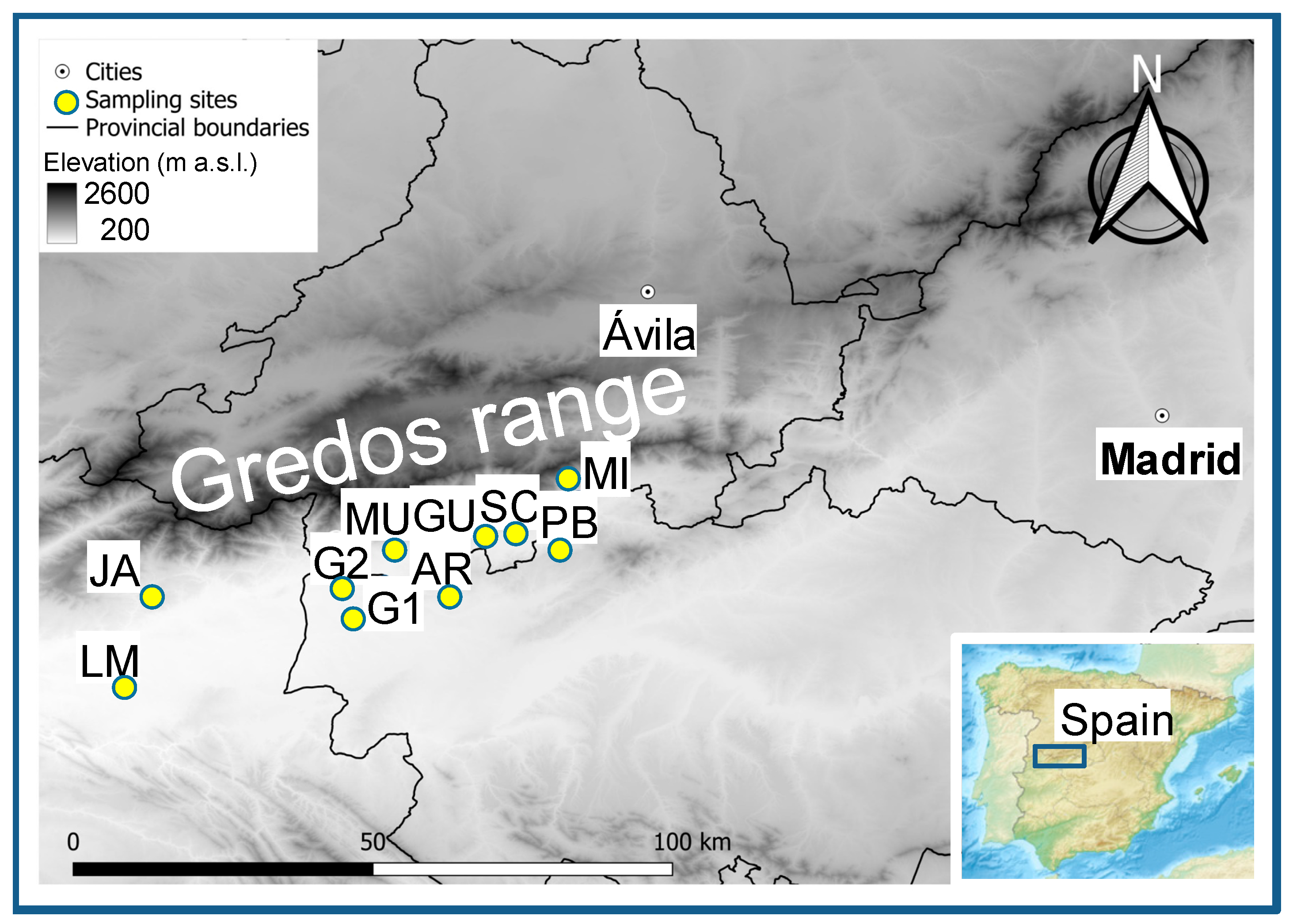
2.1. Study Sites and Tree Species

We sampled twelve sites located in the Sierra de Gredos, central Spain (Figure 1). Six tree species were selected for sampling (Table 1). Four sites corresponded to an evergreen conifer species, whereas the remaining eight sites were dominated by five hardwood species (two evergreen species plus three deciduous species). The climate of the studied region is Mediterranean continental with cold-wet winters and warm-dry summers [8]. The mean annual temperature is 14.5 °C, and the mean maximum and minimum temperatures are 30.1 °C and 0.0 °C, respectively. The total annual precipitation is 1483 mm (data from “Arenas de San Pedro” meteorological station; 5°5′28″ W, 40°12′31″ N, 510 m a.s.l.).
The vegetation of the study area is formed by oak and pine forests. The understory of these stands is dominated by several Mediterranean shrubs typical of sites with acidic soils such as Erica arborea L. or Cistus ladanifer L. Geological substrates are dominated by granite and gneiss, and soils are moderately deep at mid-elevation [9]. The resin tapping industry favored planting Pinus pinaster Ait. at low-to-mid elevations, particularly from the 1950s onwards [8]. This is considered a fire-resistant pine species due to its thick bark, among other traits [10,11].
All studied tree species are found across the western Mediterranean basin, except for Q. robur which reaches its southwestern distribution limit in this region [12]. They were selected because they are located along different situations of soil moisture gradients and form distinct, annual rings.
Pinus pinaster Ait. (Pinaceae) growth decreases as water deficit occurs during the growing season [13,14]. It is a shade-intolerant, fast-growing, isohydric, and drought-tolerant conifer found at low-to-mid elevations on acidic soils [15,16].
Quercus pyrenaica Willd. and Quercus robur L. (Fagaceae) are winter-deciduous, anisohydric oaks forming ring-porous wood. The first species is abundant in sites with continental and seasonally dry conditions with acidic soils and better tolerate drought than the second species, which abounds in lowland wet sites of N and NW Spain [17,18]. Q. robur reaches its southern limit in Spain on the southern slopes of the Sierra de Gredos.
Quercus ilex subsp. ballota (Desf.) Samp or Quercus rotundifolia Lam. (Fagaceae), hereafter Q. ilex, is the most important and widely naturally distributed broadleaf species in the Iberian Peninsula. It is an evergreen, shade-tolerant, anisohydric oak forming diffuse to semi-ring-porous wood [19].
Prunus lusitanica L. (Rosaceae) is a Mediterranean shade-tolerant evergreen species, usually found growing as a small tree or shrub (3–10 m) near small rivers or streams and forming mid-size leaves and diffuse-porous wood. This anisohydric species forms relict, isolated populations restricted to small valleys and mid slopes with northern aspects where microclimate conditions allow high soil moisture levels [20]. P. lusitanica is a Tertiary relict, being threatened by aridification and human impacts [21].
Celtis australis L. (Ulmaceae) is a Mediterranean, shade-intolerant, fast-growing deciduous tree species forming ring-porous wood, abundant in locations with access to shallow soil water such as close to streamsides [5,22]. It is considered an anisohydric species.
Both P. lusitanica and C. australis are often considered riparian species and are found near streamsides and gorges where high soil moisture buffers summer drought stress. In these wet locations, other tree species typical of mesic and riparian habitats also appear (e.g., Castanea sativa Mill., Fraxinus angustifolia Vahl. and Alnus glutinosa (L.) Gaertn.) (currently named Alnus lusitanica Vít., Douda & Mandák). Some of these species (C. australis, F. angustifolia) are considered phreatophytes because they uptake most water from the saturated zone [23]. In the study area, tree growth is enhanced by wet-cool climate conditions during winter and the growing season, which are driven by negative phases of the North Atlantic Oscillation [16,24,25].

2.2. Climate Data and Indices

We used monthly climate data (Tmax, mean maximum temperature; Tmin, mean minimum temperature; Prec, total precipitation) from the 0.1°-gridded E-OBS v23.1e dataset [26]. These long-term, homogeneous data were downloaded using the Climate Explorer web portal (http://climexp.knmi.nl, accessed on 3 March 2025). We also obtained monthly North Atlantic Oscillation (NAO) indices from the CRU webpage (https://crudata.uea.ac.uk/cru/data/nao/, accessed on 3 March 2025). The NAO indices reflect changes in sea level pressure in the North Atlantic region, which affect westerly winds reaching the Iberian Peninsula and bringing moist fronts in winter [27]. Positive NAO indices are linked to dry and warm winter-to-spring conditions in central and western Spain [28].

2.3. Field Sampling

In the field, we selected dominant, mature, apparently healthy trees of each dominant species in each site. We sampled several sites in some species (P. pinaster, 4 sites; Q. pyrenaica, P. lusitanica, and C. australis, 2 sites of each species) to encompass environmental variability or different disturbance regimes. First, we sampled several P. pinaster stands, located on rocky sites but subjected to different disturbance histories of tapping, fires, and logging as indicated by the difference in size. Tapping scars were observed in pines sampled in Pedro Bernardo (PB) and Guisando (GU) sites, whereas fire scars were found in some trees from the Santa Cruz del Valle (SC) site. Logging impacts (stumps, gaps) were common in all pine stands except in SC. Second, we sampled two sites where Q. pyrenaica and P. lusitanica stands were found in nearby locations (50 m apart) but with P. lusitanica being restricted to gorges and streamsides. In site MU (Río Muelas), P. lusitanica individuals were growing very close to the stream. Most P. lusitanica individuals were multi-stemmed. The sampled Q. pyrenaica trees were relatively young and small, characteristic of secondary forests occupying formerly cultivated lands or pastures. Third, two C. australis stands showing different stand structures and climate conditions were also sampled. They were characterized by small size and rocky substrates (site G1) and bigger size (site G2), respectively. In both sites, C. australis coexisted with ash (F. angustifolia) and scattered Q. ilex trees.
Regarding the two oak species with one site per species, the Q. robur sample stand was part of an open woodland located near a river, and it constitutes one of the southernmost populations of the species distribution area across Europe [18]. We paid particular attention to sample Q. robur individuals with leaf and acorn characters of the species since this oak often hybridized with Q. pyrenaica. In the case of the sampled Q. ilex trees, they corresponded to a savanna-like “dehesa” formation, which is an anthropogenic agroforestry formation where grasslands and trees are exploited for pasture and timber or acorns, respectively.
Field sampling consisted of measuring the diameter of the thickest stems of each individual at 1.3 m (dbh, diameter at breast height) and extracting two cores at the same height, perpendicular to the maximum slope, using 5 mm Pressler increment borers. At each site, 10 to 20 individuals were sampled (Table 2).

2.4. Processing Wood Samples and Ring-Width Data

Dendrochronology was used to process the wood samples, measure growth rates, and quantify climate–growth relationships [3,29]. Wood cores were air-dried, glued onto supports, and sanded with sandpapers of finer grain until ring limits were conspicuous. Then, samples were visually cross-dated under the stereomicroscope. Ring widths were measured with a 0.001 mm resolution along two cores per tree. This was done on images scanned at a resolution of 2400 dpi. Measurements were carried out using the CooRecorder-CDendro software (v. 9.8.1, Saltsjöbaden, Sweden) [30]. The cross-dating of samples was further checked using the COFECHA software version 6.06P, which calculates moving correlations between individual and mean series of ring-width indices for each site and species [31].
To compare growth rates between species of the same sites, we converted the ring-width series into basal-area increment (BAI) series, which is a more accurate measure of growth [32]. The BAI series were calculated using the following equation and assuming concentric growth:
BAI = π (R2tR2t−1)
where R2t and R2t−1 are the radii corresponding to the current (t) and prior (t − 1) years, respectively, and π is the pi number. The radii are calculated as the sums of tree-ring widths (RW) from year 1 up to years t ( 1 t R W ) and t − 1 ( 1 t 1 R W ), respectively.
To calculate climate–growth relationships, a series of ring-width data were converted into ring-width indices through detrending and standardization [3,29]. This allowed us to remove growth trends due to changes in stem age. Detrending was done by fitting polynomial splines of 2/3 of the growth series length and a 0.5 response cut-off to preserve annual to decadal growth variability. Then, autoregressive models were fitted to each detrended series to remove most of the first-order autocorrelation. The resulting pre-whitened or residual series of ring-width indices (RWI) were averaged by using bi-weight robust means to obtain mean series or chronologies for each site and species.
Several tree-ring statistics were calculated to characterize raw and indexed series over the common period 1970–2021 [33]. These statistics included: the first-order autocorrelation of raw ring widths (AR1), the mean sensitivity (MSx) of standardized indices, which measures relative changes in ring width between consecutive rings, and the mean correlation among indexed ring-width series (Rbar). Then, we calculated the Expressed Population Signal (EPS) to assess how well replicated and how coherent the obtained chronologies were [34]. The processing of tree-ring width series was done using the package dplR [35,36] in the R statistical software ver. 4.4.2 [37].

2.5. Statistical Analyses

First, we compared ring-width statistics between sites or species using Mann–Whitney U tests given that some variables did not follow normality according to Shapiro–Wilk tests. Second, the BAI trends were assessed using Mann–Kendall S tests. Third, a Principal Component Analysis (PCA) was performed considering the best-replicated period (1970–2021) to summarize the common variability among ring-width series. The PCAs were based on the variance–covariance matrix of the residual chronologies. We considered the first (PC1) and second (PC2) principal components because they accounted for at least 50% of the variance. The PCA was calculated using the function rda of the vegan R package version 2.7-0. [38]. Fourth, to obtain climate–growth relationships, Pearson correlations were calculated between monthly climate data (TMax, mean maximum temperature; TMin, mean minimum temperature; Prec, total precipitation) or NAO indices and the PC1 and PC2 scores (period 1970–2021). We considered the temporal window from the previous October to the current September. The climate–growth relationships were calculated using the treeclim R package [39]. Linear regressions were fitted to a series of ring-width indices as a function of May–June precipitation.
To precisely define the temporal window, during which the relationship between a monthly climate variable and growth indices is maximum, we used the R package climwin, which provides more robust results than simple correlations [40,41]. Climwin allows for comparing multiple models, which are ranked using the corrected Akaike Information Criterion (AICc) and calculates their R2 and significance levels. The difference between the AICc of the selected model and that of the baseline model (ΔAICc) is minimized [42]. Then, randomization tests are used to calculate the probability value (p AICc) that determines the likelihood that the ΔAICc value of the selected model has occurred by chance. We assumed linear relationships between climate and growth variables following [43,44]. Randomization tests demand computational power. Thus, we used the “Magerit” high-performance computer (Univ. Politécnica de Madrid, www.cesvima.upm.es, Spain, last accessed on 24 February 2025) to perform them. More details regarding this method can be found in Rubio-Cuadrado et al. [43].

3. Results

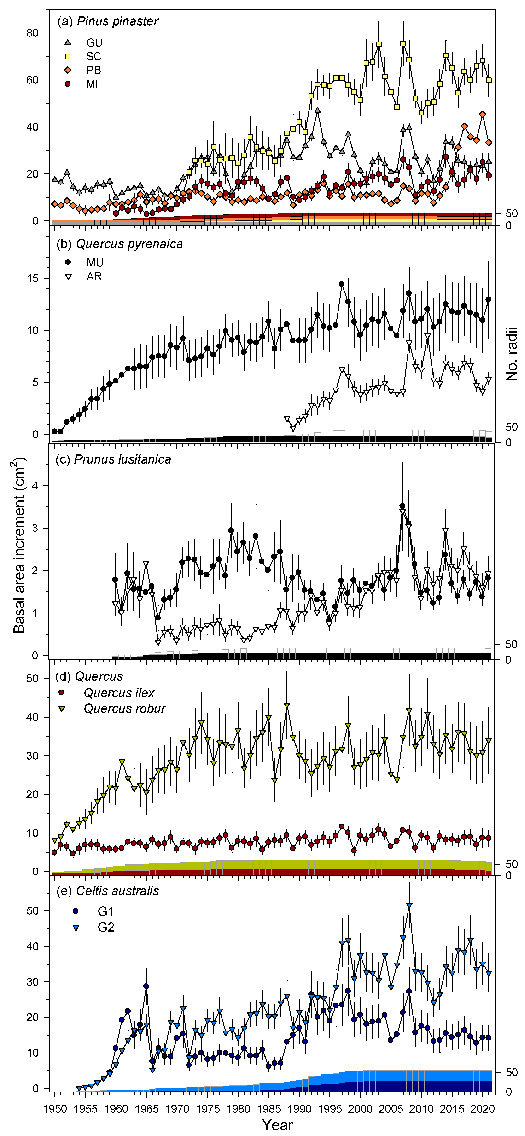
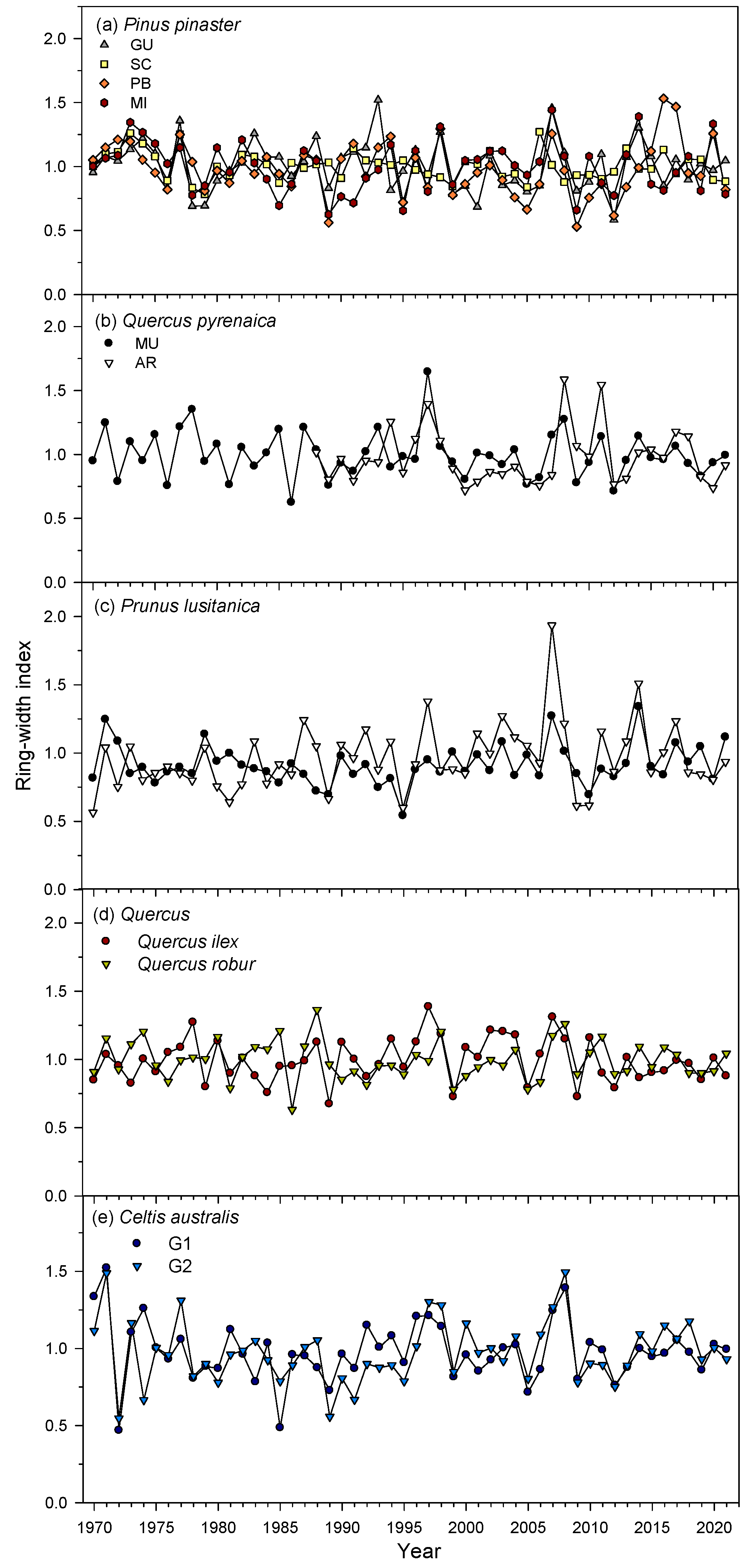
3.1. Growth Trends and Variability

We found great variability in growth trends and rates between and within species (Figure 2, Table 2). In P. pinaster, the site SC dominated by young, fast-growing trees, showed the highest BAI values, whereas older stands showed the lowest values (PB, MI). In Q. pyrenaica, site MU showed higher BAI values than site AR, but no differences in BAI were found between the two P. lusitanica sites, particularly after the 1995 drought. In the other oak species, BAI values were much higher in Q. robur than in Q. ilex (32.2 vs. 8.1 cm2, respectively). Finally, in C. australis, BAI was higher at site G2 than at site G1.
Regarding tree-ring statistics, P. pinaster, Q. robur, and C. australis showed the widest rings and highest BAI values, whereas P. lusitanica and Q. ilex showed the narrowest rings (Table 2). The BAI trends were positive and significant in all sites, except for the P. lusitanica MU site. Q. ilex presented the lowest AR1 value, whilst P. pinaster (site SC) showed the highest one. The lowest and highest MSx values corresponded to Q. robur and P. lusitanica (site AR), respectively, whereas the lowest and highest Rbar values were found for P. lusitanica and Q. pyrenaica (both being located in site AR), respectively. All chronologies were well replicated (EPS > 0.85), except for the two P. lusitanica sites, which showed a lower internal coherence between conspecific trees than the other species.
The correlations between series of ring-width indices of the same species (Figure 3), considering the period 1970–2021, decreased in the following order: C. australis (r = 0.81, p < 0.001) > Q. pyrenaica (r = 0.71, p < 0.001) > P. lusitanica (r = 0.58, p < 0.001) > P. pinaster (r = 0.55, p < 0.001, sites PB and GU). Remarkably, Q. ilex and Q. robur ring-width series showed a positive and significant correlation (r = 0.31, p = 0.03).
The first and second components of the PCA accounted for 42.22% (PC1) and 13.74% (PC2) of the growth variability, respectively. The PCA biplot showed that chronologies of the same species were grouped together, as were those of Q. ilex and Q. robur (Figure 4). As found with correlations between chronologies, P. pinaster (site MI) and Q. pyrenaica (site AR) appeared separated in the biplot and showed opposite scores along the PC2 axis. The species’ series of growth indices more strongly correlated with the PC1 scores were those of P. lusitanica and C. australis from sites AR and G2, respectively. The P. pinaster series showed strong positive correlations with the PC2 scores, particularly at site MI, whereas the Q. pyrenaica series showed negative correlations, particularly at site AR. The years’ scores indicated high growth indices in 1971, 1997, 2007, and 2008 but low growth indices in 1989, 1995, 2009, and 2012.

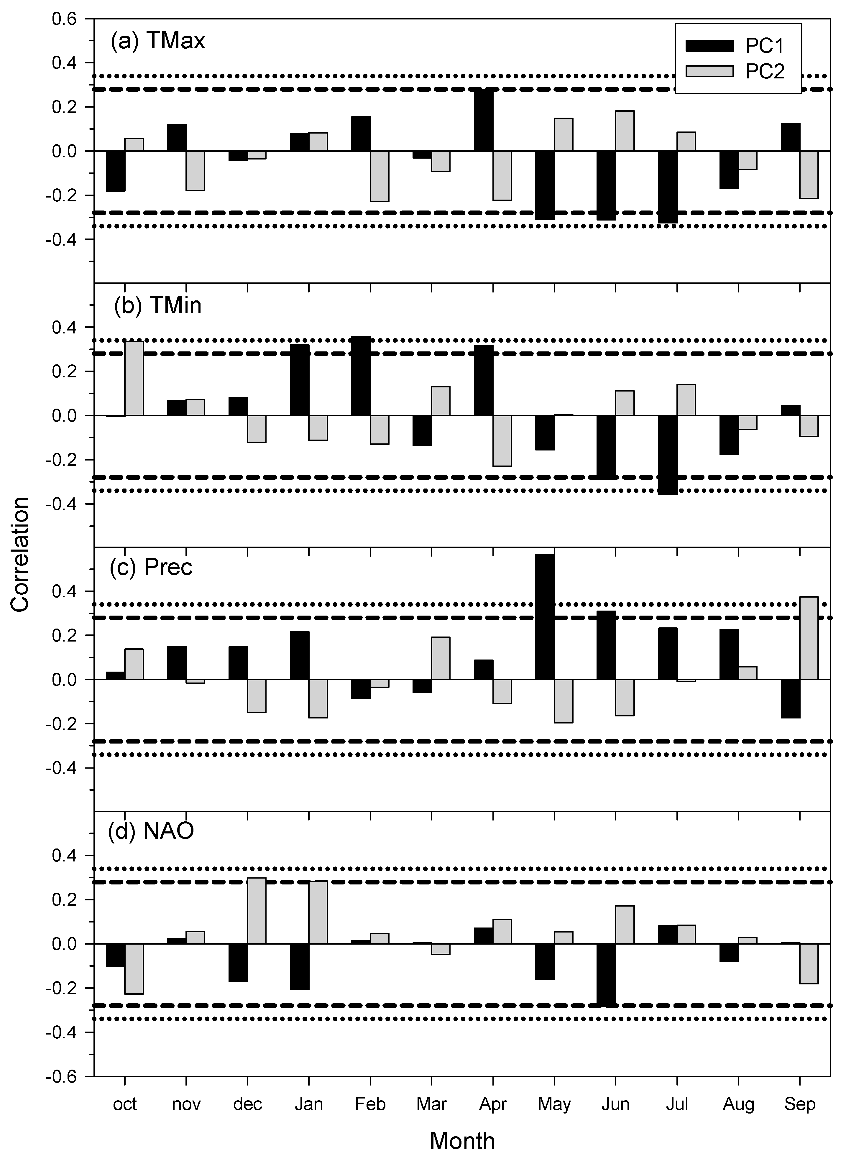
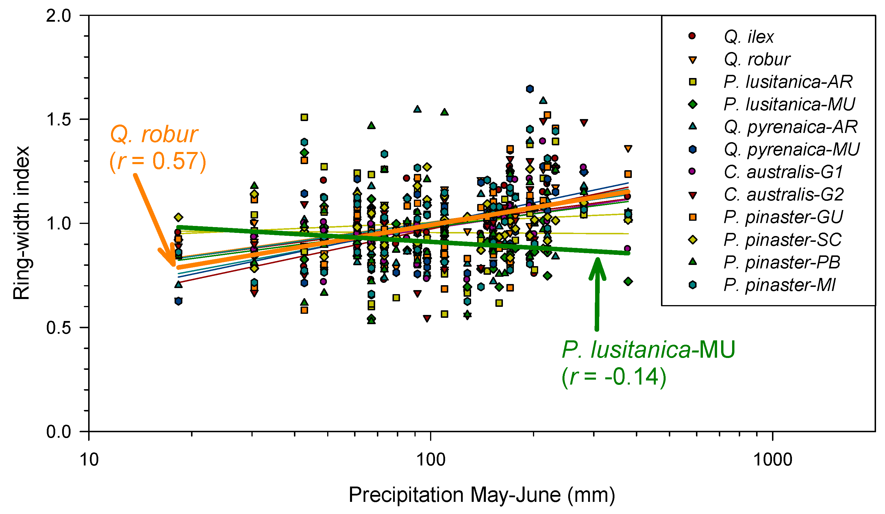
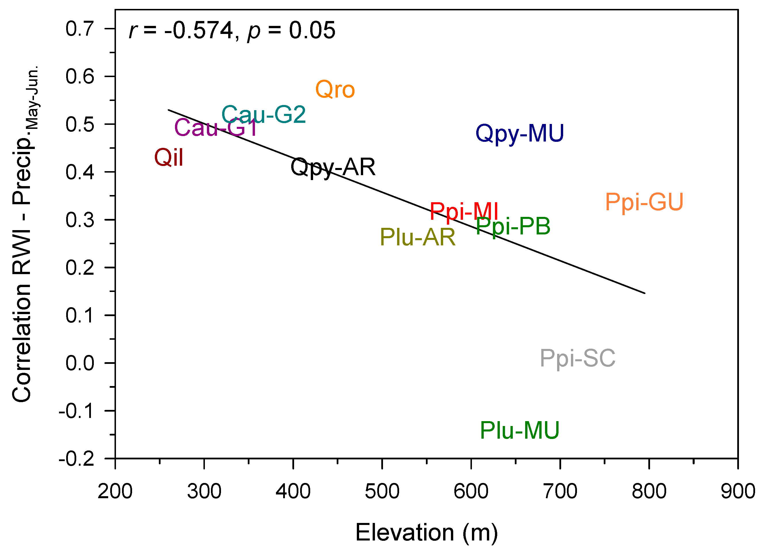
3.2. Correlations Between Climate Variables and Growth Indices

The correlations between monthly climate variables or NAO indices and the PC1 and PC2 scores indicated that the PC1 scores increased as May and June precipitation increased (Figure 5). This means that the PC1 axis was driven by growing-season precipitation. Warm conditions in the prior winter and in the current spring also showed positive associations with PC1, but temperatures in the June–July or June NAO indices showed negative correlations. In the case of PC2, warm conditions in the prior autumn and wet conditions in the current early autumn enhanced it. NAO indices in December–January correlated positively with PC2 scores. The December–January NAO indices also showed a positive correlation with the mean series of Q. pyrenaica growth indices (r = 0.34, p = 0.01).
The dominant role played by May–June precipitation on growth variability allowed the species’ and sites’ chronologies to be ranked (Figure 6). We found that the highest and lowest precipitation–growth correlations corresponded to Q. robur and P. lusitanica (site MU), respectively.
The relationship between growth indices and May–June precipitation increased as site elevation decreased (r = −0.57, p = 0.05). The strongest precipitation–growth coupling appeared in warmer and drier sites dominated by C. australis and oak species (Figure 7).

3.3. Climate–Growth Relationships Based on Climwin Analyses

Climwin confirmed that growing-season precipitation was the key climatic driver of growth variability, particularly in the case of oak species and C. australis, being significant (p < 0.05) in all sites and species, except in the P. lusitanica site MU (Table 3). The highest R2 values corresponded to precipitation (e.g., Q. robur) and randomization tests were significant (pAICc < 0.05) in most cases, except in P. lusitanica (sites AR and MU) and P. pinaster (sites SC, MI, and GU). In the two deciduous oak species and also in C. australis, the temporal window of precipitation included May to August. However, in Q. ilex and in the P. pinaster PB site, the window included the previous August to the current September. Temperatures also showed high R2 values for some P. pinaster (GU, PB) and oaks’ sites, except Q. pyrenaica at site AR. In Q. ilex and Q. robur, the window of minimum temperatures spanned from January to March, whilst in the Q. pyrenaica site MU, temperatures were more important from June to July. In the P. pinaster PB and GU sites, the temporal window of minimum temperatures went from May to November.

4. Discussion

As hypothesized, those tree species located in microsites with high soil moisture levels, such as near streamsides or gorges, showed the weakest growth responses to growing-season precipitation, the major driver of growth in the studied Mediterranean mountainous region. This was particularly evident for the understudied P. lusitanica, a Tertiary relic tree that forms scattered populations in wet refuges near rivers [20]. Interestingly, the drought-tolerant P. pinaster also showed low correlations with water availability. First, this can be explained by influences of other climatic factors such as minimum temperatures. For instance, in the same study area, it was found that P. pinaster radial growth was enhanced by warm winter temperatures [16,24]. Thus, both low temperatures before the growth onset and water deficit constrain P. pinaster growth and affect its wood density [45]. Second, we sampled pine stands showing diverse age and size structures and subjected to different disturbance regimes. Formerly tapped P. pinaster trees are more sensitive to drought stress [46], and this could explain the higher precipitation–growth correlations obtained for sites PB and GU as compared with sites SC and MU.
The BAI trend analyses indicated that the highest increases in wood production corresponded to the Q. pyrenaica MU site, the C. australis G2 site, the P. pinaster PB site, and the Q. robur and Q. ilex sites. Overall, this indicates that anisohydric, winter-deciduous (Q. pyrenaica, Q. robur, C. australis) or evergreen (Q. ilex) tree species showed the strongest growth enhancements. The recent BAI surge observed in the formerly tapped P. pinaster PB site could be a response to improved climatic conditions, i.e., higher soil moisture. Considering their respective hydrological niches, the sites showing the strongest increases in wood production occupied intermediate (e.g., Q. pyrenaica, Q. ilex) situations or were located near river sites (e.g., C. australis, Q. robur). The riparian P. lusitanica site (MU) showing the lowest growth sensitivity to precipitation was among the wettest locations. Nevertheless, it showed a negative BAI trend indicating that wet conditions do not improve wood production in this species. This pattern may also be influenced by tree size because P. lusitanica showed the lowest diameter and BAI values.
The highest precipitation–growth correlation corresponds to Q. robur. In this sense, among the species most sensitive to changes in water availability, climwin analyses highlighted deciduous (Q. robur, Q. pyrenaica) and evergreen (Q. ilex) oaks, and also C. australis. Oaks are anisohydric species, showing a rapid post-drought recovery [47], perhaps through the use of abundant stored carbohydrates or by accessing deep water sources during late summer, but a low resistance to drought, which leads to severe growth reductions and reduces vessel lumen area [17,19]. Moreover, they also showed sensitivity to cold winter conditions and elevated temperatures, increasing vapor pressure deficit. These results indicate that hot and lasting drought conditions could threaten the persistence of some individuals in the sampled marginal, rear-edge Q. robur population. In addition, warm winter conditions linked to positive NAO phases seem to be related to the enhanced growth of Q. pyrenaica, which contrasts with findings on pine species in the same study area showing a growth reduction associated with dry winter conditions and negative NAO phases [16,24]. In the case of C. australis, previous studies evidenced that the growth of this riparian, phreatophytic species is very dependent on spring water availability [5,22]. Therefore, wet and cool conditions from May to June enhanced the growth of this species, and the forecasted aridification trends would negatively impact this species if accompanied by hydrological droughts.
In the case of P. lusitanica, its growth only showed a weak positive response to warmer conditions in the prior autumn and the current growing season. This paleotropical relict species requires high levels of air and soil moisture and is only found near riparian habitats (streamsides or gorges), which represent its main climatic refuges [21,48,49]. Despite P. lusitanica and C. australis sharing some functional traits (big leaves, high wood density, use of shallow water sources) and habitat preferences (riparian habitats), they presented very contrasting responses to precipitation. This suggests that they did not have the same hydrological niche and that there could be vertical segregation in the use of soil water and nutrients, with C. australis using deeper sources during the late summer to alleviate drought stress.
Lastly, we acknowledge that no direct measurements of soil water availability or indirect measures of water-use efficiency (e.g., wood C isotope discrimination) or soil water use (H and O isotope discrimination in soil and xylem water samples) were considered. Undoubtedly, these variables would have contributed to improving our assessments of the hydrological niche and should be considered in future research efforts.
At least two major limitations affected our analyses. First, the climate–growth relationships could be influenced by the low age of some stands. For instance, the low age of Q. pyrenaica individuals sampled in site AR resulted in secondary succession after land abandonment started in the 1960s. To overcome this limitation, older stands should be explored and sampled. Second, the disturbance regime may also distort topography–climate–growth relationships, as observed in the case of P. pinaster. To solve this limitation, stands with similar disturbance regimes (e.g., tapping) could be compared or the disturbance history should be explicitly integrated into the analyses of the climate–growth relationships [46].

5. Conclusions

Climate variability at regional to local scales differently impacted tree radial growth along the soil moisture gradient. The tree-ring responses to regional climate depended on the species’ hydrological niche. We used tree-ring data and calculated climate–growth relationships to disentangle the hydrological niche of tree species across a complex topographical area. The Mediterranean climate conditions of the study area, characterized by a severe summer drought, explained that most species and sites showed high growth responsiveness to growing-season precipitation. However, this responsiveness increased as elevation decreased, indicating a topographic and species-dependent modulation of soil water use. This gradient was characterized by two opposite extremes with low-elevation sites of oaks and C. australis sites being characterized by strong moisture-growth associations, and mid-elevation P. pinaster and P. lusitanica sites showing a lower dependence on precipitation. Several reasons may explain the precipitation–growth uncoupling such as disturbance regime (P. pinaster) or species restricted to riparian refuges providing consistently high soil moisture levels (P. lusitanica). Our findings illustrate the complex inferences derived from tree-ring analyses but also reveal the potential to refine the hydrological niche of tree species by using a long-term series of climate and radial growth. This improvement is based on a temporal characterization of the hydrological niche.

Author Contributions

Conceptualization, J.J.C., Á.R.-C. and J.A.L.S.; methodology, J.J.C., Á.R.-C., J.A.L.S., E.G.d.A., M.C., D.A.-S., A.C.-V., Ó.P.-P. and C.V.; software, J.J.C., Á.R.-C. and C.V.; validation, J.J.C.; formal analysis, J.J.C., J.A.L.S. and Á.R.-C.; investigation, J.J.C., J.A.L.S., Á.R.-C., D.A.-S. and C.V.; resources, J.J.C., Á.R.-C., J.A.L.S., D.A.-S. and C.V.; data curation, J.J.C. and C.V.; writing—original draft preparation, J.J.C.; writing—review and editing, J.J.C., Á.R.-C., J.A.L.S., D.A.-S., E.G.d.A., M.C., A.C.-V., Ó.P.-P. and C.V.; visualization, J.J.C. and Á.R.-C.; supervision, J.J.C. and J.A.L.S.; project administration, J.J.C.; funding acquisition, J.J.C. and D.A.-S. All authors have read and agreed to the published version of the manuscript.

Funding

This research was funded by the Spanish Ministry of Science and Innovation (grants PID2021-123675OB-C43, TED2021-129770B-C21, and TED2021-132631B-I00 funded by MICIU/AEI/ 10.13039/501100011033 and by NextGenerationEU/PRTR).

Data Availability Statement

Dataset available upon reasonable request from the authors.

Acknowledgments

We thank “Castilla y León” forest guards and technicians for their help during field sampling in Gredos. The authors gratefully acknowledge the Universidad Politécnica de Madrid for providing computing resources on the “Magerit” supercomputer (www.cesvima.upm.es, accessed on 3 March 2025).

Conflicts of Interest

The authors declare no conflicts of interest.

References

  1. Pan, Y.; Birdsey, R.A.; Fang, J.; Houghton, R.; Kauppi, P.E.; Kurz, W.A.; Phillips, O.L.; Shvidenko, A.; Lewis, S.L.; Canadell, J.G.; et al. A large and persistent carbon sink in the world’s forests. Science 2011, 333, 988–993. [Google Scholar] [CrossRef]
  2. Babst, F.; Bouriaud, O.; Poulter, B.; Trouet, V.; Girardin, M.P.; Frank, D.C. Twentieth century redistribution in climatic drivers of global tree growth. Sci. Adv. 2019, 5, eaat4313. [Google Scholar] [CrossRef]
  3. Fritts, H.C. Tree Rings and Climate; Academic Press: London, UK, 1976. [Google Scholar]
  4. Silvertown, J.; Araya, Y.; Gowing, D. Hydrological niches in terrestrial plant communities: A review. J. Ecol. 2015, 103, 93–108. [Google Scholar] [CrossRef]
  5. Camarero, J.J.; Sánchez-Salguero, R.; Sangüesa-Barreda, G.; Matías, L. Tree species from contrasting hydrological niches show divergent growth and water-use efficiency. Dendrochronologia 2018, 52, 87–95. [Google Scholar] [CrossRef]
  6. Kunz, J.; Löffler, G.; Bauhus, J. Minor European broadleaved tree species are more drought-tolerant than Fagus sylvatica but not more tolerant than Quercus petraea. For. Ecol. Manag. 2018, 414, 15–27. [Google Scholar] [CrossRef]
  7. Fuchs, S.; Schuldt, B.; Leuschner, C. Identification of drought-tolerant tree species through climate sensitivity analysis of radial growth in Central European mixed broadleaf forests. For. Ecol. Manag. 2021, 494, 119287. [Google Scholar] [CrossRef]
  8. López-Sáez, J.A.; Alba-Sánchez, F.; Sánchez-Mata, D.; Luengo-Nicolau, E. Los Pinares de la Sierra de Gredos. Pasado, Presente y Futuro; Institución Gran Duque de Alba: Ávila, Spain, 2019. [Google Scholar]
  9. Gallardo, J.F.; Cuadrado, S.Y.; González-Hernández, M.I. Suelos Forestales de la Vertiente sur de la Sierra de Gredos; VII Anuario del Centro de Edafología y Biología Aplicada de Salamanca: Salamanca, Spain, 1980; pp. 155–168. [Google Scholar]
  10. Fernandes, P.M.; Vega, J.A.; Jiménez, E.; Rigolot, E. Fire resistance of European pines. For. Ecol. Manag. 2008, 256, 246–255. [Google Scholar] [CrossRef]
  11. Tapias, R.; Climent, J.; Pardos, J.A.; Gil, L. Life histories of Mediterranean pines. Plant Ecol. 2004, 171, 53–68. [Google Scholar] [CrossRef]
  12. Caudullo, G.; Welk, E.; San-Miguel-Ayanz, J. Chorological maps for the main European woody species. Data Brief 2017, 12, 662–666. [Google Scholar] [CrossRef]
  13. Bogino, S.M.; Bravo, F. Growth response of Pinus pinaster Ait. to climatic variables in central Spanish forests. Ann. For. Sci. 2008, 65, 506. [Google Scholar] [CrossRef]
  14. Camarero, J.J.; Gazol, A.; Tardif, J.C.; Conciatori, F. Attributing forest responses to global-change drivers: Limited evidence of a CO2-fertilization effect in Iberian pine growth. J. Biogeogr. 2015, 42, 2220–2233. [Google Scholar] [CrossRef]
  15. Sánchez-Salguero, R.; Camarero, J.J.; Rozas, V.; Génova, M.; Olano, J.M.; Arzac, A.; Linares, J.C. Resist, recover or both? Growth plasticity in response to drought is geographically structured and linked to intraspecific variability in Pinus pinaster. J. Biogeogr. 2018, 45, 1126–1139. [Google Scholar] [CrossRef]
  16. Hernández-Alonso, H.; Madrigal-González, J.; Silla, F. Differential growth responses in Pinus nigra, P. pinaster and P. sylvestris to the main patterns of climatic variability in the western Mediterranean. For. Ecol. Manag. 2021, 483, 118921. [Google Scholar] [CrossRef]
  17. Corcuera, L.; Camarero, J.J.; Sisó, S.; Gil-Pelegrín, E. Radial-growth and wood-anatomical changes in overaged Quercus pyrenaica coppice stands: Functional responses in a new Mediterranean landscape. Trees Struct. Funct. 2006, 20, 91–98. [Google Scholar] [CrossRef]
  18. Moracho, E.; Moreno, G.; Jordano, P.; Hampe, A. Unusually limited pollen dispersal and connectivity of Pedunculate oak (Quercus robur) refugial populations at the species’ southern range margin. Mol. Ecol. 2016, 25, 3319–3331. [Google Scholar] [CrossRef]
  19. Campelo, F.; Gutiérrez, E.; Ribas, M.; Sánchez-Salguero, R.; Nabais, C.; Camarero, J.J. The facultative bimodal growth pattern in Quercus ilex—A simple model to predict sub-seasonal and inter-annual growth. Dendrochronologia 2018, 49, 77–88. [Google Scholar] [CrossRef]
  20. Beltrán, R.S. Distribución y autoecología de Prunus lusitanica L. en la Península Ibérica. Investig. Agraria. Sist. Recur. For. 2006, 15, 187–198. [Google Scholar]
  21. Pardo, A.; Cáceres, Y.; Pulido, F. Rangewide determinants of population performance in Prunus lusitanica: Lessons for the contemporary conservation of a Tertiary relict tree. Acta Oecol. 2018, 86, 42–48. [Google Scholar] [CrossRef]
  22. Garfi, G. Climatic signal in tree–rings of Quercus pubescens s.l. and Celtis australis L. in South–eastern Sicily. Dendrochronologia 2000, 18, 41–51. [Google Scholar]
  23. Naumburg, E.; Mata-Gonzalez, R.; Hunter, R.G.; Mclendon, T.; Martin, D.W. Phreatophytic vegetation and groundwater fluctuations: A review of current research and application of ecosystem response modeling with an emphasis on great basin vegetation. Environ. Manag. 2005, 35, 726–740. [Google Scholar] [CrossRef]
  24. Camisón, A.; Silla, F.; Camarero, J.J. Influences of the atmospheric patterns on unstable climate-growth associations of western Mediterranean forests. Dendrochronologia 2016, 40, 130–142. [Google Scholar] [CrossRef]
  25. Camarero, J.J.; Sangüesa-Barreda, G.; Montiel-Molina, C.; Seijo, F.; López-Sáez, J.A. Past growth suppressions as proxies of fire incidence in relict Mediterranean black pine forests. For. Ecol. Manag. 2018, 413, 9–20. [Google Scholar] [CrossRef]
  26. Cornes, R.C.; van der Schrier, G.; van den Besselaar, E.J.M.; Jones, P.D. An Ensemble Version of the E-OBS Temperature and Precipitation Data Sets. J. Geophys. Res. Atmos. 2018, 123, 9391–9409. [Google Scholar] [CrossRef]
  27. Hurrell, J. Decadal trends in North Atlantic Oscillation and relationship to regional temperature and precipitation. Science 1995, 269, 676–679. [Google Scholar] [CrossRef]
  28. Rodó, X.; Baert, E.; Comín, F. Variations in seasonal rainfall in Southern Europe during the present century: Relationships with the North Atlantic Oscillation and the El Niño-Southern Oscillation. Clim. Dyn. 1997, 13, 275–284. [Google Scholar] [CrossRef]
  29. Cook, E.R.; Kairiukstis, L.A. (Eds.) Methods of Dendrochronology: Applications in the Environmental Sciences; IIASA: Dordrecht, The Netherlands, 1990. [Google Scholar]
  30. Maxwell, R.S.; Larsson, L.-A. Measuring tree-ring widths using the CooRecorder software application. Dendrochronologia 2021, 67, 125841. [Google Scholar] [CrossRef]
  31. Holmes, R.L. Computer-assisted quality control in tree-ring dating and measurement. Tree-Ring Bull. 1983, 43, 68–78. [Google Scholar]
  32. Biondi, F.; Qeadan, F. A theory-driven approach to tree-ring standardization: Defining the biological trend from expected basal area increment. Tree-Ring Res. 2008, 64, 81–96. [Google Scholar] [CrossRef]
  33. Briffa, K.R.; Jones, P.D. Basic chronology statistics and assessment. In Methods of Dendrochronology: Applications in the Environmental Sciences; Cook, E.R., Kairiukstis, L.A., Eds.; Kluwer: Dordrecht, The Netherlands, 1990; pp. 439–461. [Google Scholar]
  34. Wigley, T.M.L.; Briffa, K.R.; Jones, P.D. On the average value of correlated time series, with applications in dendroclimatology and hydrometeorology. J. Clim. Appl. Meteorol. 1984, 23, 201–213. [Google Scholar] [CrossRef]
  35. Bunn, A.G. Statistical and visual crossdating in R using the dplR library. Dendrochronologia 2010, 28, 251–258. [Google Scholar] [CrossRef]
  36. Bunn, A.G.; Korpela, M.; Biondi, F.; Campelo, F.; Mérian, P.; Qeadan, F.; Zang, C. dplR: Dendrochronology Program Library in R. R Package, Version 1.7.8. 2025. Available online: https://cran.r-project.org/web/packages/dplR/index.html (accessed on 21 February 2025).
  37. R Core Team. A Language and Environment for Statistical Computing; R Foundation for Statistical Computing: Vienna, Austria, 2024; Available online: https://www.r-project.org/ (accessed on 21 February 2025).
  38. Oksanen, J.; Simpson, G.; Blanchet, F.; Kindt, R.; Legendre, P.; Minchin, P.R.; O’Hara, R.B.; Solymos, P.; Stevens, M.H.H.; Szoecs, E.; et al. Vegan: Community Ecology Package. R Package Version 2.7-0. 2025. [Google Scholar]
  39. Zang, C.; Biondi, F. Treeclim: An R package for the numerical calibration of proxy-climate relationships. Ecography 2015, 38, 431–436. [Google Scholar] [CrossRef]
  40. Bailey, L.D.; van de Pol, M. Climwin: An R Toolbox for Climate Window Analysis. PLoS ONE 2016, 11, e0167980. [Google Scholar] [CrossRef] [PubMed]
  41. van de Pol, M.; Bailey, L.D.; McLean, N.; Rijsdijk, L.; Lawson, C.R.; Brouwer, L. Identifying the Best Climatic Predictors in Ecology and Evolution. Methods Ecol. Evol. 2016, 7, 1246–1257. [Google Scholar] [CrossRef]
  42. Burnham, K.P.; Anderson, D.R. Model Selection and Multimodel Inference: A Practical Information-Theoretic Approach; Springer: New York, NY, USA, 2004; ISBN 978-0-387-95364-9. [Google Scholar]
  43. Rubio-Cuadrado, A.; Camarero, J.J.; Bosela, M. Applying climwin to dendrochronology: A breakthrough in the analyses of tree responses to environmental variability. Dendrochronologia 2022, 71, 125916. [Google Scholar] [CrossRef]
  44. Rubio-Cuadrado, Á.; Camarero, J.J. More than Just Chilling and Forcing: Deconstructing the Climate Windows and Drivers of Leaf Emergence and Fall in Woody Plant Species. Forests 2025, 16, 175. [Google Scholar] [CrossRef]
  45. Kurz-Besson, C.B.; Lousada, J.L.; Gaspar, M.J.; Correia, I.E.; David, T.S.; Soares, P.M.; Trigo, R.M. Effects of recent minimum temperature and water deficit increases on Pinus pinaster radial growth and wood density in southern Portugal. Front. Plant Sci. 2016, 7, 1170. [Google Scholar] [CrossRef]
  46. Fernández-Blas, C.; Ruiz-Benito, P.; Gazol, A.; Granda, E.; Samblás, E.; Granado-Díaz, I.; Zavala, M.A.; Valeriano, C.; Camarero, J.J. Historical forest use constrains tree growth responses to drought: A case study on tapped maritime pine (Pinus pinaster). Trees For. People 2024, 18, 100699. [Google Scholar] [CrossRef]
  47. Anderegg, W.R.L.; Schwalm, C.; Biondi, F.; Camarero, J.J.; Koch, G.; Litvak, M.; Ogle, K.; Shaw, J.D.; Shevliakova, E.; Williams, A.P.; et al. Pervasive drought legacies in forest ecosystems and their implications for carbon cycle models. Science 2015, 349, 528–532. [Google Scholar] [CrossRef]
  48. Pulido, F.; Valladares, F.; Calleja, J.A.; Moreno, G.; González-Bornay, G. Tertiary relict trees in a mediterranean climate: Abiotic constraints on the persistence of Prunus lusitanica at the eroding edge of its range. J. Biogeogr. 2008, 35, 1425–1435. [Google Scholar] [CrossRef]
  49. Raposo, M.A.M.; Nunes, L.J.R.; Quinto-Canas, R.; del Río, S.; Pardo, F.M.V.; Galveias, A.; Pinto-Gomes, C.J. Prunus lusitanica L.: An Endangered Plant Species Relict in the Central Region of Mainland Portugal. Diversity 2021, 13, 359. [Google Scholar] [CrossRef]
Figure 1. Map showing the location of the Sierra de Gredos range in Spain and the study sites.
Forests 16 01029 g001
Figure 2. Mean series of basal area increment calculated for each site and species ((a), P. pinaster; (b), Q. pyrenaica; (c), P. lusitanica; (d), Q. ilex and Q. robur; and (e), C. australis). Values are means ± SE. The bars show the annual sample sizes (number of measured radii, right y-axes). Different colors of symbols and bars correspond to different species or sites.
Forests 16 01029 g002
Figure 3. Series of ring-width indices (chronologies) calculated for each site and species ((a), P. pinaster; (b), Q. pyrenaica; (c), P. lusitanica; (d), Q. ilex and Q. robur; and (e), C. australis). Different colors of symbols and bars correspond to different species or sites.
Forests 16 01029 g003
Figure 4. PCA biplot showing the scores of the series of ring-width indices and the years. Sites’ codes are as in Table 1 but preceded by species’ abbreviations (Ppi, P. pinaster; Qpy, Q. pyrenaica; Qil, Q. ilex; Qro, Q. robur; Cau, C. australis; Plu, P. lusitanica). Only years’ scores of the common period (1970–2021) with PC1 > |0.1| and PC2 > |0.1| are represented. Symbols of different colors indicate different species and sites.
Forests 16 01029 g004
Figure 5. Correlations (Pearson coefficients) calculated between the PC1 (black bars) and PC2 (grey bars) scores and monthly climate variables or indices: (a) TMax, mean maximum temperature; (b) TMin, mean minimum temperature; (c) Prec, total precipitation; and (d) NAO, North Atlantic Oscillation index. Horizontal dashed and dotted lines indicate the 0.05 and 0.01 significance levels, respectively. Months abbreviated by lowercase and uppercase letters correspond to the previous and current years, respectively.
Forests 16 01029 g005
Figure 6. Linear regressions fitted to the series of ring-width indices as a function of summed precipitation from May to June (period 1970–2021). The arrows indicate the regressions with the highest (Q. robur, orange line) and lowest (P. lusitanica in site MU, green line) correlations, respectively. Sites’ codes are shown in Table 1. Note that the x-axis is a logarithmic scale. Symbols and lines of different colors indicate different species and sites.
Forests 16 01029 g006
Figure 7. Negative relationship found between site elevation and the correlation between growth indices (RWI) and the May-to-June precipitation (y-axis). The statistics show the Pearson correlation coefficient and its significance level, whereas the line shows the linear regression between both variables. Sites’ codes are as in Table 1 but preceded by species’ abbreviations (Ppi, P. pinaster; Qpy, Q. pyrenaica; Qil, Q. ilex; Qro, Q. robur; Cau, C. australis; Plu, P. lusitanica). The correlation threshold for significance (p < 0.05) is r > 0.27. Symbols of different colors indicate different species and sites.
Forests 16 01029 g007
Table 1. Characteristics of the study sites.
Tree SpeciesSite NameSite CodeLatitude N (°)Longitude W (°)Elevation (m a.s.l.)Sampling Date
Quercus ilexMajadas del TiétarLM39.94525.7683260July 2022
Quercus roburJaraíz de la VeraJA40.09555.7690447April 2022
Quercus pyrenaicaRío ArbillasAR40.18105.1497445October 2021
Quercus pyrenaicaRío MuelasMU40.18355.1907655October 2021
Prunus lusitanicaRío ArbillasAR40.18105.1497540October 2021
Prunus lusitanicaRío MuelasMU40.18355.1907655October 2021
Celtis australisOropesa G140.09835.2110314October 2023
Celtis australisCandeledaG240.13965.2516367October 2023
Pinus pinasterGuisandoGU40.21675.1417795January 2022
Pinus pinasterSanta Cruz del ValleSC40.20835.0167720January 2022
Pinus pinasterPedro BernardoPB40.21654.9332647January 2022
Pinus pinasterMijaresMI40.26174.8350592January 2022
Table 2. Size (dbh, diameter at breast height), age, and tree-ring statistics (AR1, first-order autocorrelation; MSx, mean sensitivity; Rbar, mean correlation among indexed ring-width series; EPS, Expressed Population Signal (EPS). The BAI trends were assessed using Mann–Kendall S tests (significance levels: ** p < 0.01, *** p < 0.001). Values are means ± SD. Different letters indicate significant (p < 0.05) differences between sites of the same species.
SpeciesSiteDbh (cm)Time SpanNo. Trees/No. CoresBAI (cm2)BAI Trend (S)Tree-Ring Width (mm)AR1MSxRbarEPS
Q. ilexLM48.9 ± 8.41927–202213/248.1 ± 1.41066 ***0.61 ± 0.110.510.350.430.86
Q. roburJA50.4 ± 14.01941–202120/4032.2 ± 4.51186 ***2.94 ± 0.960.710.220.590.92
Q. pyrenaicaAR18.6 ± 3.3 a1987–202110/204.7 ± 2.0 a307 **2.23 ± 0.58 a0.570.310.630.92
MU26.0 ± 3.4 b1941–202110/209.7 ± 2.0 b2012 ***1.63 ± 0.31 b0.680.270.490.89
P. lusitanicaAR12.8 ± 2.7 a1957–202111/181.3 ± 0.7 a941 ***0.92 ± 0.30 a0.560.400.330.79
MU15.4 ± 2.9 a1942–202113/231.9 ± 0.5 a−1330.94 ± 0.30 a0.680.360.390.80
C. australisG119.7 ± 4.8 a1958–202315/2914.9 ± 3.4 a423 **2.06 ± 1.11 a0.560.290.470.88
G239.1 ± 9.2 b1954–202315/2627.4 ± 6.3 b1674 ***3.16 ± 1.29 a0.550.310.450.87
P. pinasterGU66.5 ± 6.9 b1912–202115/3124.0 ± 7.2 a994 ***2.55 ± 0.77 a0.730.260.420.86
SC70.0 ± 8.0 b1968–202112/2352.1 ± 9.4 b817 ***6.44 ± 1.53 b0.760.250.610.89
PB49.0 ± 7.9 a1883–202112/2413.1 ± 6.3 a1342 ***1.82 ± 0.60 a0.730.300.450.87
MI47.0 ± 5.0 a1956–202115/2416.0 ± 4.4 a1049 ***2.80 ± 0.66 a0.680.310.620.90
Table 3. Models selected by climwin assuming linear relationships between growth indices and climate variables (Tmax, Tmin, and Prec: maximum and minimum temperatures and precipitation). The monthly climate window goes from previous years (t − 1) to the current year. Significant (p < 0.05) p AICc values are indicated with bold characters.
SpeciesSiteClimate Variable∆AICcWindow OpenWindow Closep ValueR2p AICc
Q.ilexLMTmax−1.71Aug (t − 1)Sep (t − 1)0.0520.0750.550
Tmin−11.36JanMar<0.0010.2340.013
Prec−13.65Aug (t − 1)Sep<0.0010.2680.006
Q.roburJATmax−6.91MayMay0.0030.1650.071
Tmin−12.1JanFeb<0.0010.2450.005
Prec−21.08MayJun<0.0010.367<0.001
Q. pyrenaicaARTmax−3.79AprApr0.0160.1120.287
Tmin−4.73JulJul0.0100.1280.224
Prec−8.59MayJun0.0010.1920.045
MUTmax−14.3JunJul<0.0010.2770.007
Tmin−12.63JunJul<0.0010.2530.007
Prec−15.93MayAug<0.0010.3000.003
P. lusitanicaARTmax−3.59MarApr0.0180.1080.282
Tmin−1.71JanApr0.0520.0750.648
Prec−6.6Sep (t − 1)Sep (t − 1)0.0040.1600.160
MUTmax−1.95Sep (t − 1)Sep (t − 1)0.0450.0790.537
Tmin−3.66Sep (t − 1)Sep (t − 1)0.0180.1100.328
Prec−0.78JulOct0.0890.0580.879
C. australisG1Tmax−2.51MayAug0.0330.0890.430
Tmin−4.6JanFeb0.0110.1260.222
Prec−15.38MayMay<0.0010.2920.002
G2Tmax−2.86JanFeb0.0270.0960.371
Tmin−3.96AprApr0.0150.1150.329
Prec−18.55AprAug<0.0010.3350.001
P. pinasterGUTmax−5.46MaySep0.0070.1410.141
Tmin−11.87MayOct<0.0010.2420.005
Prec−7.7MaySep0.0020.1770.072
SCTmax−3.72Sep (t − 1)Mar0.0170.1110.263
Tmin−4.42Sep (t − 1)Aug0.0120.1230.262
Prec−1.7Nov (t − 1)Dec (t − 1)0.0420.0750.747
PBTmax−4.59MayJun0.0110.1260.190
Tmin−8.82MayNov0.0010.1950.034
Prec−10.78Aug (t − 1)Jul<0.0010.2260.018
MITmax−1.77JulOct0.0500.0760.575
Tmin−4.99JanJan0.0090.1330.203
Prec−6.48Aug (t − 1) Aug (t − 1)Sep0.0040.1570.132
Disclaimer/Publisher’s Note: The statements, opinions and data contained in all publications are solely those of the individual author(s) and contributor(s) and not of MDPI and/or the editor(s). MDPI and/or the editor(s) disclaim responsibility for any injury to people or property resulting from any ideas, methods, instructions or products referred to in the content.

