Evaluation of Simulation Framework for Detecting the Quality of Forest Tree Stems

Abstract

The advancement of harvester technology increasingly relies on automated forest analysis within machine operational ranges. However, real-world testing remains costly and time-consuming. To address this, we introduced the Tree Classification Framework (TCF), a simulation platform for the cost-effective testing of harvester technologies. TCF accelerates technology development by simulating forest environments and machine operations, leveraging machine-learning and computer vision models. TCF has four components: Synthetic Forest Creation, which generates diverse virtual forests; Point Cloud Generation, which simulates LiDAR scanning; Stem Identification and Classification, which detects and characterises tree stems; and Experimental Evaluation, which assesses algorithm performance under varying conditions. We tested TCF across ten forest scenarios with different tree densities and morphologies, using two-point cloud generation methods: fixed points per stem and LiDAR scanning at three resolutions. Performance was evaluated against ground-truth data using quantitative metrics and heatmaps. TCF bridges the gap between simulation and real-world forestry, enhancing the harvester technology by improving efficiency, accuracy, and sustainability in automated tree assessment. This paper presents a framework built from affordable, standard components for stem identification and classification. TCF enables the systematic testing of classification algorithms against known ground truth under controlled, repeatable conditions. Through diverse evaluations, the framework demonstrates its utility by providing the necessary components, representations, and procedures for reliable stem classification.

1. Introduction

Modern harvesting machines leverage digitalisation, with cut-to-length (CTL) harvesting representing a key innovation in sustainable forestry, combining mechanisation with environmental responsibility. This method, developed to address traditional cutting operations’ inefficiencies and environmental concerns, involves felling, delimbing, and bucking trees directly at the harvesting site. The process is executed by advanced, multifunctional machines, such as harvesters and forwarders, which have revolutionised forestry by reducing the environmental impacts while enhancing operational productivity.

By the 1980s and 1990s, CTL technologies had become well-developed, leading to major advancements in harvester heads, hydraulic systems, and operator interfaces. These improvements enabled a new level of precision in tree processing. More recently, innovations like advanced electrohydraulic systems and GPS integration have transformed CTL harvesting operations into a data-driven approach, enabling real-time monitoring and optimisation [1,2]. Modern single-grip harvesters carry out multiple tasks seamlessly and can analyse tree characteristics in real time, optimising efficiency while reducing waste. These harvesters have become cornerstones of sustainable forestry.

The harvester technologies are advancing rapidly. Promising technologies must be identified, adapted for harvesters, and tested for effectiveness. The development costs can be significant. This paper presents a tree classification framework (TCF) designed to reduce development costs by enabling the evaluation of CTL technologies within simulated forest environments. This may involve several cycles of prototyping and testing. Notably, simulation data may be gathered empirically, reinforcing the validity of findings [3]. Thus, the prototype harvesters put under field testing are more mature, and the entire development process is cheaper.

Popular technologies applied in the forest assessment include remote sensing (satellite, airborne, and drones), and emerging remote sensing (camera, radar, and LiDAR). Remote sensing enables the collection of high-resolution data through non-contact methods, offering new ways to observe and analyse forest ecosystems through broad, comprehensive overviews of forested areas. This has significantly improved the accuracy and affordability of forest monitoring and resource assessment, making remote sensing a vital tool for modern forest management [4,5,6]. However, remote sensing does not directly help in the ground-level real-time decision-making concerning individual trees: it is non-specific and not real-time.

To address these challenges, Ponsse Plc took a significant step in 2022 by introducing a new technological concept, the Thinning Density Assistant (TDA), at the FinnMetko2022 Exhibition in Finland. The TDA is a LiDAR-based system mounted on CTL harvesters, designed to measure both the standing tree stock and harvested trees. Its primary function is to identify all trees surrounding the machine and determine their precise relative positions. By processing this data, the system aids the harvester operator in determining the optimal thinning intensity for silviculture, offering precise information about the locations of logging trails and standing trees [7]. Integrating LiDAR technology into CTL harvesters represents a major step forward in capturing real-time environmental data with high precision. LiDAR’s ability to generate dense point clouds enables detailed spatial analysis but poses challenges due to the substantial memory and computational power required for processing. Testing and validating the algorithms for this integration often demands costly and time-consuming field trials in forest environments. Minor algorithm updates may require repeated testing, further complicated by the harvester’s remote location or unavailability for experimentation. These challenges underscore the necessity for more efficient testing methods to speed up the development and implementation of innovative technologies in forestry operations.

The rapid evolution of remote-sensing technologies and forest digitisation tools has sparked growing interest in automated tree stem detection and classification. Nevertheless, amidst this technological progress, researchers continue to face persistent challenges. Natural forest environments are inherently complex, and the availability of annotated, high-quality datasets remains limited [8,9]. These constraints hinder the development, benchmarking, and validation of robust classification algorithms.

To address this gap, we introduce the Tree Classification Framework (TCF), built on open-source components and designed to simulate, classify, and evaluate tree stems within fully controllable virtual forest environments. While TCF integrates existing tools such as Blender, its novelty lies in the seamless orchestration of these components into a unified, task-specific workflow. By enabling users to generate synthetic 3D forests, simulate LiDAR data acquisition, and perform rigorous performance evaluations through a custom-built Experimental Evaluation (EE) module, TCF provides a cost-effective, reproducible, and extensible solution for tree stem analysis [9,10].

The story behind TCF is rooted in a practical need: the accurate identification of defective or curved stems, a task critical to forest management, precision logging, and ecological monitoring [11,12]. In this study, we focus on automating this classification task. Leveraging the TCF simulator, we can explore the algorithmic performance across a diverse array of forest types and environmental scenarios. Each virtual forest was constructed with specific parameters, stem curvature, density, and spatial distribution, to challenge and stress-test the classification models under controlled yet realistic conditions.

Although our immediate objective was to evaluate the detection of defective stems, the broader vision for TCF extends beyond a single use case. The framework is deliberately designed as a scalable and adaptable platform, suitable for a wide spectrum of stem-related research applications. The inclusion of synthetic forest generation is not an end in itself, but a means of ensuring that classification algorithms are rigorously assessed across landscapes of possible conditions [9], facilitating innovation while maintaining scientific rigour. In sum, the TCF represents both a technical solution and a research enabler: a foundation for future work in automated tree analysis, where virtual experimentation meets real-world forestry challenges. The target tree defects have been discussed by Sagar et al. [12,13].

Figure 1 presents the tree defects covered in this paper. To the best of our knowledge, no existing simulator fully meets the specific requirements for assessing diverse forest configurations and tree characteristics relevant to harvesting operations. Our goal was to design and implement a comprehensive simulation framework that supports the development of advanced harvester technologies, including intelligent assistance systems for human operators [14,15,16].

The overall research question of the present paper can be stated as follows:

Research Question (RQ): How can a valid and efficient simulation framework (TCF) be designed to support the development and evaluation of tree stem detection methods relevant to harvester technology?

This research seeks to connect digital forest simulations with real-world harvesting operations, focusing on how simulated environments can generate actionable insights for the design and optimisation of harvester algorithms.

Sub-RQ 1: What properties must a simulated forest environment possess to effectively represent real-world conditions for harvester algorithm development?

This question addresses the digital modelling of the forest structure, including the stem shape, spatial distribution, and relevant environmental features. It aims to define the key characteristics that make a simulated forest suitable for algorithm testing.

Sub-RQ 2: How can the process of point cloud generation be realistically replicated within the simulation framework?

Here, the focus is on simulating sensor outputs, specifically point clouds as captured by LiDAR or similar technologies. This involves modelling aspects such as the resolution, noise, occlusion, and viewpoint to ensure realism in the input data used for detection tasks.

Sub-RQ 3: How can tree stems be detected and reconstructed from simulated point clouds in a way that reflects operational harvester algorithms?

This question centres on processing the simulated data, emphasising how well stem detection and characterisation techniques within the simulation match those used on real machines, including measures of curvature and spatial accuracy.

Sub-RQ 4: What methods and metrics can be used to evaluate the performance of detection algorithms within the simulation environment?

Finally, this question explores how to assess both the algorithms and the simulation framework itself. It involves defining suitable validation metrics and experimental setups to test the algorithm robustness under various simulated conditions.

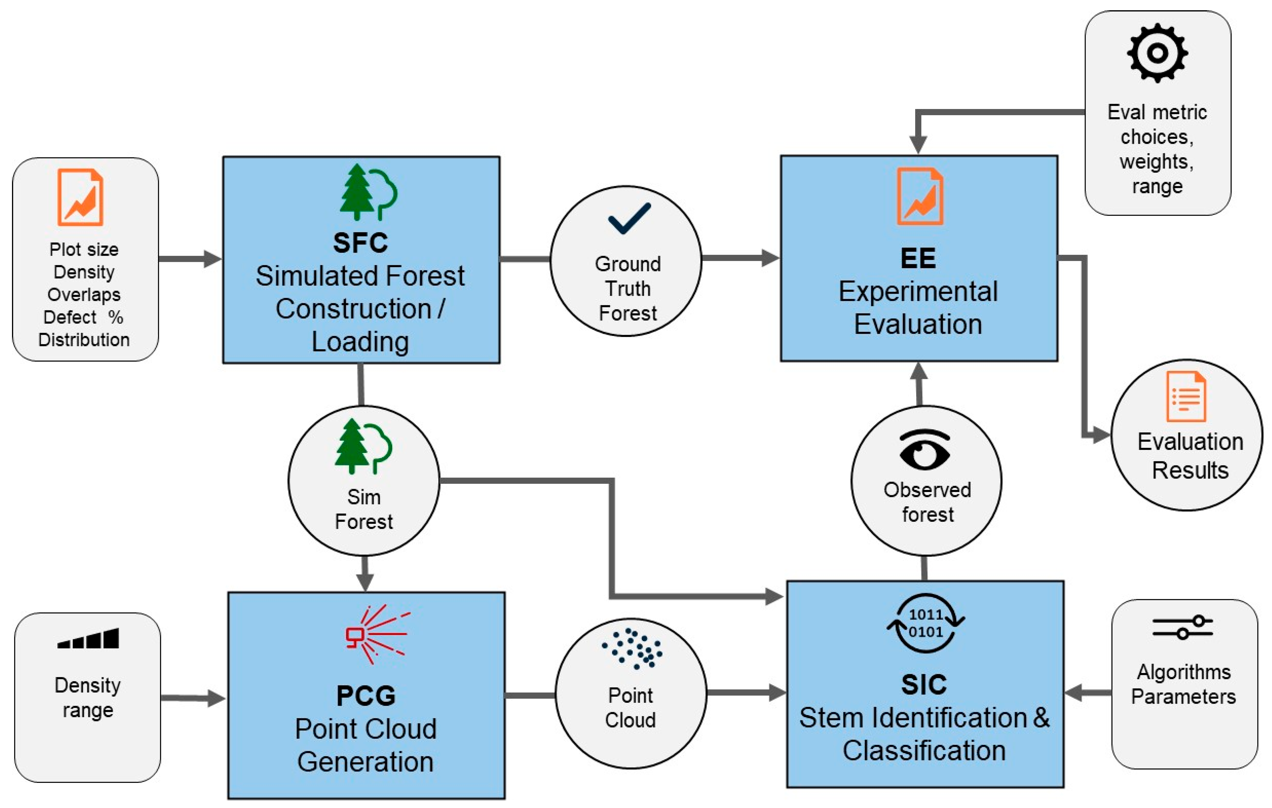
2. Materials and Methods

The TCF framework consists of four innovative primary components (Figure 2):

• Synthetic Forest Creation (SFC): This component enables the generation of synthetic forests with tunable attributes, such as forest size, tree density, overlap rates, and probabilities of tree defects.
• Point Cloud Generation (PCG): PCG allows for adjustable density and range in point cloud data, essential for accurately rendering tree structures within the simulated environment.
• Stem Identification and Classification (SIC): The SIC algorithm specialises in identifying and characterising various stem shapes, including hidden, bent, and curved trees, providing a realistic representation of the complex structure found in natural forests. Utilising point cloud data, the simulated forest structure closely aligns with the format used by real-world Ponsse harvesters [7].
• Experimental Evaluation (EE): This module provides a new set of metrics and statistical tools to validate simulation outcomes, focusing on how closely point-cloud-derived data matches the ground truth for each tree stem.

This paper proposes an initial set of experiments within the TCF framework, designed to be sensitive to critical parameters influencing the quality of the SIC process. A pivotal aspect of step EE involves defining precise evaluation metrics to assess the SIC’s performance effectively.

2.1. Used Tools

This framework aims to address the growing need for precision, efficiency, and adaptability in forest operations, enabling the next generation of harvesters to assist the operator seamlessly in diverse and complex environments. To achieve this, we leverage standard software tools and components, ensuring the framework is both robust and interoperable with existing technologies. By utilising widely adopted tools, we also facilitate scalability, flexibility, and ease of integration with the algorithms and hardware systems being developed. This approach allows the TCF framework to serve as a reliable test bed for innovations in harvester technology, ultimately accelerating their path to practical implementation.

Table 1. A list of tools and software used in the study.

Name	Version	Owner
Windows 10 Enterprise	22H2 (64-bit)	Microsoft Corporation, Redmond, WA, USA
Blender	3.6	Open-source
CloudCompare	2.11.3 (Anoia)	Open-source
Python	3.7	Open-source
numpy library	1.21.5	Open-source
Open3d library	0.17.0	Open-source
sklearn	1.0.2	Open-source

presents the tools and software used in our simulation. Windows serves as the operating system, hosting all operations and supporting the execution of essential software tools. In turn, Blender [17] was utilised for creating forest and tree stem models, as well as generating point clouds. Python version 3.7 was employed as the interpreted programming language for manipulating 3D models, generating point clouds, and conducting point cloud processing and analysis. CloudCompare version 2.11.3 (Anoia) [18] was used to examine the Point Cloud file prior to subjecting it to algorithmic analysis.

2.2. Synthetic Forest Creation SFC

In developing our simulation, several features were identified as critical to accurately replicating forest operations, each serving a distinct purpose to enhance realism. The forest size, for example, defines the scope of the simulation environment. Larger forests, such as those extending up to 50 hectares or more, are essential for simulating diverse scenarios like thinning, clear-cutting, and selective harvesting, while also allowing for the coordination of multiple machines. For our specific use case, we utilised a 1-hectare forest, striking a balance between manageability and operational complexity.

Equally important is the simulation of forest ground and terrain, which models the challenges of navigating different surfaces, including slopes and obstacles. Realistic terrain is vital for testing machine stability, manoeuvrability, and fuel efficiency across conditions such as flat, rolling, and rugged landscapes. In our case, we focused on flat and rolling terrain, simulating varied ground conditions without excessive complexity. To simulate rolling terrain, Blender’s Displace Modifier was employed to deform a subdivided plane using procedural textures, effectively capturing the irregularities found in natural landscapes. The process began with the addition of a mesh plane, which was then appropriately scaled and subdivided to increase its mesh density. This subdivision ensured sufficient geometry for detailed displacement. A Displace Modifier was applied via the Modifiers panel, and a new texture was created using procedural types such as Clouds or Musgrave, both well-suited for generating organic surface variation. Finally, the Strength and Midlevel parameters of the modifier were adjusted to fine-tune the elevation intensity and baseline, resulting in a realistically undulating terrain surface [17,19]. The number of tree stems, another essential feature, directly influences machine productivity and cutting strategies. A higher density of trees can complicate manoeuvring and impact the efficiency of harvesting operations. In our simulations, we utilised forest stands characterised by stem densities of 10, 24, 192, 550, and 1100 tree stems per simulated forest. These stem counts were selected to represent a gradient of forest densities, ranging from sparse to dense. Drawing on insights from Lang [20] and Forest Europe [21], the density of 550 stems per forest was identified as the primary configuration for our simulations. Based on NHS Forest [22], Bertault et al. [23], Kärhä and Keskinen [24], and Webber [25], 1100 was the recommended stem count per hectare across different forest types, management practices, and geographical locations. Therefore, we simulated a forest with 1100 stems, serving as the representative baseline for denser forest conditions. The lower stem counts were incorporated to establish an incremental progression in the simulation setup, enabling us to systematically evaluate the environment’s impact on algorithm performance and ensure robustness across varying forest densities. This approach allowed for the gradual refinement of both the simulation environment and the algorithm under test. Similarly, the spatial arrangement of tree stems, whether random or grid-like, determines how harvester operators navigate and position machines for selective harvesting. We tested both even and uneven stem distributions to vary the difficulty and realism of the tasks.

The height of tree stems plays a pivotal role in shaping machine reach, cutting removal strategies, and log sorting. Our simulations incorporated a range of tree heights, from 11 to 27 m, to reflect the diversity found in natural forests. In conjunction with height, stem distribution and shape also contribute to the complexity of harvesting. Irregular tree shapes, for instance, pose unique challenges during felling and piling logs cut, and we opted to use irregular forms to simulate curved objects for our use cases.

In terms of stem diameters, variations are necessary in order to simulate different log sizes and their associated challenges, from saplings with small diameters to larger sawlogs. For our purposes, we maintained a relatively fixed diameter to focus on other factors like tree stem shape. Similarly, tree stem orientation, whether leaning or upright, affects machine positioning and cutting angles, although we did not incorporate this feature in our simulations, leaving all stems in an upright position. Ground-truth measurements, obtained via Python scripts, provide a method for validating the accuracy of simulated data by comparing it with ground-truth measurements of height, diameter, volume, and position. These precise measurements are crucial for machine-learning applications, research, and the optimisation of harvesting algorithms. Lastly, the conversion of 3D models into point clouds enhances spatial data analysis and supports integration with real-world LiDAR scans. For our use case, we used point cloud data in the (.pcd) format, enabling detailed visualisation and advanced analysis of forest environments, with adjustable point densities to suit various simulation requirements.

Together, these features form a comprehensive framework that allows for realistic forest characteristics. To visualise and analyse forest structures, we constructed a simulated forest environment using Blender version 3.6, an open-source 3D modelling software. The simulated forest spans an area ranging from 0.02 to 1 hectare, meticulously designed to replicate the natural variability in tree growth and spatial distribution. This model incorporates a diverse array of tree stems, capturing the complexity inherent in natural forests.

To generate 3D tree stems, the Sapling Tree Gen add-on—available by default in Blender—was used. Some stems were created with perfectly straight growth, while others incorporated predefined curves to reflect natural morphological variations influenced by environmental factors. Afterwards, the tree stem models were converted into mesh objects using the built-in Blender feature. These mesh models were then duplicated to produce the desired number of stems using a Python script executed within Blender’s scripting interface.

This diversity in stem architecture enables a comprehensive investigation into the interplay between tree form and both the structural and visual characteristics of the forest. Moreover, it facilitates the evaluation of tree detection accuracy under varying morphological conditions. The spatial arrangement of trees within the simulation further enhances its analytical potential. Tree stems are distributed in both uniform and heterogeneous patterns, allowing for comparative analyses between managed forests, characterised by orderly planting and naturally occurring stands with irregular spacing.

By incorporating variations in both tree structure and spatial organisation, this simulated forest serves as a versatile framework for ecological research, visual landscape assessments, and spatial modelling applications. This approach to simulated forest construction provides a controllable, replicable environment that aids in studying the impacts of forest density, tree form, and spatial patterns without the complexities of fieldwork. Through this model, we aimed to balance realistic representation and research adaptability, enabling a detailed examination of forest dynamics in a virtual setting. Figure 3 illustrates the forest plot sizes, the number of tree stems, and the forest terrain used with this simulation.

Forests I–X in Figure 3 visualise simulation scenarios constructed for the initial evaluation of the simulation platform.

Table 2. Simulated forest parameters setup.

Forest ID	Size (In Meters)	Number of Stems	Distribution	Tree Stem Shape	Terrain
I	10 × 20	10	Even	Curved and one straight	Most rolling
II	20 × 40	24	Uneven	Straight and curved	Predominantly flat
III	20 × 40	192	Even	Straight and curved	Predominantly flat
IV	20 × 40	192	Uneven	Straight and curved	Rolling
V	100 × 100	550	Even	Straight and curved	Rolling/flat
VI	100 × 100	550	Uneven	Straight and curved	Rolling/flat
VII	100 × 100	550	Evenly/clusters	Straight and curved	Rolling/flat
VIII	100 × 100	550	Uneven/clusters	Straight and curved	Rolling/flat
IX	100 × 100	1100	Even	Straight and curved	Rolling/flat
X	100 × 100	1100	Uneven	Straight and curved	Rolling/flat

summarises the main parameters of these forests. Plot sizes, the number of tree stems, and terrain shapes utilised in the simulation are given: (I) a 10 m × 20 m (meters) plot (0.02 hectares) on uneven terrain, featuring nine curved tree stems and one straight tree stem; (II) a 20 m × 40 m plot (0.08 hectares) with 24 uniformly distributed straight and curved stems on flat terrain; (III) a 20 m × 40 m denser plot with 192 uniformly distributed straight and curved stems on flat terrain; (IV) a similar plot to Forest III with uneven stem distribution; (V, VI, VII, VIII) 100 m × 100 m plots (1 hectare) with 550 stems; and (IX, X) 1100 stems, distributed evenly, unevenly, or in clusters.

2.3. Point Cloud Generation PCG

2.3.1. Simulating Point Clouds

Simulating point clouds within a forestry simulation framework fulfils several important purposes, such as generating synthetic datasets to test algorithms and accurately modelling the structural components of trees, including stems, branches, and foliage. The choice of shooting densities is crucial and depends on factors like the desired simulation detail, the scale of the forest being modelled, and the specific analyses to be performed.

Tree structure analysis involves replicating the spatial arrangement of tree components, while LiDAR data validation ensures that algorithms perform reliably on both synthetic and real-world datasets. The density of simulated point clouds must align with the intended level of detail, balancing accuracy with computational feasibility. Higher densities are indispensable for detailed, tree-level, or research-intensive applications, whereas lower densities are sufficient for broader, large-scale studies. This trade-off is a key consideration in ensuring that the framework meets its objectives efficiently. The selection of appropriate LiDAR point densities is crucial for ensuring that the data collected aligns with the specific requirements of different modelling scenarios. According to Watt et al. [26] and Swanson et al. [27], recommendations for LiDAR shooting densities vary depending on the desired level of detail and application. For large-scale mapping at the stand level, which often prioritises spatial coverage over fine-grain detail, a shooting density of 10 to 50 points per square meter is deemed sufficient. This resolution provides a broad overview of the terrain while maintaining efficiency in data acquisition. When the focus shifts to canopy modelling, where moderate detail is required to analyse tree structures and general foliage patterns, densities of 50 to 200 points per square meter become necessary. This increase allows for improved differentiation of canopy layers and better representation of vegetation dynamics. For scenarios demanding high-detail insights, such as species identification or biomass estimation, a significantly higher density range of 300 to 1000 points per square meter is recommended. This granularity ensures that smaller features are captured, enabling accurate species-level analyses and precise biomass calculations. Lastly, for ultra-detailed modelling aimed at capturing intricate structures like individual branches, densities exceeding 1000 points per square meter are essential. Such detailed resolutions enable comprehensive structural analyses and applications in areas like tree architecture modelling or precision forestry.

These recommendations underscore the importance of tailoring LiDAR data collection to meet the specific demands of each study, striking a balance between resolution and practicality for different ecological and forestry applications. Through our testing, we found that using 1000 points per tree stem provided the most accurate representation of the stem structure. Additionally, this density significantly improved the performance of algorithm testing, yielding more reliable and precise results. Converting the Blender simulated 3D tree stems to Point Cloud, we used the Python scripts inside the Blender environment and CloudCompare to visualise the generated point clouds. Figure 4 visualises the evenly and unevenly distributed tree stems in a point cloud format.

2.3.2. Integrating LiDAR Sensor and Point Cloud Generation

To simulate the LiDAR sensor within the Blender simulation environment, we selected the Ouster LiDAR OS0 64 (Ouster Inc., San Francisco, CA, USA) sensor, which was mimicked, and configured its parameters according to the specifications provided in the sensor’s datasheet [28]. However, certain adjustments were made for simplification purposes. For instance, the frame rate was set to 1 frame per second (fps) to streamline processing, despite prior testing at 10 fps, which yielded consistent results.

The sensor’s initial position, orientation, and height were carefully determined to align with its real-world placement on a harvester. Once activated, the LiDAR sensor, controlled by our Python script, begins scanning the virtual scene from its designated starting position, continuously capturing spatial data until it reaches its final destination. The total number of frames required for this process is computed based on the distance between the start and end positions, ensuring accurate simulation of the sensor’s movement at the defined speed and frame rate.

The point cloud data from each frame is stored as an individual file in binary PCD format. Additionally, the point clouds from each frame are appended to the (all_points) list by adding the elements of the frame_points list. This process ensures that all points captured in the current frame (frame_points) are continuously accumulated into a comprehensive dataset (all_points). This approach facilitates the aggregation of point cloud data across multiple frames, enabling a more complete and continuous representation of the scanned environment. The aggregated point cloud data (all_points) is then saved in binary PCD format, serving as the primary file for analysis and measurements. Figure 5 displays a point cloud from a single frame alongside point clouds from all captured frames. Figure 6 illustrates the generated point clouds using the CloudCompare tool, including both single-frame and multi-frame aggregated data on the synthetic forest. For more details on how the point cloud was generated, please refer to Appendix A.

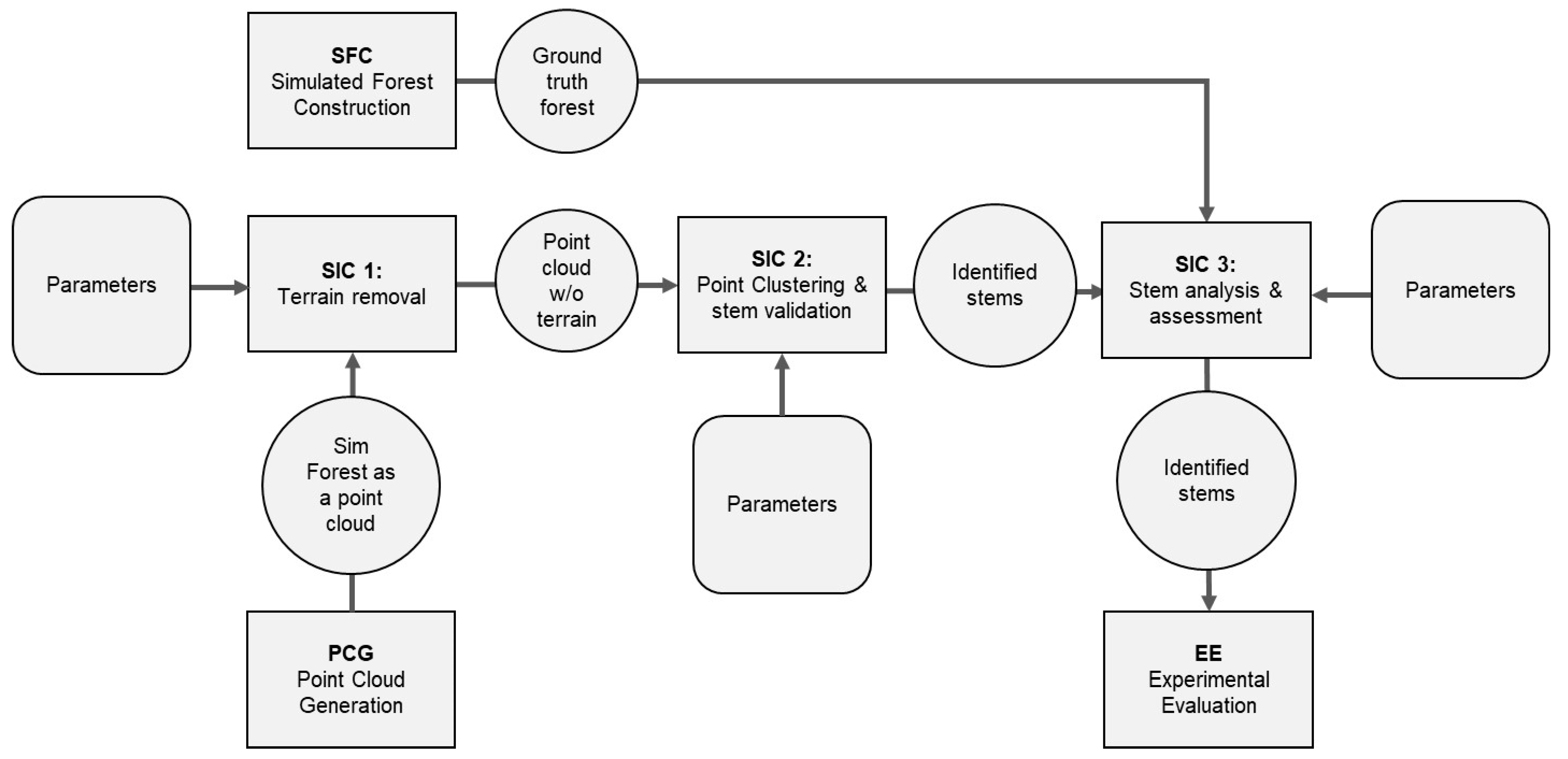
2.4. Stem Identification and Classification SIC

TCF is used to evaluate one stem identification and classification (SIC) algorithm at a time. The other TCF components specify the forest and technology environment in which the SIC algorithm is tested. The interfaces between the components and the algorithm are the virtual forest representation, from component PCG, and the ground-truth synthetic forest representation, from component SFC. The latter is either fully synthetic or based on a real forest. The output is a JSON format representation. The SIC algorithm comprises three steps, as illustrated in Figure 7.

Step 1: Ground (Terrain) Point Removal.

This step employs a grid-based approach to isolate above-ground vegetation from the terrain. The forest plot is divided into uniform grid cells of size 1 × 1 m (default). Within each cell, the point with the minimum z-coordinate is identified. All points at most 20 cm above this local minimum are classified as ground and subsequently removed. These parameters were selected based on typical terrain roughness observed in forested environments and are consistent with practices in related literature. In sensitivity tests, increasing the cell size above 2 m led to under-detection of micro-topographic variation, while reducing it below 0.5 m increased computational time with minimal accuracy gains. The output is a terrain-filtered point cloud containing primarily above-ground vegetation.

Step 2: Clustering and Stem (Tree) Validation.

Density-based clustering is used to group spatially coherent points likely representing individual trees. For nearest-neighbour search, we use a KD-Tree implementation from the scikit-learn Python library. Clustering is performed using a fixed-radius approach with a search radius of 0.3 m, based on average crown proximity in dense forest stands. Clusters are retained as potential trees if their height exceeds a minimum threshold of 2.5 m, calculated as the difference between maximum and minimum z-coordinates. These values were selected to exclude underbrush and low-lying vegetation. A parameter sweep showed that decreasing the height threshold below 2.0 m increased false positives (e.g., shrubs), while increasing it beyond 3.0 m led to omission of smaller trees.

The output is a set of validated tree clusters, each consisting of a group of points that meet the spatial and height criteria. These clusters serve as candidate trees for further structural analysis.

Step 3: Stem (Tree) Analysis and Assessment (Property Extraction).

For each tree cluster, key geometric attributes are extracted. The central position is computed as the mean of the x- and y-coordinates, and the height is derived from the maximum minus minimum z-values. These measurements are stored in a structured JSON format for reproducibility and further analysis. Figure 8 shows a 3D visualisation of the identified trees, with unique colour coding for each stem. As described in Algorithm 1, the stem data is processed and stored in the JSON format.

Algorithm 1 Pseudocode for processing stem data in the JSON format.

begin  set timestamp = "20250213_035113"  set total_objects_count = 24  for each object_id in total_objects_count do   create measured_object    id = object_id    name = "tree_" + object_id    h = MEASURE height    dbh = MEASURE (diameter at breast height)    maxcurve = CALCULATE max_curve    quality = 1 // default straight tree    cp = CALCULATE center_position = [x, y, z]    d = CALCULATE distance from scene center   store measured_object = (id, name, h, dbh, maxcurve, quality, cp, d)  end for end

Key features and advantages of the representation and the algorithm are adaptability, efficiency, and robustness:

• Adaptability: The algorithm can be tailored for diverse forest types through adjustable parameters, enabling it to handle varying tree sizes, densities, and point cloud characteristics.
• Efficiency: The grid-based ground filtering is computationally efficient, while the KD-tree structure accelerates point clustering.
• Robustness against noise: The algorithm effectively handles sparse noise and terrain irregularities by filtering off the ground points and applying minimum point thresholds.
• 3D visualisation capabilities: Enhance user experience in forest management and research.

Despite its strengths, the algorithm faces challenges in some simulation scenarios. Dense canopies, where tree crowns overlap, may obscure individual tree boundaries. Similarly, irregular tree shapes can complicate clustering, and small trees below the height threshold may go undetected. Addressing these limitations requires further refinement to ensure robust performance in complex forest environments.

In summary, this algorithm represents a powerful platform for tree detection and property calculation in forest simulations. It balances computational efficiency with adaptability to diverse scenarios while suggesting features for improvement.

2.5. Experimental Evaluation EE

2.5.1. Overview of Evaluation Metrics

The purpose of the TCF platform is to enable a systematic and controlled evaluation of forestry algorithms. The motivation for this stems from the need to test, refine, and validate emerging algorithms in a risk-free, cost-effective, and highly customisable setting before their deployment in real-world forestry operations. Traditional field testing presents significant challenges, including variability in environmental conditions, logistical constraints, and high operational costs. By leveraging a virtual simulation platform, researchers and developers can conduct repeatable experiments under standardised conditions, ensuring rigorous performance assessments across diverse scenarios.

Furthermore, this virtual framework fosters innovation by allowing rapid prototyping and iterative improvements of algorithms, facilitating a deeper understanding of complex forestry dynamics. It also enhances collaboration among interdisciplinary teams by providing a shared, data-rich environment where new methodologies can be explored, compared, and optimised. In essence, the platform serves as a bridge between theoretical algorithm design and practical implementation, accelerating advances in precision forestry and sustainable forest management practices.

To compare the ground-truth forest (synthetic forest) to the observed virtual forest, their representations matched. The forest matching and evaluation process is presented in Figure 9. The scores of the matches are aggregated for comparison of the forestry algorithms under development.

The TCF framework fosters systematic evaluation experiments structured by a range of independent and dependent variables. The dependent variables include the following:

• Total Matches: This will present the total number of matched tree stems, ground-truth vs. observed tree stems.
• Quality Error (%): The percentage of incorrectly classified tree stems.
• Quality Correct (%): The percentage of correctly classified tree stems.
• RMSE Quality: Root Mean Square Error of the matches quality.
• Correct Matches Quality: The count of correctly matched quality.
• Wrong Matches Quality: The count of incorrectly matched quality.
• Evaluation Score (%): Presents the accuracy of tree stem classification.

The independent variables include the following:

• LiDAR properties (including three different resolutions and maximum reach distance):

  ▪

  Resolution: The available resolutions with the selected LiDAR were 512, 1024, and 2048. Each resolution varies in levels of detail that can be observed.

  ▪

  Maximum reach distance: Defines the farthest point the LiDAR can detect objects. The selected LiDAR offer a longer distance reach, but we have limited it to 50 m.

• Forest properties:

  ▪

  Forest size (refer to Table 1).

  ▪

  Tree stem distribution (even, uneven, or clusters) by location and quality.

  ▪

  Tree stem characteristics (varying heights, straight vs. curved structures).

These allow assessing experimentally the impact of the properties of the LiDAR, the properties of the tree classification algorithm, and forest properties on the tree classification algorithm performance. To illustrate this, we carried out twelve sample experiments using the sample Forests I–X defined above. While the majority of dependent variables are fairly standard and self-explanatory, the Weighted Evaluation Credit (%) is specifically designed for forestry algorithm evaluation (Figure 10).

2.5.2. Weighted Classification Assessment

The standard evaluation metrics discussed above are binary: an observed tree either fully matches a ground-truth tree or does not match at all. However, practical evaluations may have multiple non-binary criteria like straightness, diameter, and length, to be satisfied at once. There may also be disjunctive criteria, e.g., tree_species = birch OR oak. Further, partial matching of the criteria may be partially rewarded in evaluation. This makes weighted classification an interesting scenario. We shall now develop an evaluation metric for multiple non-binary criteria. We call it wc (for weighted classification).

The properties of wc are as follows:

• It compares two forests, the ground-truth forest GTF, and the observed forest OF.
• Both forests have the same ground coordinate spaces and similar representations as sets of trees using JSON (see Algorithm 1).
• GTF is our “correct” forest representation, derived from the real world or fully synthetically constructed. OF is the result of the SIC component reflecting the performance of the SIC algorithm.
• wc takes one tree ot of OF at a time and searches for its NN gtt in GTF. For a match, the NN gtt must be within distance d from the position of ot. If there is no match within d, ot is classified as “not matched”. If there is a match, the pair (ot, gtt) is assessed for all criteria (e.g., “tree; straight”) and sent to scoring.
• Without loss of generality, this study focuses on the classification of a single property: the shape of trees, categorised as either Straight (S), Curved (C), or Other (X).
• The scoring parameters determine how much the SIC algorithm is credited for full or partial matching.
• The credits are summed for an overall score for the SIC algorithm under test.

Next, we define the function wc more formally using set-theoretic notation. We begin with preliminaries regarding data representation as objects and basic functions (Table 3).

Table 3. Basic notations.

Object	Explanation
Tuples	Data objects are represented by listing their attributes a1, a2, …, an as tuples t = (a1, a2, …, an). The attribute values of tuples are referred to by their positions; e.g., t [1] gives the first attribute of t. When attributes have names, e.g., an1, an2, …, ann, the attribute values can be referred to by the names; e.g., t (an) gives the value of the attribute of t named an.
Sets	Sets of data objects are represented by enumerating their elements e1, e2, …, en between braces as s = {e1, e2, …, en}. Set membership and non-membership are denoted as e ∈ s and e ∉ s, respectively.
Lists	Lists of data objects are represented by enumerating their elements e1, e2, …, en between angle brackets as s = <e1, e2, …, en>. We denote its head component and tailing list by <head|tail>. Adding one element e to list L is denoted by L ⊕ e (alternatively <L, <e>>).
Trees	Trees are represented as tuples: t = ⟨id, name, height, dbh, max_curve, quality, center_position (x, y, z), class, NNid). Among the attributes, id uniquely identifies the tree, (x, y, z) represents its coordinates, class shows its classification as Straight (S), Curved (C), and other (X) tree, and NNid records the identifier of the nearest neighbour when resolved (or is assigned N/A if no NN is found).
Forests	Forests are represented as sets of tuples: f = {t1, t2, …, tk}.
	Let OTi and GTij be two trees, GTF be a forest, and d be the max distance allocation. The Euclidean distance of OTi and GTi is denoted by dist(OTi, GTj). The nearest neighbour of OTi within GTF is as follows Equation (1): nn(OTi, GTF, d) =                                              (1)   case 1: GTi ∈ GTF,     if ∀ GTj ∈ GTF ⋏ i ≭ j:      dist(OTi, GTj) ≤ dist(OTi, GTj) ⋏      dist(OTi, GTj) ≤ d   case 2: “N/A”,      else

Table 3. Basic notations.

Object	Explanation
Tuples	Data objects are represented by listing their attributes a1, a2, …, an as tuples t = (a1, a2, …, an). The attribute values of tuples are referred to by their positions; e.g., t [1] gives the first attribute of t. When attributes have names, e.g., an1, an2, …, ann, the attribute values can be referred to by the names; e.g., t (an) gives the value of the attribute of t named an.
Sets	Sets of data objects are represented by enumerating their elements e1, e2, …, en between braces as s = {e1, e2, …, en}. Set membership and non-membership are denoted as e ∈ s and e ∉ s, respectively.
Lists	Lists of data objects are represented by enumerating their elements e1, e2, …, en between angle brackets as s = <e1, e2, …, en>. We denote its head component and tailing list by <head|tail>. Adding one element e to list L is denoted by L ⊕ e (alternatively <L, <e>>).
Trees	Trees are represented as tuples: t = ⟨id, name, height, dbh, max_curve, quality, center_position (x, y, z), class, NNid). Among the attributes, id uniquely identifies the tree, (x, y, z) represents its coordinates, class shows its classification as Straight (S), Curved (C), and other (X) tree, and NNid records the identifier of the nearest neighbour when resolved (or is assigned N/A if no NN is found).
Forests	Forests are represented as sets of tuples: f = {t1, t2, …, tk}.
	Let OTi and GTij be two trees, GTF be a forest, and d be the max distance allocation. The Euclidean distance of OTi and GTi is denoted by dist(OTi, GTj). The nearest neighbour of OTi within GTF is as follows Equation (1): nn(OTi, GTF, d) =                                              (1)   case 1: GTi ∈ GTF,     if ∀ GTj ∈ GTF ⋏ i ≭ j:      dist(OTi, GTj) ≤ dist(OTi, GTj) ⋏      dist(OTi, GTj) ≤ d   case 2: “N/A”,      else

Consider the sample tree object gtt1 = < 5, gttn1, 8.39, 0.28, (3.7, 8.5, 4.20), S, 4 >. This describes a ground truth tree with the follow properties:

• id = 5;
• name = gttn1;
• height = 8.39;
• dbh = 0.28;
• center_position(x, y, z) coordinates: 3.7, 8.5, 4.20;
• class = S (Straight);
• NNid Nearest Neighbour ID = 4. Initially, all NN id values (gtt[7] and ot[7]) are set to N/A.

Tree classification assigns classes to trees but does not give credit values to the assignments. This is achieved by representing all possible combinations of observed and ground-truth classes, giving them credit class labels, and quantifying the credit classes. The evaluation algorithm may then credit each case flexibly. As an example,

Table 4. Ground-truth trees vs. trees observed by SIC Classification. E indicates an exact match, A is an almost correct match, and N indicates presence in the ground truth but not in the observed forest.

Ground Truth Classification	Observed by SIC Classification
	Curved (C)	Straight (S)	Other (X)
Curved (C)	E	A	N
Straight (S)	A	E	N
Other (X)	N	N	-

shows the possible classifications of proposed (gtt, ot) pairs when the three classes S, C, and X are considered. In Table 4, ‘E’ indicates an exact match, ‘A’ indicates an almost correct match, and ‘N’ indicates that the item was present in the ground truth but was of an uninteresting type or had no match in the observed forest.

The weighting of each matching case E, A, and N can now be given as a tuple Credit = ((E, w1), (A, w2), (N, w3)). For example, Credit1 = ((E, 2), (A, 1), (N, 0)) gives credit class E twice as much credit compared to A-classification, and N-class gives no credit.

The evaluation framework allows flexible setting of the number of classes and their weights. With no loss of generality, we use positive integers as weights in the examples of the present paper. The requirement is that the classes are mutually exclusive, i.e., no tree can belong to more than one class, that the scores are positive integers, and that no observed tree is assigned as the NN for more than one ground-truth tree. A more in-depth exploration of alternative scoring mechanisms is left for future studies.

The basic matching of a gt tree and its candidate NN in OF, ot, is recorded by assigning the pair (gtt, ot) a credit score. The assessment of the classification of entire forests happens by aggregating the assigned elementary scores. The latter is given by the function quant (Equation (2)):

quant(gtClass, otClass, CaseTable, Credit) = Credit[CaseTable(_{gtClass, otClass})]

(2)

where gtClass and otClass are the ground-truth and observed classes, respectively (∈ {C, S, X}), and used to index CaseTable (e.g., Table 4), which provides classification mappings to credit cases, and Credit (e.g., Credit1 above), which determines the scoring of each classification outcome. The result (gtClass, otClass, Credit) is appended to the list EL.

We collect the evaluation scores of tree pairs by the function em defined next. The goal is to evaluate the classification performance by constructing an Evaluation Matrix (EM), which accumulates weighted classification results.

Function arguments are as follows:

• The set of tree classes: C = {S, C, X};
• Ground truth classification: gtClass ∈ C;
• Observed classification: otClass ∈ C;
• Classification CaseTable: C x C → {E, A, N}, mapping pairs of observed and true classes to evaluation cases;
• Credit function assigning weights to classification cases: Credit: {E, A, N} → I⁺;
• Evaluation List (EL) is a list of credit tuples (gtClass, otClass, Credit), one for each matched pair of trees.

The evaluation matrix EM cumulates the credit data. It is initialised as a zero matrix of dimensions |C| X |C| by setting EM: EM[i, j] = 0, when 1 ≤ i, j ≤ |C|.

Then, it is filled on the basis of the list EL = < e | EL’ > credit tuples. The addition of one credit tuple (gtClass, otClass, Credit) to EM cell EM[gtClass, otClass] is denoted as

EM ⊕ < gtClass, otClass, Credit >

which yields a modified matrix EM’, with cell EM’[gtClass, otClass] = EM[gtClass, otClass] + Credit. As a function, the cumulation of the credits is given by the function $em$ (Equation (3)):

em(EM, << gtClass, otClass, Credit > | EL’ >) =   
case 1: em(EM ⊕ < gtClass, otClass, Credit >, EL’),
if |EL| > 0            
case 2: EM,                  
otherwise.            

(3)

Credit calculation for an entire forest sums the credits accumulated in EM. This is calculated by the function wc. The argument is the evaluation matrix EM. The function wc calculates the entire credit for correctly classified observed trees by summing up the diagonal cells in EM using the function wcnume (Equation (4)):

wcnume(EM) = Σ_c=1…dim EM[c, c],

(4)

where dim is the dimension of the matrix. Then, it calculates the sum of all cells in EM using the function wcdeno (Equation (5)):

wcdeno(EM) = Σ_I,j…dim EM[i, j],

(5)

where dim is the dimension of the matrix. As the final step, wc calculates the proportion of correctly classified observed trees as a percentage 0% … 100% (Equation (6)):

wc(EM) = 100 × wcnume(EM)/wcdeno(EM)

(6)

The properties of the function wc are as follows:

• A higher credit percentage indicates better classification performance, where observed classes match ground-truth classification with high credit values.
• The function accounts for misclassifications by distributing credits across different matrix entries.
• The case table mappings and credit function allow for flexible weighting and, thus, adapting the method to different classification criteria.

This formulation provides a systematic approach to evaluating classification accuracy using a structured credit matrix. The following section provides several examples on the use of the function wc and the entire evaluation process.

3. Simulation Results

This section presents the results of each simulated forest, as detailed in Section 2.2. The ‘550 stems per hectare’ scenario was selected as a representative example, as it lies near the midpoint of the tested density range (10–1100 stems/ha) and features a relatively even distribution of Forest V and a more uneven distribution of Forest VI. Although the approach is applicable across all defined forest types, this case effectively demonstrates the typical spatial patterns and predictive performance of the TCF framework. We analysed five evaluation experiments:

• Experiment 1: Mapping the positions of the ground-truth and observed stems and quality heatmap without the LiDAR integration;
• Experiment 2: LiDAR resolution effect in an evenly populated forest;
• Experiment 3: LiDAR resolution effect in an unevenly populated forest;
• Experiment 4: Stem quality evaluation for all defined Forests I–X;
• Experiment 5: Weighting the credits.

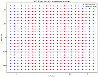
Experiment 1: Mapping the positions of the ground-truth and observed stems and the quality heatmap without the LiDAR integration:

The visualisations presented in

Table 5. Sample heatmaps for Forests V and VI where each tree stem is represented by 1000 points without using a LiDAR sensor. S stands for straight, C for curved, and N for no match tree stems.

Forest	Matched	Quality Heatmap
V
VI

provide insights into tree stem matching and classification quality. In the matched column, the red dots represent the observed tree stems, while the blue dots indicate the ground-truth tree stems.

The quality heatmap illustrates the accuracy of tree stem classification. It is a direct derivation from the EM matrix defined above. It categorises matches based on tree shape:

• S:S (Straight) and C:C (Curved)—Correctly quality-matched tree stems;
• S:C or C:S—Misclassified stems, where a straight tree was observed as curved or vice versa;
• N:N—Missing tree stems, meaning they were neither observed nor classified, should always yield 0 credit;
• N:S or N:C—Tree stems present in the ground truth but missing in the observed data.

These tables help gain an overview and evaluate the accuracy of tree stem detection and classification under different conditions. For example, in Table 5, the higher layover of blue dots by red dots suggests a higher correct matching rate for the observed tree stems. This is confirmed by the quality heatmap, which shows higher numbers and different colour codes for Forest V.

A confusion matrix summary between the V and VI Forest matches is presented in

Table 6. Confusion matrix summary between the V and VI Forests matches.

Metric	Forest V (Even)	Forest VI (Uneven)
Correct Classifications	90.9% (500/550)	74.4% (409/550)
Misclassifications	9.1% (50/550)	13.1% (72/550)
Missed Trees (N Category)	0% (0/550)	12.5% (69/550)

. The classification algorithm performed better in Forest V than VI, with a higher accuracy (90.9% vs. 74.4%), fewer misclassifications (9.1% vs. 13.1%), and no missed trees (0% vs. 12.5%). It appears that the uneven distribution of tree stems presents a challenge to stem classification.

Experiment 2: LiDAR resolution effect in an evenly populated forest:

Table 7. Matching layout and quality heatmaps for evenly distributed Forest V at three different resolutions: lowest (512 points m^–2), medium (1024 points m^–2), and highest (2048 points m^–2).

Resolution	Matched	Quality Heatmap
512
1024
2048

and

Table 8. The matching layout and quality heatmaps for the selected test Forest VI at three different resolutions: lowest (512 points m^–2), medium (1024 points m^–2), and highest (2048 points m^–2).

Resolution	Matched	Quality Heatmap
512
1024
2048

display the results obtained after integrating the LiDAR sensor and generating the measured point clouds. In these simulations, the LiDAR sensor is configured with the following parameters: an initial position of (X, Y, Z) = (0, −50, 2) and a final position of (0, 50, 2), moving along the Y-axis while scanning the forest. From the “Matched” column, it is evident that the scans do not capture the entire simulated forest. This is expected, as the sensor’s maximum range is limited to 50 m, and there are occlusion and sensor resolution limitations. In a real-world scenario, the harvester moves during thinning operations, allowing previously unreached trees to be scanned. As a result, there is a noticeable drop in the number of matched ground-truth tree stems compared to observed trees since fewer observations are recorded than the actual number of trees. This reduction directly impacts the accuracy of tree stem quality classification. Additionally, the sensor’s height from the ground, set at 2 m, influences tree stem height measurements. When the sensor is positioned very close to a tree, it may not capture the full stem, leading to inaccuracies. This, in turn, affects other tree property measurements, such as the diameter at breast height (DBH) and curvature values. From the quality heatmap column, it is evident that a higher LiDAR resolution improves tree stem matching and enhances tree stem quality classification in these scenarios. The values within the heatmaps were assigned as follows: S = 1, C = 1, and N = 1 as weight/credit. The colour codes used here are primarily for visualising the highest values and their corresponding classes.

Table 7 displays heatmaps of the evenly distributed Forest V at varying resolutions, illustrating a clear trend: as the resolution increases, so does the precision in detecting and mapping tree stems. This enhanced resolution not only improves the stem coverage but also refines the accuracy of tree stem quality classification. The progression is evident at lower resolutions, where tree stems appear fragmented or partially obscured, whereas, at higher resolutions, their structure becomes more distinct, enabling more reliable evaluations. This finding underscores the critical role of the resolution in advancing forest monitoring and ecological studies.

Experiment 3: LiDAR resolution effect in an unevenly populated forest:

Table 8 presents heatmaps of the unevenly distributed Forest VI at varying resolutions, revealing a pattern similar to that observed in Forest V: higher resolutions enhance the precision of tree stem detection and mapping. However, an exception emerges at the lowest resolution, where the algorithm identifies a tree stem in the observed data that is absent in the ground truth. This discrepancy results in a total stem count of 551 instead of the expected 550 in the quality classification. This deviation can be attributed to the uneven spatial distribution of tree stems, which introduces occlusion effects where some trees become obscured behind others, limiting the sensor’s ability to detect all stems as effectively as in a more evenly distributed forest.

Experiment 4: Stem quality evaluation for all defined Forests I–X:

Table 9. Summary of the tree stem quality (straight and curved) and the total matched evaluation experiments performed based on 1000 points stem^–1. The minimum and maximum performance values are highlighted in bold and italics, respectively.

Forest ID 1	Features 2	Quality Error (%) 3	RMSE Quality 4	Total Matches 5	Quality Correct (%) 6	Evaluation Score (%) 7	Correct Matches Quality 8	Wrong Matches Quality 9
V	1000 stem–1	9.1	0.30	550	90.9	92.8	500	50
VI		12.3	0.35	481	74.0	75.2	422	59

¹ The Forest ID column contains the simulated Forest number/ID. ² The Features column represents the number of points per stem. ³ The Quality Error (%) column quantifies the percentage of misclassified tree stem quality, distinguishing between straight and curved stems. ⁴ The RMSE Quality column provides the root mean square error (RMSE) associated with tree stem quality classification accuracy. ⁵ The Total Matches column represents the total number of matches identified when comparing ground truth data with point cloud data. ⁶ The Quality Correct (%) column contains the percentage of the correctly matched quality. ⁷ The Evaluation Score (%) column presents the results of the quantification process, derived from a predefined calculation matrix, where values were assigned as follows: S = 2, C = 1, and N = 1. ⁸ The Correct Matches Quality column contains the count of the correctly matched quality. ⁹ The Wrong Matches Quality (%) column contains the count of the wrongly matched quality.

summarises the tree stem quality evaluation for two different forest conditions (V and VI) based on 1000 points per stem. The key metrics include quality error, RMSE quality, total matches, quality correctness, evaluation score, and the number of correct and incorrect quality matches.

• The tree stem classification algorithm performed better in Forest V than in Forest VI across all metrics, indicating better tree stem quality classification and matching accuracy.
• Quality Error: Forest V has a lower error compared to Forest VI, meaning its quality assessment is more reliable.
• RMSE Quality: A lower RMSE in Forest V suggests a more precise quality estimation.
• Total Matches: More tree stems were successfully matched in Forest V, further supporting a better detection and classification performance.
• Quality Correctness: A higher percentage of correctly classified tree stems is observed in Forest V, highlighting the impact of forest conditions on classification accuracy.
• Evaluation Score: The overall evaluation score follows the same trend, with Forest V achieving a higher score, reinforcing its accuracy and reliability.
• Correct vs. Wrong Quality Matches: Forest V has more correct matches and fewer incorrect ones compared to Forest VI, indicating that errors are more frequent in the latter.

The results indicate that the tree stem quality evaluation performs better in Forest V than in Forest VI. The higher accuracy, lower error rates, and greater number of correct matches suggest that the conditions in Forest V are more favourable for precise tree stem quality classification.

Table 10. Summary of tree stem quality (straight and curved) and total matched evaluation experiments conducted using the LiDAR sensor. The minimum and maximum performance values highlighted in bold and italics, respectively, in each block.

Forest ID	Resolution 1	Quality Error (%)	RMSE Quality	Total Matches	Quality Correct (%)	Evaluation Score (%)	Correct Matches Quality	Wrong Matches Quality
I	512	30.0	0.55	10	70.0	63.6	7	3
	1024	30.0	0.55	10	70.0	63.6	7	3
	2048	40.0	0.63	10	60.0	54.5	6	4
II	512	25.0	0.50	24	75.0	74.1	18	6
	1024	16.6	0.41	24	83.3	83.8	20	4
	2048	20.8	0.46	24	79.2	77.4	19	5
III	512	22.4	0.47	174	77.5	72.0	135	39
	1024	24.7	0.50	166	73.3	69.1	125	41
	2048	24.2	0.49	161	75.7	68.0	122	39
IV	512	16.5	0.41	121	45.3	48.2	101	20
	1024	16.1	0.40	118	43.7	46.9	99	19
	2048	12.5	0.35	112	43.7	47.1	98	14
V	512	12.2	0.35	368	58.7	64.9	323	45
	1024	12.0	0.35	425	68.0	72.6	374	51
	2048	13.3	0.36	444	70.0	75.0	385	59
VI	512	17.2	0.42	313	82.7	48.7	259	54
	1024	11.8	0.34	347	88.1	56.6	306	41
	2048	13.2	0.36	370	86.7	59.7	321	49
VII	512	13.7	0.37	453	42.1	48.0	391	62
	1024	15.4	0.39	526	47.3	53.6	445	81
	2048	11.5	0.34	537	50.2	56.7	475	62
VIII	512	20.2	0.45	227	27.3	30.6	181	46
	1024	19.6	0.44	250	30.9	34.9	201	49
	2048	15.6	0.39	250	32.7	37.1	211	39
IX	512	16.5	0.41	544	83.4	47.9	454	90
	1024	14.1	0.38	671	85.8	58.4	576	95
	2048	13.2	0.36	772	86.7	66.0	670	102
X	512	19.8	0.45	449	80.1	34.3	360	89
	1024	17.0	0.41	553	80.3	43.5	459	94
	2048	35.1	0.45	614	80.1	46.7	492	122

¹ The Resolution column represents the LiDAR horizontal resolutions, where three distinct resolutions have been simulated based on the specifications of the selected LiDAR sensor.

presents a summary of the tree stem quality evaluation based on LiDAR sensor data across different simulated forests and resolutions. The evaluation includes quality error, RMSE quality, total matches, quality correctness, evaluation score, and the number of correct and incorrect quality matches. The analysis of Table 10 is as follows:

• Impact of LiDAR Resolution on Tree Stem Quality

  ▪

  Higher resolutions (1024 or 2048) generally improve accuracy in tree stem classification;

  ▪

  Lower resolutions (512) tend to have a higher quality error and lower quality correctness across most forests;

  ▪

  The RMSE quality decreases slightly with a higher resolution, suggesting better precision.

• Tree Stem Matching Trends

  ▪

  The total number of matches increases with a higher resolution, indicating that higher-resolution scans detect more tree stems;

  ▪

  Correct matches improve with the resolution, meaning that higher detail levels allow better tree classification.

  ▪

  Wrong matches tend to decrease at higher resolutions, though variations exist across forests.

• Forest-Specific Observations

  ▪

  Forests IX and X (largest datasets, 1100 trees ha–1) show a significant improvement in evaluation scores and quality correctness at higher resolutions.

  ▪

  Smaller Forests (I and II, fewer than 50 trees ha–1) show more variability in correct matches and evaluation scores.

  ▪

  Forests III–VIII exhibit gradual improvements in quality correctness with resolution, but at different rates.

• Trade-offs in LiDAR Scanning

  ▪

  While a higher resolution improves accuracy, it also increases the data processing requirements.

  ▪

  The improvement in evaluation scores and correct matches is not always linear across all forests.

  ▪

  Some forests, like Forest V, show only a slight increase in quality correctness despite the higher resolution, suggesting other factors, for instance, tree distribution, may influence accuracy.

In assessing the LiDAR-based tree stem classification across varying forest conditions, distinct patterns emerge. In small Forests (10–24 stems) with even or uneven distributions, the highest evaluation scores (63.6%–83.8%) and lowest quality errors (16.6%–30.0%) were observed at the 1024 and 512 resolutions, with the performance declining at the 2048 resolution, particularly in rolling terrains. As the stem density increased to 192, the evaluation scores diverged between evenly and unevenly distributed forests. Even distributions in predominantly flat terrains yielded a higher accuracy (72.0% at 512 resolution), whereas uneven forests in rolling terrains exhibited a lower performance (47.1% at 2048 resolution), suggesting terrain-induced complexities in detection. In large-scale forests (550–1100 stems), the highest evaluation scores (75.0% at the 2048 resolution) were recorded in evenly distributed stands, while clustered and unevenly distributed forests exhibited a lower accuracy (34.9%–46.7%), indicating that structural complexity hinders precise stem matching. Notably, the 2048 resolution consistently produced superior results in large forests, while the 512 resolution led to higher errors and reduced accuracy across all forest types. These findings underscore the influence of tree distribution, terrain, and resolution on LiDAR performance, highlighting the need for resolution optimisation in complex forest structures.

The results indicate that using higher LiDAR resolutions improves tree stem quality classification by reducing errors, increasing correct matches, and enhancing overall evaluation scores. However, not all forests benefit equally from higher resolutions, suggesting that factors such as tree density, terrain, or sensor limitations may also influence accuracy.

Experiment 5: Weighting the credits:

Table 11. Sample example of EM matrix heatmap of Forest I with a resolution of 512 point m^–2.

Weight/Credit	EM Matrix	Credit (%)
1,1,1		70.0
2,1,1		63.6
1,2,1		73.7

is an example of an Evaluation Matrix (EM) heatmap generated using different quantification weights/credits. In this scenario, classifications were weighted following the coding scheme W:x-y-z. This would present a comparative visualisation of EM heatmaps under different weighting schemes, demonstrating how different weight assignments influence the credit percentage. The heatmaps illustrate the observed versus ground-truth classifications for three different weighting scenarios, (1,1,1), (2,1,1), and (1,2,1), where the weights correspond to the categories S, C, and N, respectively.

The first heatmap (1,1,1) represents an equal weight distribution, yielding a credit percentage of 70.0%. The second heatmap (2,1,1) increases the weight for category S, leading to a lower credit percentage of 63.6%, suggesting that the weighting adjustment affects the overall classification performance. The third heatmap (1,2,1) assigns a higher weight to category C, resulting in the highest credit percentage of 73.7%. The colour gradient in the heatmaps visually represents the intensity of the observed correct classifications, with darker shades indicating higher correct classification frequencies. These results indicate that weighting adjustments significantly impact the evaluation metrics, highlighting the need for the careful selection of weight parameters when assessing the classification accuracy in different scenarios.

4. Discussion

Advancements in forestry automation, particularly in harvester technology, rely heavily on accurate tree stem detection using LiDAR sensors. However, evaluating the performance of LiDAR-based detection methods in real-world conditions presents significant challenges due to environmental variability and data collection constraints. The goal of the present paper was to establish a simulation framework for evaluating LiDAR-based tree stem detection in forestry applications, particularly with relevance to harvester technology development. By creating a controlled yet realistic simulation environment, we aimed to assess how well LiDAR-generated point clouds can represent and measure tree stems in comparison to their ground-truth geometry. The study sought to bridge the gap between virtual forest modelling and real-world harvester sensing, providing a platform for future research and algorithmic improvements. To address the overall research questions, we structured our approach as follows:

RQ: How can a valid and efficient simulation framework (TCF) be designed to support the development and evaluation of tree stem detection methods relevant to harvester technology?

The reliable detection and measurement of tree stems, especially those with natural curvature, remain a key challenge in forestry automation. Our TCF framework was developed to explore and validate an efficient approach to this problem. By integrating 3D-mesh-based tree models, LiDAR simulation, and automated point cloud processing, we created a pipeline that closely replicates real-world harvester sensing conditions. The results demonstrated that simulation-based methods can provide valuable insights into stem detection before field deployment, reducing costs and enhancing algorithm robustness.

To establish validity, we compared our simulation output with real LiDAR scans, ensuring similar statistical characteristics such as density and curvature representation. We also validated stem detection against known 3D models, measured curvature estimation errors, and sought expert assessments to confirm biological accuracy. Cross-validation with established LiDAR-based detection methods would further strengthen our findings; however, this is left for future research.

Efficiency was assessed by measuring the computational performance, including processing time, memory usage, and scalability across different dataset sizes. Additionally, the simulation framework minimises costly field tests by allowing algorithm refinement in a controlled environment. Lastly, we evaluated automation and robustness under varying conditions, tree heights, and tree densities to ensure adaptability in diverse forestry scenarios. We acknowledge that the noise levels in the generated LiDAR sensor data and handmade point clouds were minimal. A more in-depth analysis of these noise levels and their impact is left for future research.

Sub-RQ 1: What properties must a simulated forest environment possess to effectively represent real-world conditions for harvester algorithm development?

For the simulation to be representative, the virtual forests needed to capture the key characteristics influencing LiDAR perception, including the tree density, stem curvature, and occlusion effects. We designed ten distinct Forest scenarios, each incorporating different levels of tree spacing, orientation, and bending variations. This diversity allowed us to evaluate how environmental factors impact LiDAR performance. The results highlighted that occlusion plays a significant role in point cloud completeness and that tree density influences the accuracy of extracted stem properties. Based on our earlier study [12], stem curvature was identified as the most important property for this research.

Sub-RQ 2: How can the process of point cloud generation be realistically replicated within the simulation framework?

The process of simulating point cloud generation was designed to reflect realistic LiDAR sensor behaviour as used in harvesters. We configured the sensor’s height, angle, and resolution to align with potential real-world setups. The use of three different horizontal resolutions allowed us to analyse how varying data densities affect stem reconstruction. Our simulation results indicated that higher resolutions may affect the stem detection accuracy but come with increased computational costs. The Windows PC (see Table 1) was adequate for generating small and medium point clouds in this research. However, it experiences significant slowdowns when generating large point clouds, particularly during LiDAR sensor integration and when the number of frames is increased. This trade-off is crucial for practical implementation in harvester systems, where real-time processing is a key requirement. In real-world scenarios, this step is typically managed by a physical LiDAR sensor, which directly generates the point clouds. For more details on potential computational bottlenecks in the simulation, please refer to Appendix B.

Sub-RQ 3: How can tree stems be detected and reconstructed from simulated point clouds in a way that reflects operational harvester algorithms?

Extracting tree stems from LiDAR point clouds required robust processing techniques that align with real-world harvester algorithms. The method was developed and tested using a fully Python-based pipeline designed to reflect the logic of real-world harvester algorithms. Our results indicate that dimensional measurements are highly reliable for straight stems. However, curved stems present additional challenges, particularly in maintaining measurement accuracy during segmentation and reconstruction. Addressing these limitations is a focus of future work, which will explore enhanced modelling techniques to more precisely capture irregular stem geometries and improve the integration with decision-making processes in CTL determination.

Sub-RQ 4: What methods and metrics can be used to evaluate the performance of detection algorithms within the simulation environment?

The evaluation process compared the ground-truth 3D tree models with their corresponding point-cloud-derived measurements. By quantifying errors in the stem diameter, height, and curvature estimation, we assessed the reliability of our TCF framework. While we were able to extract and analyse all key geometric properties of the detected tree stems, our primary focus was on the stem curvature, as it plays a crucial role in harvester decision-making and cutting precision [12,17] alongside the stem size [29]. The results showed that, while LiDAR-based measurements closely approximated the ground truth, some deviations occurred due to occlusions and sensor resolution limitations, particularly in capturing subtle variations in the curvature. These findings emphasised the importance of fine-tuning both the simulation and processing algorithms to enhance the measurement fidelity, especially for accurately representing complex stem shapes in forestry automation applications.

Overall, our study demonstrated that a simulation-driven approach can effectively support the development and validation of LiDAR-based tree stem detection. By replicating real-world sensing conditions in a controlled virtual environment, we provided a platform for developing forestry automation technologies, ultimately contributing to more efficient and accurate harvester operations. Future research will focus on expanding the TCF framework to incorporate dynamic environmental factors, such as wind-induced tree movement and multi-sensor fusion techniques, to further enhance detection capabilities. The effectiveness of simulation-based validation has been demonstrated in previous studies. For example, Bester et al. [30] addressed the challenge of validating vegetation volume estimation methods in the absence of real-world reference data by generating computer-simulated forest stands and laser scan data. Their study evaluated machine-learning models, revealing that random forest (RF) and support vector machines (SVMs) outperformed k-nearest neighbours (kNN) in estimating vegetation volume. Additionally, they found that occlusion measurements based on spherical voxels provided superior results compared to traditional height-based methods. A Monte Carlo simulation is applied to a spatial partial equilibrium model for the Finnish forestry sector to assess how uncertainty in the parametric data and output prices affects model projections [31].

Similarly, the Forest Stem Extraction and Modelling (FoSEM) method [11] has demonstrated a high accuracy in capturing tree structures within the Radiata Pine plantations, underscoring the significance of LiDAR-based frameworks in forest inventory and ecological research. Furthermore, Strîmbu et al. [32] developed GAYA 2.0, a scenario-analysis software tool that assesses carbon sequestration and forest productivity under different management strategies, further validating the role of simulations in sustainable forestry planning.

Inspired by these advancements, our study employed open-source tools such as Blender to generate 3D representations of tree stems, which are subsequently converted into point clouds for a quantitative analysis. By integrating procedural modelling and computational geometry, we extracted key forest metrics, including the tree height, diameter, and stem density. This workflow not only provided a cost-effective alternative to field-based LiDAR scanning but also established a reproducible and open-access methodology for forestry research.

The use of simulated data proved essential in this investigation. It will enable the rigorous testing and iterative refinement of detection algorithms within a controlled environment. This approach reduces the risks associated with premature field deployment, optimises resource utilisation, and accelerates algorithmic improvements.

Recent studies emphasise the indispensable role of simulation in addressing complex forestry challenges. For instance, Yang et al. [33] integrated a mixed-integer linear programming (MILP) model with a dynamic allocation algorithm to optimise forest firefighting strategies. Simulating fire scenarios within a 3D virtual forest environment enabled real-time decision-making improvements by optimising resource allocation and response times. This underscores the broader applicability of simulation frameworks beyond tree stem detection, extending into critical areas such as forest management and risk mitigation.

Another practical consideration in forestry automation is harvester operator training. Simulation-based training platforms, as discussed by Gellerstedt and Dahlin [1] and Burk et al. [34], provide immersive learning environments for mastering harvesting technology. Modern forestry simulators, developed by companies such as Ponsse and John Deere, offer comprehensive training for various operational phases, from tree felling to stockpiling [7,35]. However, these simulators primarily focus on operator skill development rather than detailed tree properties analysis. Future simulation frameworks could integrate both aspects, enabling operators to refine sensor-based tree detection skills alongside machine handling. Additionally, the simulation of hidden tree stems presents a valuable training tool for preparing operators to use LiDAR sensors and cameras effectively. Manoeuvring and felling trees that are partially obscured by terrain or other vegetation is a common real-world challenge. In this study, the LiDAR sensor was configured to scan the forest along a single, straight trajectory along the Y-axis. This approach was chosen to create a controlled environment for isolating and assessing the impact of the resolution on the classification performance. However, in real-world forestry operations, harvester machines typically move along a straight path, and then turn and return along an adjacent path effectively covering the forest from multiple directions. Incorporating such bidirectional or multi-pass scanning in future simulations could help reduce occlusions and improve point cloud completeness, thereby enhancing the accuracy and robustness of stem classification. Exploring this more realistic scanning behaviour represents a promising direction for extending the TCF framework and evaluating its performance under field-like conditions. While our current study did not incorporate hidden stems, future iterations of the framework could explore this aspect to enhance training realism and algorithmic robustness. Current simulations primarily emphasise the stem curvature and variations within forest plots. However, the proposed framework is designed with adaptability in mind, allowing for future refinements, such as the incorporation of the stem diameter and detailed foliage representation. Subsequent validation against empirical data will further substantiate the framework’s applicability to real-world forest ecosystems. Notably, the TCF framework demonstrates sensitivity to key variables, including the LiDAR resolution, forest scale, and tree stem distribution, yielding distinct outcomes in response to these variations. While these findings highlight the framework’s dynamic responsiveness, a more comprehensive validation, along with a systematic evaluation of the effects of independent variables, is reserved for future investigations.

The Tree Classification Framework (TCF) represents a novel contribution through its integrated design and problem-specific focus. While leveraging open-source components, the innovation of TCF lies in how these tools are orchestrated to form a flexible, end-to-end testing environment for tree stem classification. The framework was designed to address the practical challenge of classifying defective tree stems—an area that remains underexplored in the existing literature.

Moreover, the Experimental Evaluation (EE) module introduced in this study provides a structured and customisable approach to quantitatively assess classification accuracy against synthetic ground-truth data. This feature supports reproducible experiments and enables the systematic testing of classification algorithms under varying forest conditions, point cloud resolutions, and potential noise factors.

By unifying simulation, classification, and evaluation in a single platform, TCF offers a scalable and adaptable resource for researchers and practitioners working at the intersection of forestry, robotics, and environmental monitoring.

Realism of Simulated Point Clouds and Validation Strategy

While this study focuses on evaluating stem classification algorithms using synthetic forests and simulated LiDAR point clouds, the TCF framework is designed to support both simulated and real-world datasets. This flexibility is essential for assessing the algorithm performance under controlled experimental conditions, as well as for benchmarking the results against real-world scenarios.

Framework-Level and Algorithm-Level Validation

The validation of TCF involves two complementary dimensions:

• Framework-Level Validation: Ensures that TCF offers the necessary components, procedures, and representations to simulate realistic point clouds and enable meaningful algorithm evaluation. This includes the ability to control and vary conditions such as point density, occlusions, noise, terrain complexity, and species diversity.
• Algorithm-Level Validation: Involves using TCF to test and compare stem classification algorithms against known ground truth under repeatable and systematically varied conditions. Key validation criteria include the following:
  • Accuracy: The precision of stem detection and classification results;
  • Coverage: The representation of relevant forest types, terrain conditions, tree species, and structural properties;
  • Noise and Occlusion: The realistic simulation of LiDAR-specific artefacts;
  • Experimental Repeatability: The ability to replicate experiments under identical settings;
  • Efficiency: The assessment of computational demands and scalability.

Comparison to Real-World Data

Although a direct comparison to real harvester-mounted LiDAR data is not included in the current study, it is part of the ongoing development and validation plan. TCF can import real-world point clouds and their associated ground-truth data, enabling direct comparisons with simulated outputs. These comparisons will focus on structural characteristics such as point density, occlusion patterns, and spatial distribution, allowing us to quantify the alignment between simulated and real data.

Future work will expand this analysis to support a more comprehensive quantitative validation.

Statistical Outputs

To support rigorous analysis, TCF provides statistical outputs including classification accuracy, detection rates, false positives/negatives, and runtime metrics. These statistics can be exported for downstream analysis, making TCF a suitable environment not only for simulation-based experimentation but also for reproducible and statistically grounded evaluation.

5. Conclusions

This study demonstrated the potential of simulation-driven approaches in advancing LiDAR-based tree stem detection for forestry automation. By replicating real-world sensing conditions within a controlled virtual environment, we provided a robust framework for refining detection algorithms, improving the measurement accuracy, and enhancing harvester technology development. Future research will focus on expanding the TCF framework to incorporate dynamic environmental factors such as wind-induced tree movement and multi-sensor fusion techniques, further strengthening the applicability of virtual testing in forestry innovation. In addition, efforts will be directed toward validating the realism of simulated point clouds by directly comparing them with harvester-acquired LiDAR data, ensuring that the TCF framework supports both experimental rigour and real-world relevance.

By leveraging the power of computational simulations, forestry researchers and industry professionals can systematically explore new detection methodologies, optimise harvester performance, and contribute to the sustainable management of forest ecosystems.