Article

The Offset of the Ecological Benefits of Decreasing Forest Disturbance Severity in Europe Caused by Climate Change

1
Guangdong Province Data Center of Terrestrial and Marine Ecosystems Carbon Cycle, Guangdong Province Key Laboratory for Climate Change and Natural Disaster Studies, School of Atmospheric Sciences, Sun Yat-sen University, Zhuhai 519082, China
2
Southern Marine Science and Engineering Guangdong Laboratory (Zhuhai), Zhuhai 519082, China
*
Author to whom correspondence should be addressed.
Forests 2025, 16(5), 852; https://doi.org/10.3390/f16050852
Submission received: 8 April 2025 / Revised: 7 May 2025 / Accepted: 18 May 2025 / Published: 20 May 2025

Abstract

:
Forest ecosystems critically regulate land surface temperature (LST) from local to regional scales. Over the last three decades (1986–2016), increasingly frequent and severe disturbances have substantially altered the European forest canopy structure and carbon storage. However, the biophysical interactions between forest disturbance severity (FDS) and LST, particularly their spatiotemporal dynamics, remain insufficiently quantified at regional-to-continental scales. This study integrated multi-source, high-resolution remote sensing data spanning 1986–2016 to systematically investigate European FDS and its biophysical control over LST. We find significant spatiotemporal heterogeneity in FDS, which decreased markedly from 5.92 ± 4.6 in 1986 to 0.35 ± 2.36 in 2016, stabilizing after a sharp decline pre-2000. Concurrently, the mean regional LST exhibited significant warming trends, increasing from −27.04 ± 10.15 K to 16.47 ± 10.67 K, and declining FDS indirectly contributed up to 65% of this temperature rise. Mechanistically, the reduced FDS enhanced the secondary forest leaf area index (LAI), decreasing surface albedo and increasing net radiation absorption, thereby inducing positive radiative feedback that drives surface warming. Our findings demonstrate that the carbon sequestration benefits accrued during forest recovery can be partially offset by associated biophysical warming effects. This evidence is crucial for optimizing European forest management strategies to balance carbon sink enhancement and climate regulation functions.

1. Introduction

Forests are fundamental to maintaining ecological stability and advancing sustainable development [1]. Comprising one-third of Europe’s landmass, forest ecosystems present significant potential for climate change mitigation efforts by policymakers and land managers [2]. Therefore, the rigorous characterization of the climate-regulating functions of European forests constitutes an essential component of effective global climate mitigation efforts.
Forest cover dynamics strongly modulate land surface temperature (LST) through coupled biophysical and biogeochemical mechanisms [3,4,5,6]. From a biogeochemical perspective, forests induce planetary-scale cooling primarily via photosynthetic carbon sequestration, which lowers atmospheric CO2 concentrations [1,7,8,9]. Concurrently, biophysical regulation occurs through three countervailing processes: (1) enhanced evapotranspiration promotes localized cooling by converting sensible to latent heat flux [10,11]; (2) reduced surface albedo increases solar radiation absorption [12,13,14], potentially inducing localized warming [1]; and (3) thermal isolation by vegetation affects surface–atmosphere heat transfer processes, thereby lowering the LST [15,16,17,18]. Collectively, these antagonistic mechanisms demonstrate that forests modulate LST through multifaceted modifications to surface energy balance and thermodynamic properties [5,18,19].
Forest disturbances, defined as events causing forest canopy reduction and biomass loss, arise from both natural (e.g., wildfires, insect infestations, and floods) and anthropogenic drivers (e.g., logging and forest management) [20]. Within European forests, disturbance impacts have markedly intensified, with windstorms constituted the primary driver of damage over the last 70 years, causing 58% of related biomass loss [21,22,23]. The vulnerability of European forests is amplified by intensifying climate extremes, particularly in high-latitude and alpine regions, where recurrent events like snow/ice storms contribute to significant ecosystem degradation, altering the stand structure and species composition [24,25,26]. Such disturbances trigger complex biophysical and biogeochemical alterations, including a modified canopy structure, disrupted carbon cycling, and shifts in surface energy budgets [3,4]. Notably, post-disturbance increases in surface albedo—especially pronounced in snow-covered boreal regions—can induce significant climate cooling via enhanced radiative forcing [1,12,27]. This phenomenon corroborates broader findings that high-latitude deforestation induces net cooling through snow–albedo feedback [5,28,29]. Despite the recognition of these disturbance–climate interactions, substantial knowledge gaps remain concerning the spatiotemporal patterns of LST responses to forest disturbances at regional-to-continental scales.
This study assessed the influence of forest disturbances on European LST from 1986 to 2016 using a 30 m resolution forest disturbance dataset integrated with multi-source remote sensing observations. Continental-scale analysis aimed to (1) quantify the spatiotemporal variability in forest disturbance severity (FDS) and LST across Europe over this three-decade period and (2) elucidate the principal mechanisms governing the impact of these disturbances on regional LST.

2. Materials and Methods

2.1. Forest Disturbance Dataset

The forest disturbance data were derived from a dataset that includes an annual forest disturbance map covering 35 European countries, and the detailed methodology can be found in Senf et al. [2]. This dataset is available for download as country-level GeoTIFF files (https://doi.org/10.5281/zenodo.3924381, accessed on 8 April 2023) and has been extensively used in academic research [30,31,32]. The disturbance maps have a spatial resolution of 30 m and cover a period from 1986 to 2020. The data layer includes disturbance severity, the year of disturbance, and relevant forest cover. All the geospatial data are referenced using the EPSG 3035 coordinate reference system (ETRS89/LEA Europe).

2.2. Global Land Surface Satellite Datasets

Leaf area index (LAI), albedo, LST, and gross primary productivity (GPP) from 1986 to 2016 were accessed from the Global Land Surface Satellite (GLASS) dataset (http://www.glass.umd.edu/, accessed on 8 April 2023) [33,34,35,36,37]. All the parameter datasets feature a spatial resolution of 0.05° × 0.05° and were derived from advanced very high-resolution radiometer (AVHRR) sensor observations. The 8-day composite LAI and albedo data were annually aggregated by averaging the values within each calendar 8-day interval [38]. We averaged the 1-day LST composite data for each year. The GPP product, provided at an inherent annual resolution, was utilized directly without requiring further temporal aggregation.

2.3. Terra Climate Datasets

TerraClimate is a gridded dataset of monthly climate and climate water balance over the global land surface. These data provide important inputs for global-scale ecological and hydrological studies that require high-spatial-resolution and time-varying data. All the data have a monthly temporal resolution and a spatial resolution of 4 km (1/24th of a degree). The data cover the period 1958–2022. In addition to maximum and minimum temperatures and precipitation (Pre), TerraClimate provides derived variables (evapotranspiration (ET), vapor pressure deficit (VPD), and palmer drought severity index (PDSI)) and water balance indicators (runoff, snow water equivalent, soil moisture, and climate moisture deficit). Its strength lies in combining fine spatial resolution climatology with temporal information from 1958 to the present; in addition to the standard monthly climate summaries, TerraClimate provides more directly ecologically and hydrologically relevant surface hydrological climate variables that are readily available for download (https://www.ecmwf.int, accessed on 8 April 2023) [39].
We selected the monthly data for max air temperature (Tmax), min air temperature (Tmin), short-wave incoming radiation (SWdown), PDSI, Pre, ET, and runoff from the TerraClimate dataset. To facilitate annual analysis, the monthly Tmax, Tmin, SWdown, and PDSI data were aggregated into annual means by averaging across the months within each year for the period 1986–2016 [40]. Correspondingly, the monthly Pre, ET, and runoff data were aggregated into annual totals by summation over the same period.

2.4. Other Datasets

The normalized difference vegetation index (NDVI) data used in this study were obtained from the NOAA climate data record (CDR) of AVHRR surface reflectance (https://www.ncei.noaa.gov/products/climate-data-records/, accessed on 8 April 2023). This dataset has a spatial resolution of 0.05° × 0.05° and daily temporal frequency, covering the period 1981–2019. Daily composite NDVI observations were temporally aggregated into annual means, and subsequently spatially resampled to a 5000 m resolution using the Google Earth Engine platform.
Vapor pressure deficit (VPD) was derived from the ERA-Interim reanalysis dataset (http://apps.ecmwf.int/datasets/, accessed on 8 April 2023) [41]. This dataset offers monthly values at a 0.5° × 0.5° spatial resolution from 1986 to 2016. The monthly VPD data were aggregated into annual means for this period.
Terrestrial water storage (TWS) was sourced from the GRACE TWS Reconstruction dataset (GRACE_REC_v03), which provides reconstructed TWS anomalies at 0.5° spatial resolution and monthly intervals, covering 1979–2016 (https://doi.org/10.6084/m9.figshare.7670849.v3, accessed on 8 April 2023) [42]. The monthly TWS data were aggregated into annual means for the period 1986–2016.

2.5. Data Pretreatment Methods

To harmonize the spatial datasets originating from diverse sources and utilizing different coordinate projections, all the data were standardized to the European Terrestrial Reference System 1989 Lambert Azimuthal Equal Area (ETRS89-LAEA) coordinate system via reprojection and transformation. We aggregated the 30 m high-resolution European forest disturbance maps to 0.05° resolution (~5 km) from 1986 to 2016. For each 0.05° grid cell, the pixel-level values quantifying disturbance severity and relevant ancillary variables were extracted employing the Python function “Extract_tiffvalue”. Subsequently, zonal statistics were implemented to compute country-level aggregates by averaging the pixel values within each nation’s boundaries. This procedure yielded annual, national-scale time series datasets for the forest disturbance and the associated variables [43].

2.6. Removing the Influence of Climate Change

The climatic background (e.g., climate warming and interannual climate variability) is known to modulate forest dynamics and post-disturbance alterations in the land surface energy balance [44,45,46]. To quantify the thermal signature of forest disturbances on LST, this study employed a sliding window approach conceptually adapted from space-for-time substitution methods [47]. The core assumption underpinning this technique is that local background climatic influences are spatially homogeneous across both the target disturbed pixel and the adjacent reference pixels within the analysis window. Consequently, the observed LST deviations between the disturbed pixel and its undisturbed neighbors are primarily attributed to biophysical feedback mechanisms triggered by disturbance-induced modifications of land surface properties [16,17,29]. The specific implementation steps are as follows: 1. Window initialization—create a 3 × 3 window centered on each disturbed forest pixel (Figure S1). 2. Pixel identification—identify the disturbed forest pixel and the undisturbed forest pixel in the window, respectively. 3. Climate baseline computation—compute the LST mean value corresponding to the undisturbed forest pixel in this window ( L S T u n d i s t u r b e d ). 4. Δ LST computation—compute the LST mean value corresponding to the disturbed forest pixel in this window ( L S T d i s t u r b e d ). The biophysical impact of forest disturbance on LST (Δ LST) is subsequently quantified as the difference between the LST of the disturbed pixel and this baseline, expressed as follows:
Δ L S T = L S T d i s t u r b e d L S T u n d i s t u r b e d
Based on this methodology, we separately computed the variations in Δ NDVI, Δ LAI, Δ ET, Δ Albedo, and other climatic factors.
According to the characteristics of the disturbance dataset, when calculating Δ FDS, we identified the pixel’s disturbance severity and year within a sliding window, and Δ FDS is the difference of the mean value between the pixel’s disturbance severity of the current year and the disturbance severity of the other years.

2.7. Data Statistics

To elucidate the spatiotemporal variations in Δ FDS and the associated variables, this study adopted a multi-scale analytical framework. Temporally, annual national averages for Δ FDS and the associated variables were first derived to generate an interannual time series. To further examine potential divergences in temporal trends, mean values were computed for two distinct periods (1986–2000 and 2001–2016), enabling the comparison of their trajectories across these intervals. Spatially, the change in forest disturbance impact over time was quantified by defining Δ s   FDS as the difference in mean Δ FDS between the later period (2001–2016) and the earlier period (1986–2000). A spatial distribution map of Δ s   FDS was constructed to visualize the geographic patterns of this temporal change. This integrated approach facilitates the systematic examination of the spatial distribution characteristics of Δ FDS and the related variables during different temporal phases.
Δ s F D S = Δ F D S 2001 ~ 2016 Δ F D S 1986 ~ 2000
where Δ FDS2001~2016 denotes the mean value of the period 2001–2016; Δ FDS1986~2006 denotes the mean value of the period 1986–2000 for each country individually. Similarly, Δ s   LST, Δ s   N D V I , Δ s   LAI, Δ s   ET, and Δ s   Albedo were also calculated.

2.8. Data Analysis

Based on the national-scale statistical data, a methodological framework was employed to analyze the relative contributions of FDS and the environmental variables to LST variability. The analytical procedures were as follows.
First, linear regression analysis was implemented to elucidate the temporal trends of individual variables across two distinct periods. The goodness-of-fit for these linear models was evaluated using the coefficient of determination (R2), and p values were calculated to determine the statistical significance of the trends [48,49]. Additionally, bivariate linear regression was applied to examine the correlations between variables.
Subsequently, a random forest (RF) algorithm, a robust ensemble learning technique based on decision trees [50], was utilized to assess the relative influence of FDS and the environmental variables on LST variations. RF employs bootstrap aggregation (bagging) by constructing multiple decision trees on different training subsets generated via sampling with replacement. The importance of each predictor variable was quantified using metrics based on Gini index reduction and out-of-bag (OOB) error evaluation. All RF computations were executed using the scikit-learn package (version 0.22.1) within the Python (version 3.7.6) environment.

3. Results

3.1. Spatiotemporal Patterns of FDS and LST Differences in Disturbance and Non-Disturbance

Δ FDS and Δ LST show opposite changes from 1986 to 2016 (Figure 1). Δ FDS exhibited a significant and pronounced decline, decreasing from a mean value of 5.92 ± 4.6 in 1986 to 0.35 ± 2.36 in 2016 (Figure 1a). This reduction was primarily concentrated between 1986 and 2000 (slope = −0.549, p < 0.05), with no significant trend observed thereafter (post-2001, p > 0.05). Conversely, Δ LST showed a significant increase from 1986 (−27.04 ± 10.15 K) to 2016 (16.47 ± 10.67 K) (Figure 1c). This warming trend accelerated significantly more during the 2001–2016 period (slope = 0.744) compared to that during 1986–2000 (slope = 0.377). While the air temperatures (Tmax and Tmin) also increased over the entire period, the rate of change did not differ significantly (p > 0.05) between the two sub-periods (Figure S2). The spatial patterns of Δ s   FDS and Δ s   LST (Figure 1b,d) showed a high degree of overlap, suggesting a potential link between the evolution of forest disturbance impacts and their thermal signatures.
The   Δ s   FDS and Δ s   LST of the 35 European countries were not spatially homogeneous. The regions with larger Δ s   FDS values were predominantly located in Western and Northern Europe (Figure S3a). The regions with larger Δ s   LST values are situated in the southern parts of Europe (Figure S3b). The mean values of the Δ s   FDS and Δ s   LST for all the countries were −3.95 and 39.68 K, respectively (Figure S5; Table S1).

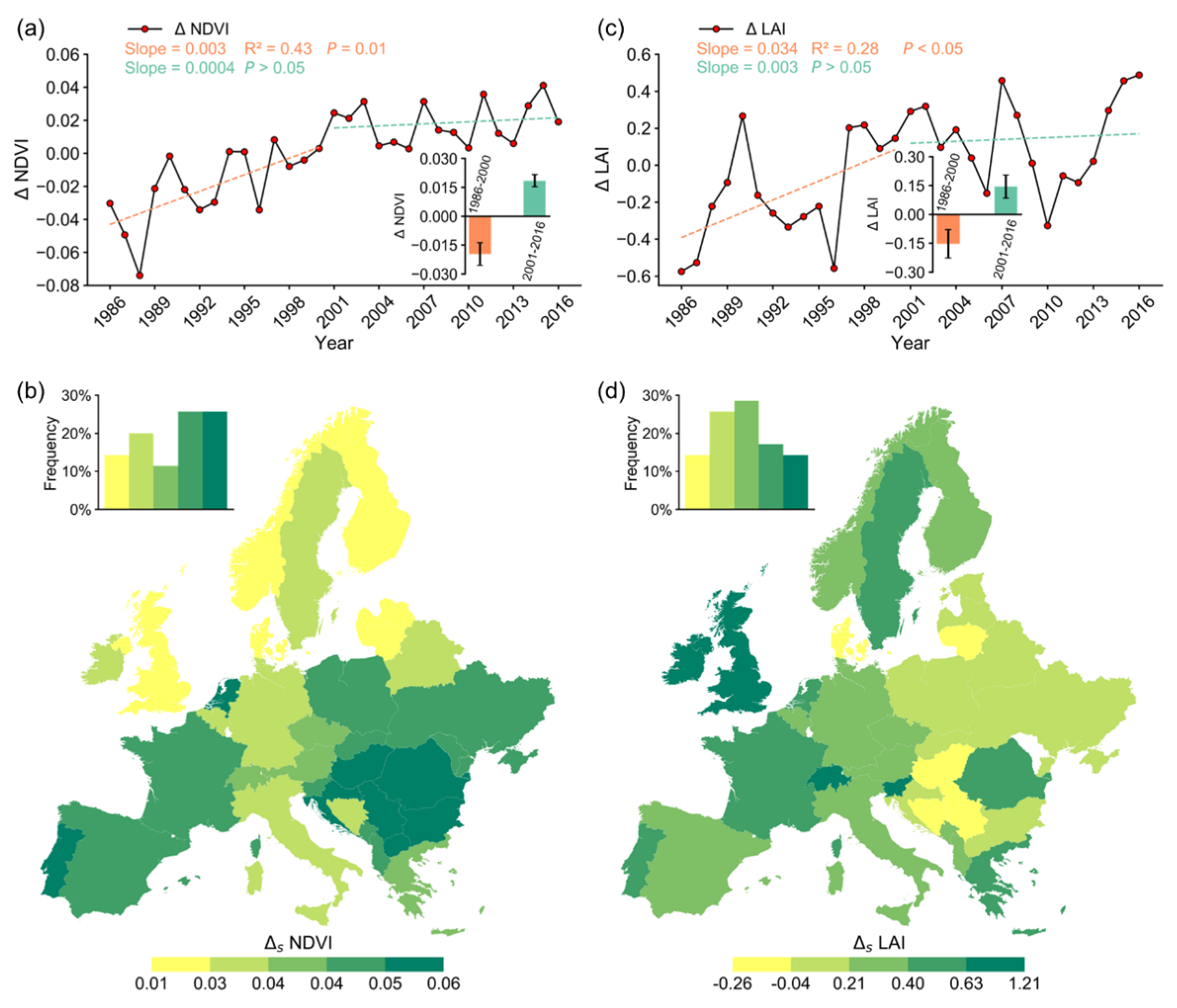
3.2. Spatiotemporal Patterns of Forest Biophysical Differences in Disturbance and Non-Disturbance

Both Δ NDVI and Δ LAI exhibited an overall increasing trend from 1986 to 2016, displaying similar temporal patterns within the 1986–2000 and 2001–2016 sub-periods (Figure 2). Δ NDVI and Δ LAI showed a significant increase (p < 0.05) in the former period, with slopes of 0.003 and 0.034, respectively. While, their trends stabilized during the 2001–2016 period, showing no statistically significant change (p > 0.05) (Figure 2a,c). Although Δ GPP also increased overall (from −1.93 ± 9.5 g C m⁻2 in 1986 to 1.72 ± 6.41 g C m⁻2 in 2016), no significant changes (p > 0.05) were detected within either sub-period (Figure S4).
In contrast, Δ Albedo and Δ ET demonstrated opposing dynamics between 1986 and 2016 (Figure 3). Δ Albedo showed a significant overall decrease, declining from 0.02 ± 0.01 in 1986 to −0.01 ± 0.01 in 2016 (Figure 3a). This decrease became more pronounced during 2001–2016 (slope = −0.001) compared to 1986–2000 (slope = −0.0002). Conversely, Δ ET exhibited a significant overall increase, rising from −27.66 ± 27.42 mm in 1986 to 35.65 ± 42.01 mm in 2016 (Figure 3c). This increase was substantial and statistically significant (p < 0.05) between 1986 and 2000 (slope = 1.937), after which no significant change (p > 0.05) was observed (post-2001).
The Δ s   NDVI , Δ s   LAI, Δ s Albedo, and Δ s   ET of the 35 European countries were not spatially homogeneous (Figure 2b,d and Figure 3b,d). The countries with larger Δ s   NDVI values are primarily located in the central and southern regions (Figure S3c). The countries with larger Δ s   LAI values are situated in the western region (Figure S3d). The countries with larger Δ s   Albedo values are situated in the central and southern regions (Figure S3e). The regions with larger Δ s   ET values are situated in the southeastern region (Figure S3f). The mean value of the Δ Albedo for all the countries was negative (−0.01), and the others were positive: Δ s   NDVI (0.04), Δ s   LAI (0.30), and Δ s   ET (33.74 mm) (Figure S5; Table S1).

3.3. The Temporal Variation in Climatic Factors

There were no statistically significant differences (p > 0.05) in the mean values of the key climatic factors between the 1986–2000 and 2001–2016 periods (Figures S6 and S7). Δ SWdown exhibited an increasing trend until 2000, followed by a decreasing trend after 2001. The other climatic factors experienced an increased trend in the two periods. The difference between climatic factors during the periods 1986~2000 and 1986~2000 are not significant (Table S2). The mean values of the Δ s   PDSI and Δ s SWdown for all the countries were negative, and the others were positive (Figure S8; Table S2).

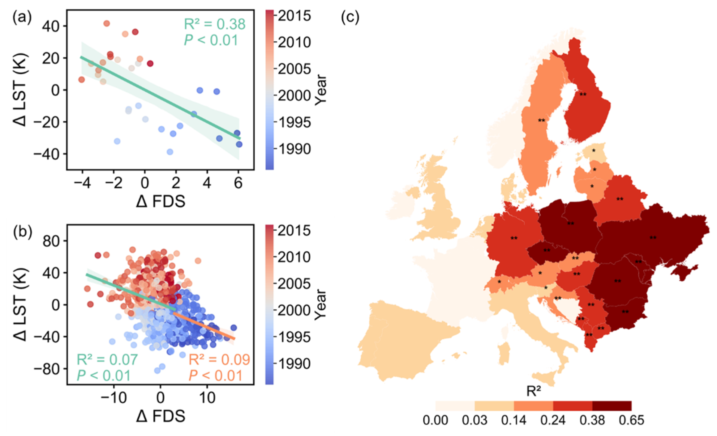
3.4. Correlation Between FDS on LST

A linear regression model was used to quantify the influence of FDS on the LST variations (Figure 4). The correlation between Δ FDS and Δ LST showed a significant (R2 = 0.38, p < 0.01) negative relationship (Figure 4a). Additionally, at a given stage, Δ FDS–Δ LST showed a significant negative correlation (p < 0.01); after 2001, Δ LST was generally higher. Moreover, the explanatory power of Δ FDS on Δ LST was stronger during the Δ FDS > 3 stage (R2 = 0.09) compared to that during the Δ FDS ≤ 3 stage (R2 = 0.07) (Figure 4b). Spatially, the correlation between Δ FDS and Δ LST was significant (p < 0.05) across extensive regions, with the strongest relationship predominantly observed in Central and Eastern Europe (Figure 4c).

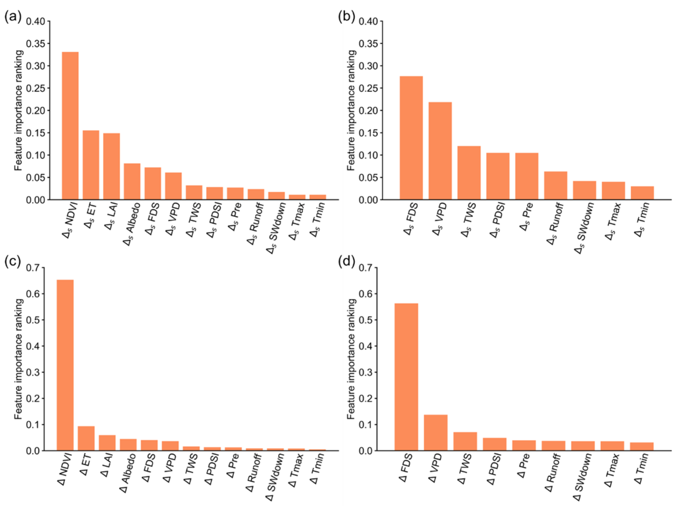
3.5. The Importance of Various Variables in Relation to LST and NDVI

RF analysis identified the primary drivers of LST and NDVI variations at the time series and national scales, respectively (Figure 5). The results highlighted the NDVI as the most important factor explaining Δ LST variability, while FDS was the principal factor explaining Δ NDVI variability. Specifically, the relative importance of the time series annual mean NDVI in explaining overall Δ LST (importance = 0.65) (Figure 5c) was markedly higher than its importance in explaining the national-scale change in Δ s   LST (importance = 0.33) (Figure 5a). Similarly, FDS showed higher importance in explaining the time series Δ NDVI (importance = 0.56) (Figure 5d) compared to the national-scale change in Δ s   NDVI (importance = 0.28) (Figure 5b). Considering these findings, alongside the observed decrease in FDS (Figure 1a) and the lack of significant differences (p > 0.05) in climatic factors (Figure S6) and TWS (Figure S7) between the 1986–2000 and 2001–2016 periods, the result suggests that FDS exerts a significant influence on LST, primarily mediated through its impact on the NDVI, rather than dominant influences from the background climate or soil moisture on the NDVI trends.

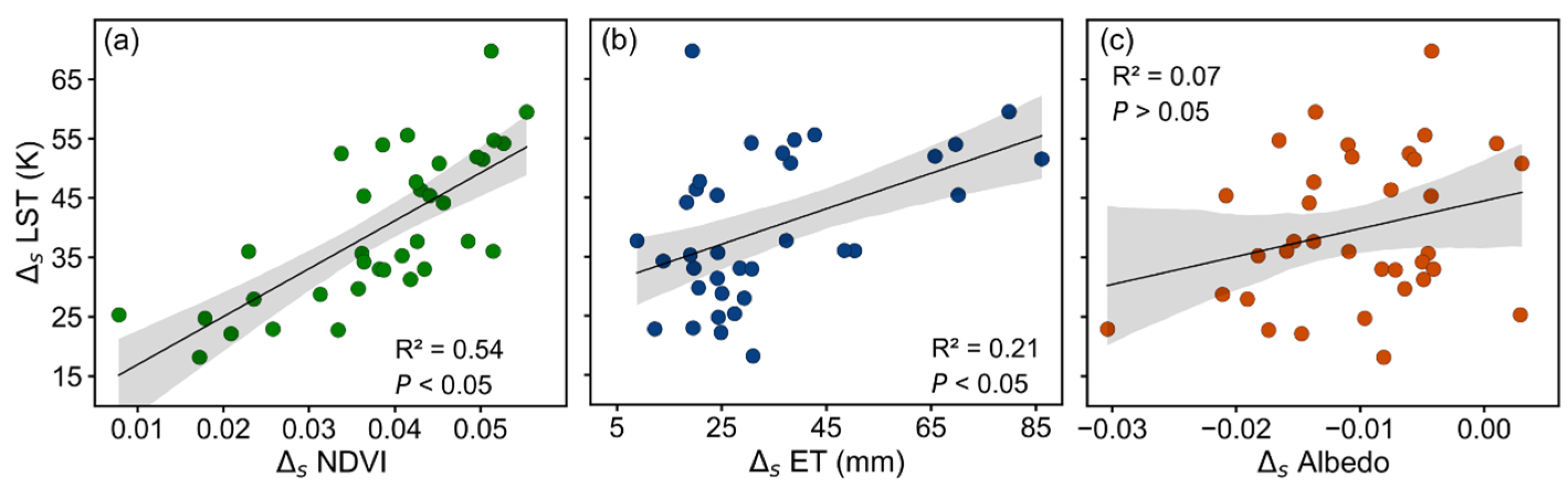
3.6. Correlations Between Δ LST and Δ NDVI, Δ ET, and Δ Albedo

Linear regression analysis elucidated the relationships between the inter-period change in LST and the corresponding changes in the associated variables (Figure 6). Significant positive correlations were identified between Δ s   LST and both the Δ s   NDVI (R2 = 0.54, p < 0.05) and Δ s   ET (R2 = 0.21, p < 0.05), with the strongest association observed for the Δ s   NDVI (Figure 6a,b). In contrast, no statistically significant linear relationship (p > 0.05) was found between Δ s   LST and Δ s   Albedo (R2 = 0.07) (Figure 6c). But, there was a significant linear relationship (R2 = 0.38, p < 0.01) between Δ LST and Δ Albedo based on the time scale (Figure S9).

4. Discussion

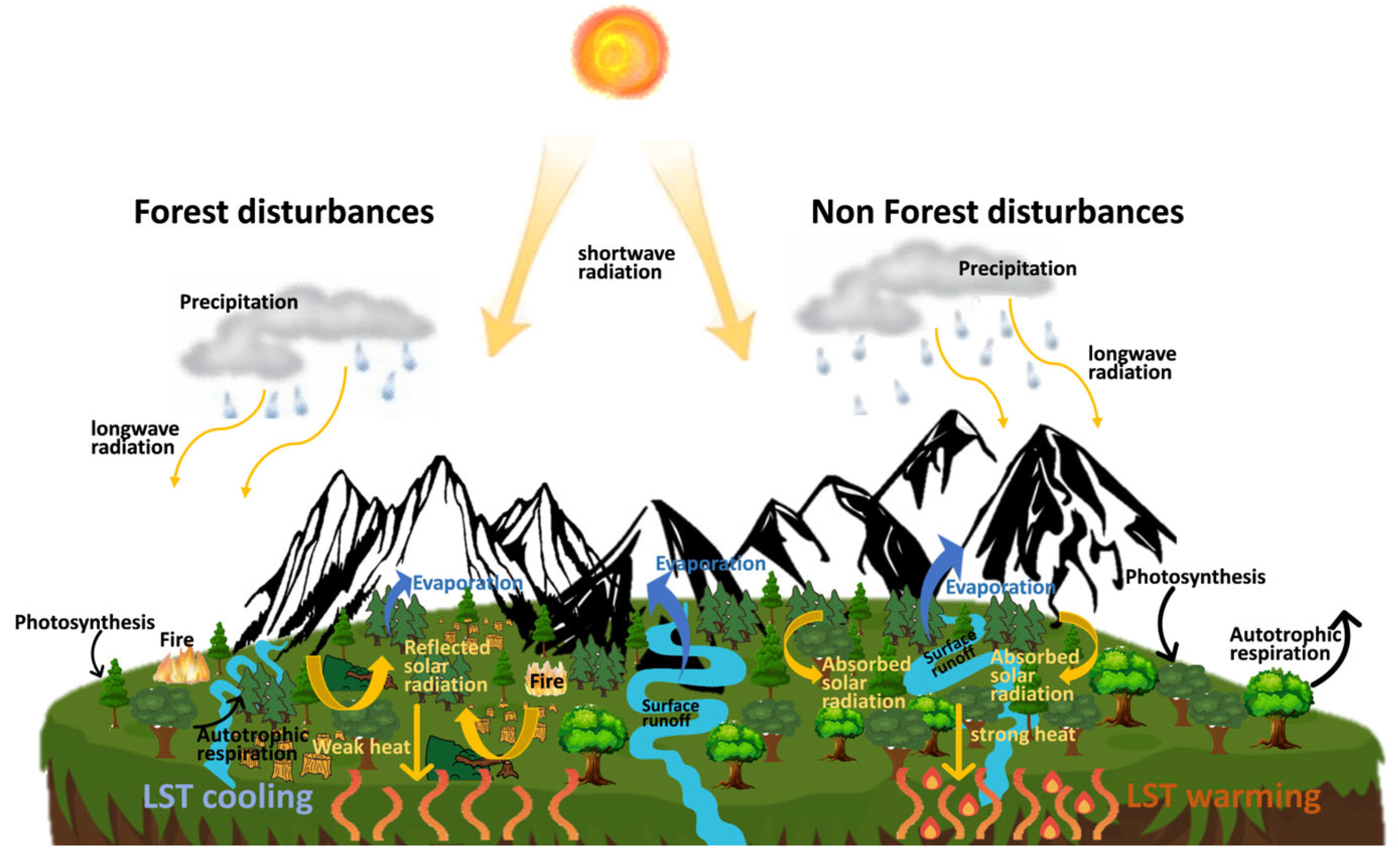
4.1. Potential Mechanisms of FDS Dominance of LST

Our findings suggest that FDS dynamics strongly influenced LST over the European continent, contributing to a significant warming trend observed from 1986 to 2016. This trend (Figure 7) is attributable to biogeophysical feedback mechanisms; sustained increases in forest LAI led to reduced surface albedo, consequently amplifying surface warming via the enhanced absorption of shortwave radiation. This interpretation aligns with multi-scale satellite observations documenting a widespread global vegetation greening trend in recent decades [51,52,53]. Although the drivers of global greening are regionally heterogeneous [54], involving factors such as CO2 fertilization [51,53,54], nitrogen deposition [53], climate change [52,53,54,55,56], and land cover changes [53,57], our attribution analysis reveals a distinct characteristic for Europe. The RF models demonstrate that forest expansion in this region during 1986–2016 was primarily driven by FDS rather than the conventionally recognized climatic factors. This finding contrasts sharply with Zhu et al. [53]’s conclusion that high-latitude greening is mainly climate-driven, suggesting potential unique regulatory mechanisms in European forest dynamics. From a biophysical perspective, forest dynamics significantly modulate the surface energy balance by altering key parameters like surface albedo and evapotranspiration [1,6,16,17], inducing net warming or cooling effects [58]. This study quantifies these competing processes, showing that the positive radiative forcing from albedo reduction intensifies with latitude, while negative forcing from increased ET diminishes poleward. This spatial heterogeneity results in the warming effect dominated by albedo changes prevailing over the cooling effect from ET across the European continent. These findings corroborate those of Li et al. [15] and underscore the crucial role of FDS-related forest dynamics in modulating European continental climate change.

4.2. Implications

This research underscores the pivotal role of FDS dynamics in modulating LST evolution across Europe. The scientific and practical significance lies in three key contributions: (1) Methodological advancement—Moving beyond the traditional climate model-based analyses [59], this work pioneers an integrative approach using multi-source remote sensing data. This provides the first quantitative, continent-wide characterization of forest–LST relationships for Europe, effectively addressing the inadequate representation of localized biophysical effects in simulations. (2) Enhanced mechanistic understanding—Through multi-scale spatiotemporal analysis, this study corroborates the positive association between increased forest cover (linked to FDS recovery dynamics) and LST [16,17,60]. Crucially, it elucidates the underpinning biophysical mechanism, forest expansion and densification reduce surface albedo, leading to the enhanced absorption of shortwave radiation and consequent local warming [5,61], thereby advancing the fundamental understanding of land–atmosphere interactions. (3) Guidance for sustainable management—The quantitative framework linking forest dynamics (influenced by FDS changes) to LST responses provides an empirical foundation for precision forest management. This understanding enables policymakers to better optimize forestry activities (e.g., afforestation and harvesting) by balancing the carbon sequestration objectives with biophysical climate impacts, offering vital decision support for achieving Europe’s climate goals. Collectively, these findings deepen the understanding of ecosystem–climate feedback mechanisms and provide both a robust theoretical basis and practical guidance for sustainable forest management and regional climate adaptation strategies.

4.3. Uncertainties in This Study

The reliability of the conclusions in this study may be influenced by three key uncertainty factors: (1) Limitations of annual average and national-scale aggregation calculation methods—In order to understand the FDS-LST mechanism at the macro scale and to facilitate the provision of a scientific basis for wannabe policymakers, we chose both the time series (annual mean) and national scales. Time series (annual mean) may blur the mean values over the period of active vegetation. The direct physiological activity of vegetation predominantly occurs during the growing season; non-growing-season climatic conditions (e.g., winter temperatures) may exert lagged effects on subsequent growing seasons (e.g., influencing spring phenology) [62]. Analyzing FDS at the national scale may mask local heterogeneities in vegetation–climate interactions, potentially introducing biases. Future research should leverage geographically weighted regression (GWR) models to account for spatial non-stationarity, integrated with multi-scale spatial analysis techniques [63,64,65]. Sensitivity analyses across varying spatial resolutions are also crucial to validate the robustness of the findings. (2) Limitations in environmental variable representation—The current framework does not fully incorporate dynamic environmental drivers, such as the frequency and intensity of extreme climate events [66], policy interventions, and human activity patterns (e.g., night-time light data, GDP gradients, and population density). Developing dynamic coupled models that integrate socioeconomic factors and establishing a more comprehensive multi-dimensional environmental variable index system would enhance the explanatory power in future studies. (3) Neglecting the biochemical feedback of forest disturbance with climate—This research concentrated on the biophysical regulation of LST by forest cover changes (e.g., albedo–evapotranspiration balance), excluding the biogeochemical feedback associated with rising atmospheric CO2 (e.g., CO2 fertilization effects) [5]. This decoupling may lead to the underestimation of the net surface temperature response. Implementing multi-scenario simulations with earth system models is recommended for future work to disentangle and quantify the relative contributions of different climate feedback pathways. (4) In Section 2.7, we rely on human designation for the division of the time series and do not fully show the data trends; this was conducted to balance the sample size to facilitate the development of a forest management policy in Europe. Liu et al. [67] used segmented linear regression for the time series intervals, which provides some reference for our subsequent study.

5. Conclusions

Leveraging high-resolution (30 m) forest disturbance datasets from 1986 to 2016, integrated with multi-source remote sensing observations (LST, NDVI, LAI, albedo, and ET), this study provides the first systematic, continental-scale elucidation of the multidimensional LST response to FDS across Europe. By statistically disentangling the influence of climate variability, our analysis demonstrates that forest disturbance dynamics were the primary driver of the observed LST increases in continental Europe during this period, with their contribution significantly exceeding the independent impacts of climate change. Temporal analysis revealed a significant overall decrease in European FDS, although this decline markedly decelerated after 2001, offering novel quantitative insights into the evolving resilience of European forest ecosystems. Mechanistically, this research identified dual pathways through which individual forest disturbance events impact LST: (1) immediate alterations to the land surface energy balance (e.g., increased albedo and reduced evapotranspiration) and (2) modifications to the vegetation structure and physiology (e.g., a reduced NDVI and LAI). These findings provide critical parameters for refining land–atmosphere interaction models and offer a robust scientific foundation for the European Union’s implementation of nature-based solutions (NBSs) to achieve the climate objectives of The Paris Agreement and develop climate-resilient forest management systems.

Supplementary Materials

The following supporting information can be downloaded at: https://www.mdpi.com/article/10.3390/f16050852/s1, Figure S1: Example of 3 × 3 matrix with the disturbed pixels between 1986~2016. Orange indicates a pixel classified as disturbed within this period, while green indicates an undisturbed pixel. Pixels are numbered P1 through P9 for reference, with P5 typically representing the central target pixel; Table S1: The mean values of Δ for FDS, LST, Albedo, ET and vegetation factors between (1986~2000) and (2001~2016) and the mean values of Δ s for all European countries; Figure S2: Time series of Tmax and Tmin in Europe from 1986 to 2016. (a) Δ Tmax time series; (b) Comparison of mean Δ Tmax values between the periods 1986–2000 and 2001–2016; (c) Δ Tmin time series; (d) Comparison of mean Δ Tmin values between the periods 1986–2000 and 2001–2016. Orange and green dashed lines represent the linear regression lines fitted to the data for the 1986–2000 and 2001–2016 periods, respectively; Table S2: The mean values of Δ for climatic factors between (1986~2000) and (2001~2016) and the mean values of Δ s for all European countries; Figure S3: Top 10 European countries ranked by the magnitude of the inter-period difference ( Δ s variable, calculated as mean 2001–2016 minus mean 1986–2000) for selected variables. (a) Ranking by Δ s FDS; (b) Ranking by Δ s LST; (c) Ranking by Δ s NDVI; (d) Ranking by Δ s LAI; (e) Ranking by Δ s Albedo; (f) Ranking by Δ s ET; Figure S4: Time series analysis of Δ GPP in Europe from 1986 to 2016. (a) Time series of Δ GPP; (b) Comparison of mean Δ GPP values between the periods 1986–2000 and 2001–2016. Orange and green dashed lines represent the linear regression lines fitted to the data for the 1986–2000 and 2001–2016 periods, respectively; Figure S5: The mean values of Δ s   LST , Δ s   FDS , Δ s   NDVI , Δ s   LAI , Δ s   Albedo , Δ s   ET for all European countries; Figure S6: Time series analysis of climate factor differences (Δ Variable) in Europe from 1986 to 2016. (a) Δ Pre time series; (b) Comparison of mean Δ Pre between 1986–2000 and 2001–2016; (c) Δ SWdown time series; (d) Comparison of mean Δ SWdown between 1986–2000 and 2001–2016; (e) Δ VPD time series; (f) The mean values of Δ VPD between (1986~2000) and (2001~2016); (g) Δ PDSI time series; (h) Comparison of mean Δ PDSI between 1986–2000 and 2001–2016. Orange and green dashed lines represent the linear regression lines fitted to the data for the 1986–2000 and 2001–2016 periods, respectively; Figure S7: Time series of Δ TWS and Δ Runoff in Europe between 1986 to 2016. (a) Δ TWS time series; (b) Comparison of mean Δ TWS values between 1986–2000 and 2001–2016; (c) Δ Runoff time series; (d) Comparison of mean Δ Runoff between 1986–2000 and 2001–2016. Orange and green dashed lines represent the linear regression lines fitted to the data for the 1986–2000 and 2001–2016 periods, respectively; Figure S8: The mean values of Δ s   Pre , Δ s   SWdown , Δ s   VPD , Δ s   PDSI , Δ s   TWS , Δ s   Runoff for all European countries; Figure S9: The relationship between Δ LST and Δ Albedo.

Author Contributions

Conceptualization, W.Z. and X.C.; methodology, W.Z. and Y.Z.; software, W.Z.; validation, W.Z., Y.Z. and X.C.; formal analysis, W.Z.; investigation, W.Z.; resources, W.Z.; data curation, W.Z.; writing—original draft preparation, W.Z.; writing—review and editing, Y.Z. and X.C.; visualization, W.Z.; supervision, Y.Z. and X.C.; project administration, Y.Z. and X.C.; funding acquisition, X.C. All authors have read and agreed to the published version of the manuscript.

Funding

This research was funded by National Key R&D Program of China (No. 2024YFF1306600) and the Science and Technology Program of Guangdong (No. 2024B1212070012).

Data Availability Statement

The original contributions presented in this study are included in the article. Further inquiries can be directed to the corresponding author.

Acknowledgments

We sincerely appreciate the editors and the anonymous reviewers for their valuable comments.

Conflicts of Interest

The authors declare no conflicts of interest.

References

  1. Bonan, G.B. Forests and Climate Change: Forcings, Feedbacks, and the Climate Benefits of Forests. Science 2008, 320, 1444–1449. [Google Scholar] [CrossRef] [PubMed]
  2. Senf, C.; Seidl, R. Mapping the Forest Disturbance Regimes of Europe. Nat Sustain. 2021, 4, 63–70. [Google Scholar] [CrossRef]
  3. Anderson, R.G.; Canadell, J.G.; Randerson, J.T.; Jackson, R.B.; Hungate, B.A.; Baldocchi, D.D.; Ban-Weiss, G.A.; Bonan, G.B.; Caldeira, K.; Cao, L.; et al. Biophysical Considerations in Forestry for Climate Protection. Front. Ecol. Environ. 2011, 9, 174–182. [Google Scholar] [CrossRef]
  4. Marland, G.; Pielke, R.A.; Apps, M.; Avissar, R.; Betts, R.A.; Davis, K.J.; Frumhoff, P.C.; Jackson, S.T.; Joyce, L.A.; Kauppi, P.; et al. The Climatic Impacts of Land Surface Change and Carbon Management, and the Implications for Climate-Change Mitigation Policy. Clim. Policy 2003, 3, 149–157. [Google Scholar] [CrossRef]
  5. Bala, G.; Caldeira, K.; Wickett, M.; Phillips, T.J.; Lobell, D.B.; Delire, C.; Mirin, A. Combined Climate and Carbon-Cycle Effects of Large-Scale Deforestation. Proc. Natl. Acad. Sci. USA 2007, 104, 6550–6555. [Google Scholar] [CrossRef]
  6. Windisch, M.G.; Davin, E.L.; Seneviratne, S. Prioritizing Forestation Based on Biogeochemical and Local Biogeophysical Impacts. Nat. Clim. Chang. 2021, 11, 867–871. [Google Scholar] [CrossRef]
  7. Friedlingstein, P.; O’Sullivan, M.; Jones, M.W.; Andrew, R.M.; Gregor, L.; Hauck, J.; Le Quere, C.; Luijkx, I.T.; Olsen, A.; Peters, G.P.; et al. Global Carbon Budget 2022. Earth Syst. Sci. Data 2022, 14, 4811–4900. [Google Scholar] [CrossRef]
  8. Pugh, T.A.M.; Arneth, A.; Kautz, M.; Poulter, B.; Smith, B. Important Role of Forest Disturbances in the Global Biomass Turnover and Carbon Sinks. Nat. Geosci. 2019, 12, 730–735. [Google Scholar] [CrossRef]
  9. Silva Junior, C.H.L.; Carvalho, N.S.; Pessoa, A.C.M.; Reis, J.B.C.; Pontes-Lopes, A.; Doblas, J.; Heinrich, V.; Campanharo, W.; Alencar, A.; Silva, C.; et al. Amazonian Forest Degradation Must Be Incorporated into the COP26 Agenda. Nat. Geosci. 2021, 14, 634–635. [Google Scholar] [CrossRef]
  10. Jackson, R.B.; Randerson, J.T.; Canadell, J.G.; Anderson, R.G.; Avissar, R.; Baldocchi, D.D.; Bonan, G.B.; Caldeira, K.; Diffenbaugh, N.S.; Field, C.B.; et al. Protecting Climate with Forests. Environ. Res. Lett. 2008, 3, 044006. [Google Scholar] [CrossRef]
  11. Rotenberg, E.; Yakir, D. Contribution of Semi-Arid Forests to the Climate System. Science 2010, 327, 451–454. [Google Scholar] [CrossRef] [PubMed]
  12. Betts, R.A. Offset of the Potential Carbon Sink from Boreal Forestation by Decreases in Surface Albedo. Nature 2000, 408, 187–190. [Google Scholar] [CrossRef] [PubMed]
  13. Bright, R.M.; Zhao, K.; Jackson, R.B.; Cherubini, F. Quantifying surface albedo and other direct biogeophysical climate forcings of forestry activities. Glob. Change Biol. 2015, 21, 3246–3266. [Google Scholar] [CrossRef]
  14. Loranty, M.M.; Goetz, S.J.; Beck, P.S. Tundra vegetation effects on pan-Arctic albedo. Environ. Res. Lett. 2011, 6, 024014. [Google Scholar] [CrossRef]
  15. Li, Y.; Zhao, M.; Motesharrei, S.; Mu, Q.; Kalnay, E.; Li, S. Local Cooling and Warming Effects of Forests Based on Satellite Observations. Nat. Commun. 2015, 6, 6603. [Google Scholar] [CrossRef]
  16. Peng, S.-S.; Piao, S.; Zeng, Z.; Ciais, P.; Zhou, L.; Li, L.Z.X.; Myneni, R.B.; Yin, Y.; Zeng, H. Afforestation in China Cools Local Land Surface Temperature. Proc. Natl. Acad. Sci. USA 2014, 111, 2915–2919. [Google Scholar] [CrossRef]
  17. Schmidt, M.; Jochheim, H.; Kersebaum, K.-C.; Lischeid, G.; Nendel, C. Gradients of Microclimate, Carbon and Nitrogen in Transition Zones of Fragmented Landscapes—A Review. Agric. For. Meteorol. 2017, 232, 659–671. [Google Scholar] [CrossRef]
  18. Zhu, L.; Li, W.; Ciais, P.; He, J.; Cescatti, A.; Santoro, M.; Tanaka, K.; Cartus, O.; Zhao, Z.; Xu, Y.; et al. Comparable Biophysical and Biogeochemical Feedbacks on Warming from Tropical Moist Forest Degradation. Nat. Geosci. 2023, 16, 244–249. [Google Scholar] [CrossRef]
  19. Seidl, R.; Thom, D.; Kautz, M.; Martin-Benito, D.; Peltoniemi, M.; Vacchiano, G.; Wild, J.; Ascoli, D.; Petr, M.; Honkaniemi, J.; et al. Forest Disturbances under Climate Change. Nat. Clim. Chang. 2017, 7, 395–402. [Google Scholar] [CrossRef]
  20. Schelhaas, M.; Nabuurs, G.; Schuck, A. Natural Disturbances in the European Forests in the 19th and 20th Centuries. Glob. Change Biol. 2003, 9, 1620–1633. [Google Scholar] [CrossRef]
  21. Nabuurs, G.-J.; Lindner, M.; Verkerk, P.J.; Gunia, K.; Deda, P.; Michalak, R.; Grassi, G. First Signs of Carbon Sink Saturation in European Forest Biomass. Nat. Clim. Chang. 2013, 3, 792–796. [Google Scholar] [CrossRef]
  22. Gutschick, V.P.; BassiriRad, H. Extreme Events as Shaping Physiology, Ecology, and Evolution of Plants: Toward a Unified Definition and Evaluation of Their Consequences. New Phytol. 2003, 160, 21–42. [Google Scholar] [CrossRef] [PubMed]
  23. Patacca, M.; Lindner, M.; Lucas-Borja, M.E.; Cordonnier, T.; Fidej, G.; Gardiner, B.; Hauf, Y.; Jasinevičius, G.; Labonne, S.; Linkevičius, E.; et al. Significant Increase in Natural Disturbance Impacts on European Forests since 1950. Glob. Change Biol. 2023, 29, 1359–1376. [Google Scholar] [CrossRef] [PubMed]
  24. Suvanto, S.; Lehtonen, A.; Nevalainen, S.; Lehtonen, I.; Viiri, H.; Strandström, M.; Peltoniemi, M. Mapping the Probability of Forest Snow Disturbances in Finland. PLoS ONE 2021, 16, e0254876. [Google Scholar]
  25. Lehtonen, I.; Kämäräinen, M.; Gregow, H.; Venäläinen, A.; Peltola, H. Heavy Snow Loads in Finnish Forests Respond Regionally Asymmetrically to Projected Climate Change. Nat. Hazards Earth Syst. Sci. 2016, 16, 2259–2271. [Google Scholar] [CrossRef]
  26. Nagel, T.A.; Mikac, S.; Dolinar, M.; Klopcic, M.; Keren, S.; Svoboda, M.; Diaci, J.; Boncina, A.; Paulic, V. The Natural Disturbance Regime in Forests of the Dinaric Mountains: A Synthesis of Evidence. For. Ecol. Manag. 2017, 388, 29–42. [Google Scholar] [CrossRef]
  27. Amiro, B.D.; Orchansky, A.L.; Barr, A.G.; Black, T.A.; Chambers, S.D.; Chapin Iii, F.S.; Goulden, M.L.; Litvak, M.; Liu, H.P.; McCaughey, J.H.; et al. The Effect of Post-Fire Stand Age on the Boreal Forest Energy Balance. Agric. For. Meteorol. 2006, 140, 41–50. [Google Scholar] [CrossRef]
  28. Govindasamy, B.; Duffy, P.B.; Caldeira, K. Land Use Changes and Northern Hemisphere Cooling. Geophys. Res. Lett. 2001, 28, 291–294. [Google Scholar] [CrossRef]
  29. Lee, X.; Goulden, M.L.; Hollinger, D.Y.; Barr, A.; Black, T.A.; Bohrer, G.; Bracho, R.; Drake, B.; Goldstein, A.; Gu, L.; et al. Observed Increase in Local Cooling Effect of Deforestation at Higher Latitudes. Nature 2011, 479, 384–387. [Google Scholar] [CrossRef]
  30. Dalmonech, D.; Marano, G.; Amthor, J.S.; Cescatti, A.; Lindner, M.; Trotta, C.; Collalti, A. Feasibility of Enhancing Carbon Sequestration and Stock Capacity in Temperate and Boreal European Forests via Changes to Management Regimes. Agric. For. Meteorol. 2022, 327, 109203. [Google Scholar] [CrossRef]
  31. Grünig, M.; Seidl, R.; Senf, C. Increasing Aridity Causes Larger and More Severe Forest Fires across Europe. Glob. Change Biol. 2023, 29, 1648–1659. [Google Scholar] [CrossRef] [PubMed]
  32. Kebrle, D.; Zasadil, P.; Barták, V.; Hofmeister, J. Bird Response to Forest Disturbance Size in Mountain Spruce Forests in Central Europe. For. Ecol. Manag. 2022, 524, 120527. [Google Scholar] [CrossRef]
  33. Liu, Q.; Wang, L.; Qu, Y.; Liu, N.; Liu, S.; Tang, H.; Liang, S. Preliminary Evaluation of the Long-Term GLASS Albedo Product. Int. J. Digit. Earth 2013, 6, 69–95. [Google Scholar] [CrossRef]
  34. Liu, X.; Tang, B.-H.; Yan, G.; Li, Z.-L.; Liang, S. Retrieval of Global Orbit Drift Corrected Land Surface Temperature from Long-Term AVHRR Data. Remote Sens. 2019, 11, 2843. [Google Scholar] [CrossRef]
  35. Xiao, Z.; Liang, S.; Wang, J.; Xiang, Y.; Zhao, X.; Song, J. Long-Time-Series Global Land Surface Satellite Leaf Area Index Product Derived From MODIS and AVHRR Surface Reflectance. IEEE Trans. Geosci. Remote Sens. 2016, 54, 5301–5318. [Google Scholar] [CrossRef]
  36. Xiao, Z.; Liang, S.; Wang, J.; Chen, P.; Yin, X.; Zhang, L.; Song, J. Use of General Regression Neural Networks for Generating the GLASS Leaf Area Index Product From Time-Series MODIS Surface Reflectance. IEEE Trans. Geosci. Remote Sens. 2014, 52, 209–223. [Google Scholar] [CrossRef]
  37. Yuan, W.; Liu, S.; Yu, G.; Bonnefond, J.-M.; Chen, J.; Davis, K.; Desai, A.R.; Goldstein, A.H.; Gianelle, D.; Rossi, F.; et al. Global Estimates of Evapotranspiration and Gross Primary Production Based on MODIS and Global Meteorology Data. Remote Sens. Environ. 2010, 114, 1416–1431. [Google Scholar] [CrossRef]
  38. Li, Y.; Zhao, M.; Mildrexler, D.J.; Motesharrei, S.; Mu, Q.; Kalnay, E.; Zhao, F.; Li, S.; Wang, K. Potential and Actual Impacts of Deforestation and Afforestation on Land Surface Temperature. J. Geophys. Res. 2016, 121, 14372–14386. [Google Scholar] [CrossRef]
  39. Abatzoglou, J.T.; Dobrowski, S.Z.; Parks, S.A.; Hegewisch, K.C. Data Descriptor: TerraClimate, a High-Resolution Global Dataset of Monthly Climate and Climatic Water Balance from 1958–2015. Sci. Data 2018, 5, 170191. [Google Scholar] [CrossRef]
  40. Abatzoglou, J.T.; Williams, A.P.; Boschetti, L.; Zubkova, M.; Kolden, C.A. Global Patterns of Interannual Climate-Fire Relationships. Glob. Change Biol. 2018, 24, 5164–5175. [Google Scholar] [CrossRef]
  41. Yuan, W.; Zheng, Y.; Piao, S.; Ciais, P.; Lombardozzi, D.; Wang, Y.; Ryu, Y.; Chen, G.; Dong, W.; Hu, Z.; et al. Increased Atmospheric Vapor Pressure Deficit Reduces Global Vegetation Growth. Sci. Adv. 2019, 5, eaax1396. [Google Scholar] [CrossRef] [PubMed]
  42. Humphrey, V.; Gudmundsson, L. GRACE-REC: A Reconstruction of Climate-Driven Water Storage Changes over the Last Century. Earth Syst. Sci. Data 2019, 11, 1153–1170. [Google Scholar] [CrossRef]
  43. Zhao, H.; Zhang, Z.; Ying, H.; Chen, J.; Zhen, S.; Wang, X.; Shan, Y. The Spatial Patterns of Climate-Fire Relationships on the Mongolian Plateau. Agric. For. Meteorol. 2021, 308, 108549. [Google Scholar] [CrossRef]
  44. Yu, L.; Fan, L.; Ciais, P.; Sitch, S.; Fensholt, R.; Xiao, X.; Yuan, W.; Chen, J.; Zhang, Y.; Wu, X.; et al. Carbon Dynamics of Western North American Boreal Forests in Response to Stand-Replacing Disturbances. Int. J. Appl. Earth Obs. Geoinf. 2023, 122, 103410. [Google Scholar] [CrossRef]
  45. Danneyrolles, V.; Boucher, Y.; Fournier, R.; Valeria, O. Positive Effects of Projected Climate Change on Post-Disturbance Forest Regrowth Rates in Northeastern North American Boreal Forests. Environ. Res. Lett. 2023, 18, 024041. [Google Scholar] [CrossRef]
  46. Dobor, L.; Hlásny, T.; Rammer, W.; Barka, I.; Trombik, J.; Pavlenda, P.; Šebeň, V.; Štěpánek, P.; Seidl, R. Post-Disturbance Recovery of Forest Carbon in a Temperate Forest Landscape under Climate Change. Agric. For. Meteorol. 2018, 263, 308–322. [Google Scholar] [CrossRef]
  47. Cuevas-González, M.; Gerard, F.; Balzter, H.; Riaño, D. Analysing Forest Recovery after Wildfire Disturbance in Boreal Siberia Using Remotely Sensed Vegetation Indices. Glob. Change Biol. 2009, 15, 561–577. [Google Scholar] [CrossRef]
  48. Ma, T.; Liang, Y.; Li, Z.; Liu, Z.; Liu, B.; Wu, M.M.; Lau, M.K.; Fang, Y. Age-Related Patterns and Climatic Driving Factors of Drought-Induced Forest Mortality in Northeast China. Agric. For. Meteorol. 2023, 332, 109360. [Google Scholar] [CrossRef]
  49. Wu, C.; Hou, X.; Peng, D.; Gonsamo, A.; Xu, S. Land Surface Phenology of China’s Temperate Ecosystems over 1999–2013: Spatial–Temporal Patterns, Interaction Effects, Covariation with Climate and Implications for Productivity. Agric. For. Meteorol. 2016, 216, 177–187. [Google Scholar] [CrossRef]
  50. Breiman, L. Random Forests. Mach. Learn. 2001, 45, 5–32. [Google Scholar] [CrossRef]
  51. Buitenwerf, R.; Sandel, B.; Normand, S.; Mimet, A.; Svenning, J. Land Surface Greening Suggests Vigorous Woody Regrowth throughout European Semi-natural Vegetation. Glob. Change Biol. 2018, 24, 5789–5801. [Google Scholar] [CrossRef] [PubMed]
  52. Zhou, L.; Tucker, C.J.; Kaufmann, R.K.; Slayback, D.; Shabanov, N.V.; Myneni, R.B. Variations in Northern Vegetation Activity Inferred from Satellite Data of Vegetation Index during 1981 to 1999. J. Geophys. Res. 2001, 106, 20069–20083. [Google Scholar] [CrossRef]
  53. Zhu, Z.; Piao, S.; Myneni, R.B.; Huang, M.; Zeng, Z.; Canadell, J.G.; Ciais, P.; Sitch, S.; Friedlingstein, P.; Arneth, A.; et al. Greening of the Earth and Its Drivers. Nat. Clim. Chang. 2016, 6, 791–795. [Google Scholar] [CrossRef]
  54. Chen, C.; Park, T.; Wang, X.; Piao, S.; Xu, B.; Chaturvedi, R.K.; Fuchs, R.; Brovkin, V.; Ciais, P.; Fensholt, R.; et al. China and India Lead in Greening of the World through Land-Use Management. Nat. Sustain. 2019, 2, 122–129. [Google Scholar] [CrossRef]
  55. Fensholt, R.; Langanke, T.; Rasmussen, K.; Reenberg, A.; Prince, S.D.; Tucker, C.; Scholes, R.J.; Le, Q.B.; Bondeau, A.; Eastman, R.; et al. Greenness in Semi-Arid Areas across the Globe 1981–2007—An Earth Observing Satellite Based Analysis of Trends and Drivers. Remote Sens. Environ. 2012, 121, 144–158. [Google Scholar] [CrossRef]
  56. Xu, L.; Myneni, R.B.; Chapin Iii, F.S.; Callaghan, T.V.; Pinzon, J.E.; Tucker, C.J.; Zhu, Z.; Bi, J.; Ciais, P.; Tømmervik, H.; et al. Temperature and Vegetation Seasonality Diminishment over Northern Lands. Nat. Clim. Chang. 2013, 3, 581–586. [Google Scholar] [CrossRef]
  57. Liu, Y.; Li, Y.; Li, S.; Motesharrei, S. Spatial and Temporal Patterns of Global NDVI Trends: Correlations with Climate and Human Factors. Remote Sens. 2015, 7, 13233–13250. [Google Scholar] [CrossRef]
  58. Gibbard, S.; Caldeira, K.; Bala, G.; Phillips, T.J.; Wickett, M. Climate Effects of Global Land Cover Change. Geophys. Res. Lett. 2005, 32, 2005GL024550. [Google Scholar] [CrossRef]
  59. Winckler, J.; Lejeune, Q.; Reick, C.H.; Pongratz, J. Nonlocal Effects Dominate the Global Mean Surface Temperature Response to the Biogeophysical Effects of Deforestation. Geophys. Res. Lett. 2019, 46, 745–755. [Google Scholar] [CrossRef]
  60. Montenegro, A.; Eby, M.; Mu, Q.; Mulligan, M.; Weaver, A.J.; Wiebe, E.C.; Zhao, M. The Net Carbon Drawdown of Small Scale Afforestation from Satellite Observations. Glob. Planet. Chang. 2009, 69, 195–204. [Google Scholar] [CrossRef]
  61. West, P.C.; Narisma, G.T.; Barford, C.C.; Kucharik, C.J.; Foley, J.A. An Alternative Approach for Quantifying Climate Regulation by Ecosystems. Front. Ecol. Environ. 2011, 9, 126–133. [Google Scholar] [CrossRef]
  62. Menzel, A.; Sparks, T.H.; Estrella, N.; Koch, E.; Aasa, A.; Ahas, R.; Zust, A.N.A. European phenological response to climate change matches the warming pattern. Glob. Change Biol. 2006, 12, 1969–1976. [Google Scholar] [CrossRef]
  63. Falk, D.A.; Miller, C.; McKenzie, D.; Black, A.E. Cross-Scale Analysis of Fire Regimes. Ecosystems 2007, 10, 809–823. [Google Scholar] [CrossRef]
  64. Parisien, M.-A.; Moritz, M.A. Environmental Controls on the Distribution of Wildfire at Multiple Spatial Scales. Ecol. Monogr. 2009, 79, 127–154. [Google Scholar] [CrossRef]
  65. Urbieta, I.R.; Zavala, G.; Bedia, J.; Gutiérrez, J.M.; Miguel-Ayanz, J.S.; Camia, A.; Keeley, J.E.; Moreno, J.M. Fire Activity as a Function of Fire–Weather Seasonal Severity and Antecedent Climate across Spatial Scales in Southern Europe and Pacific Western USA. Environ. Res. Lett. 2015, 10, 114013. [Google Scholar] [CrossRef]
  66. Li, C.; Filho, W.L.; Wang, J.; Yin, J.; Fedoruk, M.; Bao, G.; Bao, Y.; Yin, S.; Yu, S.; Hu, R. An Assessment of the Impacts of Climate Extremes on the Vegetation in Mongolian Plateau: Using a Scenarios-Based Analysis to Support Regional Adaptation and Mitigation Options. Ecol. Indic. 2018, 95, 805–814. [Google Scholar] [CrossRef]
  67. Liu, Q.; Peng, C.; Schneider, R.; Cyr, D.; McDowell, N.G.; Kneeshaw, D. Drought-induced increase in tree mortality and corresponding decrease in the carbon sink capacity of Canada’s boreal forests from 1970 to 2020. Glob. Change Biol. 2019, 29, 2274–2285. [Google Scholar] [CrossRef]
Figure 1. Spatiotemporal patterns of Δ FDS and Δ LST in Europe between 1986 and 2016. (a) Δ FDS time series. (b) Spatial patterns of Δ s   FDS . (c) Δ LST time series. (d) Spatial patterns of Δ s   LST. Orange and green dashed lines in (a,c) represent linear regression lines fitted to data for 1986–2000 and 2001–2016 periods, respectively.
Forests 16 00852 g001
Figure 2. Spatiotemporal patterns of Δ NDVI and Δ LAI in Europe between 1986 and 2016. (a) Δ NDVI time series. (b) Spatial patterns of Δ s   NDVI . (c) Δ LAI time series. (d) Spatial patterns of Δ s   LAI . Orange and green dashed lines in (a,c) represent linear regression lines fitted to data for 1986–2000 and 2001–2016 periods, respectively.
Forests 16 00852 g002
Figure 3. Spatiotemporal patterns of Δ Albedo and Δ ET in Europe between 1986 and 2016. (a) Δ Albedo time series. (b) Spatial patterns of Δ s   Albedo . (c) Δ ET time series. (d) Spatial patterns of Δ s   ET . Orange and green dashed lines in (a,c) represent linear regression lines fitted to data for 1986–2000 and 2001–2016 periods, respectively.
Forests 16 00852 g003
Figure 4. Relationships between FDS and LST. (a) Relationship between Δ FDS and Δ LST; (b) Relationship between Δ FDS and Δ LST for every country in every year. Orange and green dashed lines show linear fitted data between (Δ FDS ≤ 3) and (Δ FDS > 3). (c) Spatial patterns of relationships between Δ FDS and Δ LST for every country all years. * and ** symbols indicate significant change at significance levels of p <  0.05 and p <  0.01.
Forests 16 00852 g004
Figure 5. The importance of the LST and NDVI impact factors. (a) The importance of the Δ s   LST impact factor. (b) The importance of the Δ s   NDVI impact factor. (c) The importance of the Δ LST impact factor. (d) The importance of the Δ NDVI impact factor.
Forests 16 00852 g005
Figure 6. Relationships between LST and NDVI, ET, and albedo. (a) Relationship between Δ s   LST and Δ s   NDVI . (b) Relationship between Δ s   LST and Δ s   ET . (c) Relationship between Δ s   LST and Δ s   Albedo .
Forests 16 00852 g006
Figure 7. Schematic diagram of main processes affected by FDS on LST.
Forests 16 00852 g007
Disclaimer/Publisher’s Note: The statements, opinions and data contained in all publications are solely those of the individual author(s) and contributor(s) and not of MDPI and/or the editor(s). MDPI and/or the editor(s) disclaim responsibility for any injury to people or property resulting from any ideas, methods, instructions or products referred to in the content.

