Abstract
The complexity of forest ecosystems leads to differences in the distribution patterns of different vegetation types along elevation gradients. This study aimed to explore the characteristics of AGB variations along elevation gradients for different forest types and tree species components in the Qinling–Daba Mountains. Based on 329 field vegetation survey plots, including four sampling transects and four representative mountains, individual tree AGB was calculated using allometric biomass equations. Further, generalized additive models (GAMs) were used to investigate the relationships between AGB and elevation for four forest types (broadleaf forests, coniferous forests, mixed coniferousbroadleaf forests, and shrublands) and three AGB components (total AGB (tAGB), broadleaf species AGB (bAGB), and coniferous species AGB (cAGB)) across eight vegetation survey regions. The results showed that the AGB of different forest types is significantly related to elevation (p < 0.05), with broadleaf forest AGB showing a unimodal pattern with elevation, coniferous forest and mixed forest AGB increasing with elevation, and shrubland AGB exhibiting a noticeable rise at higher elevations. The AGB components across different vegetation survey regions also showed significant relationships with elevation (p < 0.05), with broadleaf species AGB displaying a monotonically increasing trend in regions with a small elevation range and exhibiting a unimodal or bimodal distribution in regions with a large elevation range, while coniferous species AGB generally increased with elevation. Although elevation significantly influenced forest AGB, the variation in R2 values indicated that elevation is not the sole determinant of AGB variation. This study improves the understanding of spatial patterns of forest biomass along elevation gradients.
1. Introduction
Terrestrial forest ecosystems, spanning over 4.1 billion hectares globally [1], constitute the planet’s largest and most stable carbon sink. By 2020, the global forest carbon storage reached 870 Pg C [2], with forest ecosystems sequestering 76%–98% of terrestrial organic carbon, highlighting their indispensable role in maintaining the carbon equilibrium [3]. Current forest carbon stock assessments predominantly rely on biomass quantification [4], which serves as a critical metric for evaluating forest productivity and understanding global carbon sequestration [5]. Therefore, forest biomass profoundly influences climate stability as a fundamental ecosystem parameter [6].
Forest biomass is categorized into aboveground biomass (AGB) and belowground biomass (BGB) components [7]. AGB measurement methods fall into two groups: traditional field measurement methods and remote sensing techniques. Traditional methods include direct harvesting and drying of plant organs [8], regression models using the tree height and the diameter at breast height (DBH) [9], and the biomass conversion factor method [10]. In contrast, remote sensing enables large-scale, all-weather, and multi-temporal monitoring, gaining prominence in forest surveys and AGB estimation [11]. Emerging techniques such as LiDAR [12] and structure from motion (SfM) photogrammetry [13] offer improved, non-destructive approaches to AGB estimation. Although remote sensing technology offers significant advantages with regard to labor and time for forest AGB estimation, field measurement methods integrated with allometric biomass equations remain indispensable for acquiring higher precision data in smallscale studies, particularly when quantifying finescale spatial heterogeneity within forest ecosystems [14]. Furthermore, accurate AGB measurements are particularly crucial for enhancing the precision of carbon budget assessments at regional scales [15].
Numerous factors influence forest AGB, broadly categorized into biological and environmental factors. Biological factors include forest age [16], species composition [17], biodiversity [18,19], biological invasion [16], and forest disturbances [20]. Environmental factors encompass climate [18], soil properties [21], terrain [22], altitude [23], and solar radiation intensity [24]. Among these, altitude is a critical determinant of forest AGB. For example, a study conducted in the alpine forests of Finland revealed that elevation significantly affects forest aboveground biomass (AGB), with AGB sharply declining at higher elevations [25]. Similar patterns were observed in the Amazon region and the Andes Mountains of Bolivia, where plot-scale forest AGB showed a significant negative correlation with elevation [26]. Data from tropical montane forest plots in 12 African countries also demonstrated an overall negative correlation between forest AGB and elevation, although the strength of this relationship varied across regions [27]. Forest AGB decreased by 50% to 70% with a 2000 m elevation gain in studies on elevation-dependent carbon sequestration capacity in southern Ecuador [28]. Similarly, significant AGB declines were documented along elevational gradients in grassland ecosystems [29]. Investigations in tropical forest regions demonstrated a significant negative correlation between altitude (700–1100 m) and biomass, particularly evident in rubber tree populations [15]. Contrastingly, increased AGB accumulation was observed for specific conifer species in subalpine zones despite environmental constraints [30]. Vegetation vertical zonation theory explains the mechanisms governing the distribution of distinct vegetation types along elevation gradients [31,32]. Moreover, the specific adaptability of plants to altitude results in varying AGB patterns across different elevations [33]. Elevational impacts on ecosystems are influenced by climatic variations, which in turn affect vegetation growth, greenness, and phenology [34,35]. The complex influence of temperature and precipitation across elevation gradients further shapes vegetation distribution patterns [36]. However, current studies on elevational impacts on forest AGB primarily examine generalized patterns within specific regions or individual forest communities at the plot scale. These studies frequently neglect interspecific variations in AGB among diverse forest types, as well as altitude-dependent AGB allocation patterns across various tree species within regional ecosystems. Importantly, the complex distribution of vegetation along elevational gradients may lead to nonlinear relationships between AGB and elevation.
China has abundant forest resources, with forests covering approximately 23.04% of the country’s total land area as of 2022 [37]. The total forest area reached 248.46 million hectares [38]. Deciduous coniferous and broadleaf forests are primarily distributed in the northeast, while evergreen coniferous and broadleaf forests are mainly located in the south [39]. Most of the forests are located in mountainous areas, with approximately 70% of China’s total land area consisting of mountains [40]. Due to China’s complex topography and diverse climate zones ranging from tropical to boreal, mountain forests host exceptionally high plant species diversity [41]. The Qinling–Daba Mountains serve as a crucial ecological barrier in China. As a transitional zone between north and south, the Qinling–Daba Mountains exhibit significant environmental heterogeneity, characterized by dramatic topographic variations and an elevation range exceeding 4000 m [42]. Since the implementation of the forest resource conservation project in the Qinling–Daba Mountains, logging has been completely prohibited, leading to substantial ecological restoration through effective natural protection [43]. This area provides a unique opportunity to study the impact of elevation on AGB.
The objective of this study was to clarify how forest AGB varies with elevation in the Qinling–Daba Mountains. This study was divided into two parts: First, it classified 329 survey plots into four forest types (broadleaf forest, coniferous forest, mixed coniferous–broadleaf forest, and shrublands) and analyzed the relationship between AGB and elevation using generalized additive models (GAMs). The second part focused on four sampling transect plots and four representative mountain plots, comparing total AGB, broadleaf species AGB, and coniferous species AGB along elevation gradients. This study aimed to reveal the differential responses of different forest types to elevation gradients and provide scientific insights into the spatial patterns of AGB across various forest types in mountain ecosystems.
2. Materials and Methods
2.1. Study Area
The Qinling–Daba Mountains, situated in central China (Figure 1), traverse six provinces and represent one of the nation’s most significant geographical transition zones [43]. The mean annual precipitation ranges from 700 to 1500 mm, while the mean annual temperature varies between 12 and 16 °C, delineating the boundary between the warm temperate and subtropical zones. The soils in the region are diverse, including brown, dark-brown, and alpine soils [44]. Characterized by complex topography, the region encompasses a variety of landforms, including mountains, hills, basins, and plains, and exhibits dramatic elevation gradients from valleys below 500 m to high-altitude areas exceeding 3000 m. This pronounced altitudinal variation fosters a diverse array of vegetation types, demonstrating distinct vertical zonation patterns [45]. At lower elevations, subtropical evergreen broadleaf forests predominate, gradually transitioning to temperate deciduous broadleaf forests, mixed coniferous–broadleaf forests, and ultimately alpine meadows and shrubland at sequentially higher elevations [46]. The unique altitudinal gradient and vegetation distribution in the Qinling–Daba Mountains provide an exceptional natural laboratory for investigating ecosystem responses to climate change.
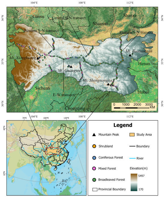
Figure 1.
Location of the study area and distribution of sample plots.
2.2. Data Processing
2.2.1. Calculation of AGB in Sample Plots
Data were collected through field surveys, which encompassed four sampling transects (three north–south lines and one east–west line) and four representative mountains (Mt. Baotianman, Mt. Shengnongjia, Mt. Guangwu, and Mt. Xionghuang). A total of 329 sample plots (400 m2 each) were established across the area, all well preserved, with minimal anthropogenic disturbance. Sampling intervals between plots on the mountains exceeded 1 km, while those along transects exceeded 5 km. Each plot’s geographical coordinates (latitude and longitude), elevation, and vegetation parameters, including species composition and ecological metrics for both tree and shrub layers, were recorded. For each woody individual, the diameter at breast height (DBH) was measured using a diameter tape, and the tree height was measured with a telescopic height pole or a laser hypsometer, depending on the tree size and site conditions. All field measurements were conducted in accordance with standardized protocols specified in national forest inventory guidelines [47].
In order to improve accuracy and minimize estimation errors, species-specific allometric equations were applied to calculate aboveground biomass (AGB) [48]. AGB values were standardized to kilograms. Initial surveys recorded 821 species, but only those with >3 individuals per species were retained, yielding a final dataset of 507 species. Allometric equations were selected based on three criteria, including high correlation coefficients, derivation from studies in provinces within or adjacent to the study region, and prioritization of genus-specific or morphologically similar species equations, when species-specific ones were unavailable. Generalized functional group equations (e.g., deciduous shrubs, evergreen shrubs, hard/soft broadleaf species) were applied for species lacking genus-specific equations; some of these generalized equations are listed in Table 1. The allometric biomass equations proposed by previous documents [49,50,51,52,53,54,55] (Table S1) were adopted following an extensive literature review. Total plot-level AGB was calculated as the sum of individual plant biomass values, categorized into broadleaf and coniferous species AGB. All values were standardized to Mg/ha for analysis.

Table 1.
Selected generalized allometric growth equations.
2.2.2. Interaction Test Between Allometric Equation Parameters and Elevation
To assess whether elevation influences the coefficients of allometric equations, a linear regression approach incorporating interaction terms was applied. This method enables testing the stability of model parameters along an elevation gradient. A random sampling strategy was used to select 20 species from those with more than 300 individuals, and their allometric equations were examined for interaction effects; these species accounted for approximately 32% of the total vegetation recorded across all sample plots.
Taking the commonly used allometric equation as an example,
By applying logarithmic transformation, the model can be expressed in linear form as
To test whether the coefficients and are affected by elevation, elevation and its interaction with the main predictor variable were introduced into the model, resulting in the following regression form:
In this model, reflects the exponent , while relates to the intercept . The significance of the coefficients and indicates whether the intercept and slope vary with elevation, respectively.
This approach is based on standard interaction modeling in ecological statistics, commonly used to examine whether environmental gradients affect species traits or functional relationships [56,57]. It allows for explicit hypothesis testing on parameter invariance without the necessity of data partitioning or predictive accuracy evaluation. The results showed that, for all randomly selected vegetation species, the coefficients of the allometric equations exhibited no significant relationship with elevation (Figure S1, Table S2).
2.2.3. Forest Type Classification
The 329 vegetation sampling plots were classified into four forest types: broadleaf forest, coniferous forest, shrubland, and mixed coniferous–broadleaf forest. This classification was based on the relative proportions of broadleaf, coniferous, and shrub species recorded within each plot, following the 2010 National Forest Resources Classification Standard of China [58]. Specifically, plots were classified as broadleaf forest if broadleaf species accounted for more than 65% of the total recorded individuals, coniferous forest if coniferous species exceeded 65%, and shrubland if shrub species exceeded 65%. For plots where none of the three groups surpassed the 65% threshold, they were categorized as mixed coniferous–broadleaf forest (as shown in Table 2).
Table 2.
Classification of forest types by proportions of tree species.
2.2.4. Outlier Detection
Cook’s distance is a widely used regression diagnostic tool for identifying influential observations that may unduly affect model estimates [59]. It measures the effect of removing a single observation from the dataset on the estimated regression coefficients. Observations with high Cook’s distance values (commonly, values larger than 4/n, where n is the number of observations) are considered influential and may be treated as outliers [60,61]. The formula for Cook’s distance is given by
where is the residual of the th observation, is the number of parameters in the model (including the intercept), the mean squared error () is the average of the squared residuals, and is the leverage value for the th observation, reflecting its influence on the regression fit.
2.3. Data Analysis
Generalized additive models (GAMs) are distinguished by their flexibility in modeling potential nonlinear relationships between response variables and predictors [62]. Unlike traditional linear models, GAMs use smooth functions (e.g., splines) to fit data, enabling the identification and description of complex relationships without requiring pre-specified functional forms [63]. In this study, the relationship between forest AGB and elevation at the plot scale was modeled using GAMs, implemented through the mgcv package (version 1.9-1) within the R statistical environment (version 4.4.1, R-Foundation for Statistical Computing, Vienna, Austria). A cubic spline was used as the smooth term to capture the nonlinear relationship between elevation and AGB density. The significance of the smooth term was assessed using ANOVA, and the model’s fit was evaluated using R2. Predicted AGB values were calculated, with 95% confidence intervals established based on standard errors.
3. Results
3.1. GAMs Analysis of AGB and Elevation Relationships Across Forest Types
After removing outliers from the data (Figure S2), the results of the quantitative classification, presented in Table 3, revealed significant differences in the average aboveground biomass (AGB) and the elevation distribution across forest types. Shrubland was observed at the lowest average elevation (1047 m), while coniferous forests were distributed at the highest average elevation (1624 m). Broadleaf forests exhibited the highest average AGB (159.67 Mg/ha), exceeding the average biomass of broadleaf forests in eastern China (142.32 Mg/ha) [64]. Similarly, the average AGB of coniferous forests (155.19 Mg/ha) was higher than that of coniferous forests in eastern China (132.78 Mg/ha) [64]. In contrast, shrubland forests had the lowest average AGB (39.48 Mg/ha), significantly lower than that of tree-dominated forests (broadleaf, coniferous, and mixed coniferous–broadleaf forests).
Table 3.
Statistical results of four forest types, their AGB values, and GAMs test after outlier removal.
The GAMs fitting results, illustrated in Table 3, indicated that the effective degrees of freedom (Edf) for broadleaf forests and shrubland were 5.84 and 5.02, respectively; both values exceeded 1 but remained below the maximum degrees of freedom (K = 9), suggesting strong nonlinear patterns without overfitting. Conversely, the Edf values for coniferous and mixed coniferous–broadleaf forests were 2.21 and 2.14, respectively, close to 1, indicating a more linear relationship between AGB and elevation. Broadleaf forest AGB displayed a distinct unimodal pattern (R2 = 0.4, p < 0.001; Figure 2a), peaking at 597.5 Mg/ha in the Mt. Shennongjia plot at 1716 m and declining above 1800 m. Coniferous forest AGB (R2 = 0.64, p < 0.001; Figure 2b) and mixed coniferous–broadleaf forest AGB (R2 = 0.46, p < 0.001; Figure 2c) increased with elevation. Shrubland AGB (R2 = 0.45, p < 0.05; Figure 2d) also increased with elevation, showing a sharp rise at 2050 m. Overall, the p-values for the significance tests of AGB across all four forest types were below 0.05, confirming that elevation significantly influences AGB.
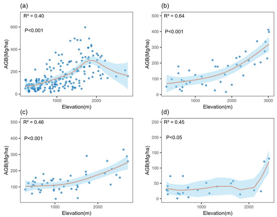
Figure 2.
Relationship between elevation and distinct forest types after outlier removal, that is, (a) broadleaf forests AGB, (b) coniferous forests AGB, (c) mixed coniferous–broadleaf forests AGB, and (d) shrubland AGB.
3.2. GAMs Analysis of AGB and Elevation Relationships Across Four Sampling Transects
In this study, outlier removal was performed only at the forest type level. No outlier detection or exclusion was applied to AGB data at the regional level. This decision was based on the relatively small sample sizes within individual regions, where the removal of even a few data points could significantly alter the observed AGB–elevation relationship. By retaining all regional data points, we aimed to preserve potential ecological gradients and avoid bias introduced by excessive data filtering. This approach ensured the integrity of subsequent analyses involving regional variation along elevation.
On the eastern S-N transect, tAGB, bAGB, and cAGB exhibited an overall increasing trend with elevation. Both tAGB (R2 = 0.65, p < 0.001; Figure 3a) and bAGB (R2 = 0.61, p < 0.001; Figure 3a) displayed a steady increase with elevation, reaching their peaks at 1795 m. cAGB did not show a significant relationship with elevation (p = 0.13; Figure 3a), indicating that elevation might not be a key factor influencing its distribution. Moreover, the Edf values for the three AGB types in the eastern S-N transect ranged between 1 and the degrees of freedom (K = 9), suggesting a nonlinear association with elevation.
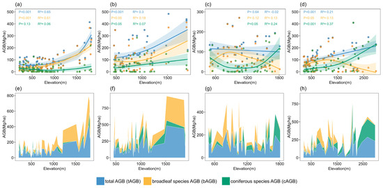
Figure 3.
Relationship between elevation and AGB components of four sampling transect plots: (a) eastern S-N transect plots, (b) central S-N transect plots, (c) western S-N transect plots, and (d) E-W transect plots. Elevational variation in AGB component accumulation within the four sampling transect plots: (e) eastern S-N transect plots, (f) central S-N transect plots, (g) western S-N transect plots, and (h) E-W transect plots.
On the central S-N transect, the three forest AGB components exhibited significant positive correlations with elevation, though the strength of these relationships differed. The R2 values for tAGB (R2 = 0.3, p < 0.001; Figure 3b) and bAGB (R2 = 0.18, p < 0.05; Figure 3b) were modest, whereas cAGB had an R2 value of 0.07, suggesting that elevation accounted for merely 7% of the forest AGB variability.
On the western S-N transect, tAGB did not show a significant relationship with elevation (p = 0.64; Figure 3c), and the low R2 value (R2 = −0.02; Figure 3c) indicated a weak model fit. Similarly, bAGB did not exhibit a significant relationship with elevation (p = 0.12; Figure 3c), and the model’s explanatory capacity was limited (R2 = 0.1; Figure 3c). In contrast, cAGB demonstrated a stronger relationship with elevation (R2 = 0.24, p < 0.05; Figure 3c), exhibiting a clear U-shaped pattern, with higher values at low and high elevations and lower values at mid elevations.
Along the E-W transect, the three forest AGB components exhibited significant associations with elevation (p < 0.05; Figure 3d). While tAGB (R2 = 0.21; Figure 3d) and cAGB (R2 = 0.37; Figure 3d) demonstrated modest explanatory capacity, both displayed an overall upward trend with elevation. In contrast, bAGB (R2 = 0.13; Figure 3d) showed the weakest explanatory capacity but exhibited a distinct unimodal distribution pattern ecologically divergent from the elevation-related trends observed in tAGB and cAGB.
In summary, the distribution patterns of forest AGB components along elevation gradients displayed notable spatial variability. The maximum values of tAGB and bAGB were predominantly found in mid-to-high elevation ranges (1300–1900 m), cAGB was relatively low in the eastern transect (Table 4), while it showed a marked increase in the central and transverse transects (Figure 3f,h), accounting for over 80% of the total AGB at elevations above 1800 m. The western S-N transect, characterized by the highest average elevation and complex topography (Figure 1, Table 4), exhibited a fragmented distribution of AGB components, with tAGB and bAGB lacking distinct elevation-dependent patterns.
Table 4.
Statistical results of four sampling transects, their AGB values, and GAM test results.
3.3. GAM Analysis of AGB and Elevation Relationships Across Four Representative Mountains
In the Mt. Baotianman plots, both tAGB (p < 0.05, R2 = 0.37; Figure 4a) and bAGB (p < 0.05, R2 = 0.35; Figure 4a) demonstrated significant relationships with elevation, displaying a unimodal distribution pattern that peaked at 1636 m. cAGB did not show a significant relationship with elevation (p < 0.1, p > 0.05, R2 = 0.1; Figure 4a), exhibiting limited explanatory capacity and a low average cAGB value.
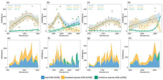
Figure 4.
Relationship between elevation and AGB components of four representative mountain plots: (a) Mt. Baotianman plots; (b) Mt. Shengnongjia plots; (c) Mt. Guangwu plots; and (d) Mt. Xionghuang plots. Elevational variation in AGB component accumulation within four representative mountain plots: (e) Mt. Baotianman plots; (f) Mt. Shengnongjia plots; (g) Mt. Guangwu plots; and (h) the Mt. Xionghuang transect plots.
In the Mt. Shengnongjia plots, the relationships between all three forest AGB components and elevation were significant (p < 0.001; Figure 4b), demonstrating strong explanatory capacity. tAGB displayed a bimodal distribution with elevation, reaching a peak at 1922 m, decreasing afterward, and then increasing again at 2500 m. bAGB exhibited a unimodal distribution pattern with elevation, with its peak also occurring at 1922 m. cAGB demonstrated a significant positive correlation with elevation (p < 0.001, R2 = 0.4; Figure 4b), characterized by a monotonically increasing linear trend.
In the Mt. Guangwu plots, both tAGB (p < 0.05, R2 = 0.39; Figure 4c) and bAGB (p < 0.05, R2 = 0.37; Figure 4c) exhibited significant relationships with elevation, displaying a unimodal distribution pattern that peaked at 2022 m; cAGB showed a near-significant relationship with elevation (p < 0.1, p > 0.05, R2 = 0.11; Figure 4c), holding limited ecological relevance, and the average coniferous AGB was notably low at 4.8 Mg/ha.
In the Mt. Xionghuang plots, tAGB exhibited a near-significant relationship with elevation (p < 0.1, p > 0.05; Figure 4d), though the model’s explanatory capacity is limited (R2 = 0.22; Figure 4d). bAGB did not show a significant relationship with elevation (p = 0.25; Figure 4d), and the model’s explanatory capacity remains modest (R2 = 0.25; Figure 4d). In contrast, cAGB demonstrated a highly significant relationship with elevation (p < 0.001; Figure 4d), with exceptionally high model explanatory capacity (R2 = 0.98; Figure 4d), suggesting that elevation is a strong predictor of cAGB distribution, particularly at elevations above 2750 m, where cAGB growth rates markedly increase.
The results showed that tAGB, bAGB, and cAGB exhibit significant variation along the altitudinal gradient in the same sampling plots (Figure 4). The peaks of tAGB and bAGB were observed between 1600 and 2800 m, with the highest peak elevation found in the Mt. Xionghuang plots (2800 m) and the lowest in the Mt. Baotianman plots (1650 m). bAGB was predominant in low-elevation areas (>70%). In the Mt. Guangwu plots, the cAGB content was relatively low and showed no distinct distribution pattern, while in the Mt. Baotianman, Mt. Shengnongjia, and Mt. Xionghuang plots, cAGB progressively increased at higher elevations, with sharp rises at 1740 m, 2049 m, and 2900 m, respectively, and overall proportions surpassing 50% (Figure 4e,f,h).
In general, the forest AGB in the four representative mountains showed a significant relationship with elevation, with greater explanatory capacity than that observed along the four sampling transects. Moreover, the mountain AGB of the four representative mountains was higher than that of the four sampling transects (Table 4).
4. Discussion
Research on AGB in the Qinling–Daba Mountains region is limited, with most studies focusing on single areas and single community types. Yao et al. [65] analyzed the horizontal distribution patterns of broadleaf forest AGB and studied the effects of four factors (e.g., topography, temperature, precipitation, and human activities) on broadleaf forest AGB. The results indicated that topography is the second-most influential factor for broadleaf forest AGB after temperature, which aligns with this study’s conclusion that elevation significantly affects forest AGB. One study [66] reported that stand age significantly affects the AGB of Quercus variabilis, with AGB gradually decreasing as stand age increases. However, the study did not consider the influence of elevation. Another study [67] conducted in Huoditang, Qinling Mountains, estimated the average AGB of Q. aliena var. acuteserrata forests at 259.24 Mg/ha, which is higher than the 159.67 Mg/ha average for broadleaf forests in this study. Similarly, the average AGB of Pinus armandi forests is 174.38 Mg/ha, exceeding the 155.19 Mg/ha recorded for coniferous forests in this study. Mixed forests have an average AGB of 188.5 Mg/ha, also higher than the 136.55 Mg/ha observed in mixed coniferous–broadleaf forests in this study. However, this study did not investigate the factors influencing forest AGB.
4.1. Effect of Elevation Gradient on the AGB of Different Forest Types
The results revealed significant differences in the AGB distribution across forest types and elevation zones. Broadleaf forest AGB exhibited a unimodal distribution along the elevational gradient (Figure 2b), peaking at mid-elevation zones around 1716 m. Above 1800 m, broadleaf forest AGB declined, suggesting that photosynthetic activities of dominant species, such as Quercus variabilis Blume and Quercus acutissima Carruth, are inhibited by low temperatures at high elevations [68]. Combined with poor soil conditions and colder climates at higher altitudes, these factors collectively constrain broadleaf tree growth and reduce AGB [69]. Notably, 1800 m remains within the elevational distribution range of broadleaf forests in the Qinling–Daba Mountains [45]. Coniferous forest AGB increased with elevation (Figure 2b), aligning with elevational carbon storage trends in subalpine coniferous forests in New Mexico, USA [30]. This reflects the adaptive capacity of coniferous species to thrive under low temperatures and nutrient-poor soils, enabling their dominance at higher elevations [70,71]. Mixed coniferous–broadleaf forests showed increasing AGB with elevation (Figure 2c), possibly driven by microclimatic variation, which, in turn, modified interspecific competition [72]. At mid-to-low elevations (300–1800 m), AGB allocation exhibited intense competition between broadleaf and coniferous species. Above 1800 m, however, coniferous species demonstrated enhanced adaptability to environmental stressors, such as low temperatures, strong winds, and shorter growing seasons, tilting competitive advantages toward coniferous growth and elevating overall AGB [73]. Nevertheless, research on mixed forests remains scarce, particularly regarding high-elevation biomass dynamics and competition mechanisms. Existing studies predominantly focus on pure broadleaf or coniferous forests, leaving the elevational patterns and underlying mechanisms of mixed forest AGB underexplored.
This study also identified a marked increase in shrubland AGB at high elevations (>2100 m) (Figure 2d), a phenomenon reported in other mountain ecosystems. This observed pattern highlights shrubs’ enhanced cold tolerance and growth adaptability in high-elevation environments compared to arborescent species, corresponding to a study in the Hengduan Mountains, China, with shrubs becoming nearly exclusive at extreme elevations [74]. However, these findings contrast with observations on Mount Kilimanjaro, Africa [75]. Potential explanations of the discrepancy may primarily stem from climatic divergence between the study regions, combined with the distinct adaptive strategies of dominant shrub species. Specifically, key high-elevation species, such as Rosa omeiensi Rolfe and Viburnum sympodiale Graebn exhibit cold tolerance, shade adaptation, and low soil requirements in the Qinling–Daba Mountains, which is a temperate–subtropical transition zone in China.
4.2. Elevational AGB Patterns Corresponding to the Mid-Domain Effect
Significant variations in AGB distribution patterns were observed across sampling regions, confirming the mid-domain effect [76,77]. Most areas exhibited unimodal distributions for tAGB and bAGB, with peaks typically occurring at mid elevations, such as bAGB in the E-W transect (1300 m) (Figure 3d) and tAGB and bAGB in Mt. Baotianman (1500 m) (Figure 4a), Mt. Shengnongjia (1800 m) (Figure 4b), and Mt. Guangwu (2000 m) (Figure 4c) plots. In contrast, Mt. Xionghuang displayed a unique bimodal bAGB distribution (2050 m and 2600 m) (Figure 4d). These regions spanned large elevation ranges, exceeding 1000 m and, in some cases, 2000 m; such large elevation spans often lead to distinct vegetation distribution patterns [78]. In mountain systems, elevation indirectly regulates the plant community composition by influencing water availability and temperature redistribution [79,80]. Environmental constraints at low and high elevations contrast with the more favorable hydrothermal conditions at mid elevations, with typical bAGB peaks. This finding enriches the mid-domain effect by incorporating biomass perspectives.
On the eastern S-N and central S-N transects (Figure 3a), tAGB and bAGB did not exhibit unimodal or bimodal trends but instead showed monotonically increasing patterns. This is attributed to the relatively low average elevation of the eastern S-N transect (756 m) and central S-N transect (883 m) in the Qinling–Daba Mountains, where sampling plots were concentrated in the low-to-mid elevation range (200–1200 m), with the highest sampling plots not exceeding 1900 m. Stacked plots (Figure 3a) revealed that tAGB along these transects was primarily contributed by bAGB, and the elevation range remained within the suitable growth interval for broadleaf forests, explaining the monotonically increasing trend. In contrast, tAGB (p = 0.64, R2 = −0.02; Figure 3c) and bAGB (p = 0.12, R2 = 0.13; Figure 3c) in the western S-N transect plots showed no significant correlation with elevation.
4.3. Component-Specific Responses of Forest AGB to Elevational Gradients
This study revealed component-specific responses of forest AGB to elevational gradients at the plot scale (Figure 3 and Figure 4). Despite consistent geographical conditions across the study area, distinct heterogeneities were observed in the elevational distribution patterns of the total AGB (tAGB), broadleaf species AGB (bAGB), and coniferous species AGB (cAGB). For instance, within the E-W transect (Figure 3a), tAGB and cAGB exhibited positive correlations with elevation, whereas bAGB followed a unimodal distribution, initially increasing and then decreasing with elevation. This divergence likely reflects the dominance of broadleaf species in mid-elevation monospecific communities [68] and the competitive advantage of coniferous species at higher elevations [30]. In the Mt. Shengnongjia plots (Figure 4b), tAGB displayed a bimodal distribution along the elevational gradient, contrasting with the unimodal pattern of bAGB and the linear positive correlation of cAGB (Edf = 1; Table 4). These elevational response characteristics in the AGB composition align with reports on Mt. Shengnongjia [81]. Notably, cAGB in the Mt. Xionghuang plots demonstrated strong elevational dependency (R2 = 0.98; Figure 4d), potentially indicating high-elevation adaptation of coniferous species to cold environments [82], which restricts their spatial distribution to specific elevational thresholds, with more than 50% cAGB contributing above 2900 m (Figure 4h) [83].
Highlighting the critical influence of the research scale on elevation–AGB interpretations, the findings demonstrated pronounced variability across observational contexts. The low explanatory capacity observed in sampling transect plots, for instance, tAGB R2 = −0.02 in the western S-N transect (Figure 3c), likely originates from environmental heterogeneity, including soil types, anthropogenic disturbance gradients, and topographic complexity. In contrast, the strong model fit for representative mountain plots, particularly R2 = 0.69 in Mt. Shengnongjia plots, suggests that small-scale studies better capture elevation-driven ecological processes. These findings offer implications for integrated forest management. The AGB dominance of coniferous species at high elevations, such as more than 80% cAGB contributing above 2600 m in Mt. Shengnongjia plots and over 50% cAGB contributing above 2900 m in Mt. Xionghuang plots (Figure 4f,h), may indicate these areas as frontline zones for treeline shifts under global warming [84,85]. Additionally, regions with narrow elevational niches for cAGB, specifically those above 2750 m in Mt. Xionghuang plots (Figure 4h), require prioritized monitoring to prevent abrupt declines in ecosystem services [86].
However, this study has limitations. Firstly, although the methods were effective for isolating elevation-driven processes, the plot-scale focus weakens the explanatory capacity for cross-regional AGB–elevation patterns (e.g., the western S-N transect). Secondly, the significant increase in shrubland AGB at high elevations lacks mechanistic clarity from species adaptability and interspecific competition, and discrepancies with tropical studies remain unresolved. Thirdly, although elevation significantly influences forest AGB, its low explanatory capacity underscores the need to incorporate additional factors, such as soil properties, moisture, and temperature, for comprehensive interpretation.
5. Conclusions
This study examined variations in AGB along elevation gradients across different forest types in the Qinling–Daba Mountains, using data from 329 vegetation survey plots. Broadleaf forest AGB peaks at mid elevations (597.5 Mg/ha) and declines with increasing elevation (p < 0.001). In contrast, coniferous and mixed forests show increasing AGB with elevation (p < 0.001), indicating different response patterns. Shrubland AGB remains lower than that in forested areas but increases above 2050 m (p < 0.05).
AGB component responses to elevation also vary. In the sampling transects, tAGB and bAGB peak between 1300 and 1900 m, while the cAGB proportion significantly increases above 1800 m, reaching over 80% at its peak. In representative mountainous regions, tAGB and bAGB show unimodal distributions, whereas cAGB peaks at higher elevations. Compared to large-scale transects, areas with complex microtopography demonstrate greater sensitivity to elevation, highlighting the amplification of environmental effects in heterogeneous terrains.
This study emphasizes the critical role of elevation in shaping forest AGB distribution in the Qinling–Daba Mountains and reveals the complex relationship between AGB and elevation gradients, offering insights into montane forest carbon storage and ecological mechanisms. In mid-elevation zones, broadleaf species should be protected from excessive disturbance or logging to maintain their high AGB levels, while at higher elevations, conservation efforts should focus on coniferous and shrub species to prevent the upward shift of the treeline.
Supplementary Materials
The following supporting information can be downloaded at: https://www.mdpi.com/article/10.3390/f16050796/s1, Table S1: Allometric growth equation of species (number > 3); Table S2: Effects of elevation on the stability of species-specific allometric coefficients evaluated via interaction models; Figure S1: Effects of elevation on the stability of species-specific allometric coefficients evaluated via interaction models; Figure S2: Outlier identification based on the Cook’s distance method.
Author Contributions
Conceptualization, Y.H.; methodology, Y.H., D.L. and X.Y.; software, Y.H.; validation, Y.H.; formal analysis, Y.H.; investigation, B.Z.; resources, B.Z.; data curation, Y.H.; writing—original draft, Y.H.; writing—review and editing, W.Z. and X.Y.; visualization, Y.H.; supervision, W.Z.; project administration, W.Z.; funding acquisition, W.Z. All authors have read and agreed to the published version of the manuscript.
Funding
This research received no external funding.
Data Availability Statement
The data presented in this study are available on request from the corresponding author.
Conflicts of Interest
The authors declare no conflicts of interest.
References
- Dixon, R.K.; Brown, S.; Houghton, R.A.; Solomon, A.M.; Trexler, M.C.; Wisniewski, J. Carbon pools and flux of global forest ecosystems. Science 1994, 265, 185–190. [Google Scholar] [CrossRef] [PubMed]
- Pan, Y.; Birdsey, R.A.; Phillips, O.L.; Houghton, R.A.; Fang, J.; Kauppi, P.E.; Keith, H.; Kurz, W.A.; Ito, A.; Lewis, S.L.; et al. The enduring world forest carbon sink. Nature 2024, 631, 563–569. [Google Scholar] [CrossRef] [PubMed]
- Kolomyts, E.G. Predictive modelling of boreal forest resources in regulation of the carbon cycle and mitigation of the global warming. Int. J. Glob. Warm. 2022, 27, 333–364. [Google Scholar] [CrossRef]
- Zhao, J.; Hu, H.; Wang, J. Forest carbon reserve calculation and comprehensive economic value evaluation: A forest management model based on both biomass expansion factor method and total forest value. Int. J. Environ. Res. Public Health 2022, 19, 15925. [Google Scholar] [CrossRef]
- Saatchi, S.S.; Harris, N.L.; Brown, S.; Lefsky, M.; Mitchard, E.T.A.; Salas, W.; Zutta, B.R.; Buermann, W.; Lewis, S.L.; Hagen, S.; et al. Benchmark map of forest carbon stocks in tropical regions across three continents. Proc. Natl. Acad. Sci. USA 2011, 108, 9899–9904. [Google Scholar] [CrossRef]
- Austin, K.G.; Baker, J.S.; Sohngen, B.L.; Wade, C.M.; Daigneault, A.; Ohrel, S.B.; Ragnauth, S.; Bean, A. The economic costs of planting, preserving, and managing the world’s forests to mitigate climate change. Nat. Commun. 2020, 11, 5946. [Google Scholar] [CrossRef]
- Fang, J.; Wang, G.; Liu, G.; Xu, S. Forest biomass of China: An estimate based on the biomass-volume relationship. Ecol. Appl. 1998, 8, 1084–1091. [Google Scholar] [CrossRef]
- Li, G.; Zhou, G.; Wang, X.; Wu, Z.; Qiu, Z.; Zhao, H.; Liang, R. Aboveground biomass of natural Castanopsis fissa community at the Xiaokeng of NanLing Mountain, Southern China. Acta Ecol. Sin. 2011, 31, 3650–3658. [Google Scholar]
- Fang, J.; Chen, A.; Peng, C.; Zhao, S.; Ci, L. Changes in forest biomass carbon storage in China between 1949 and 1998. Science 2001, 292, 2320–2322. [Google Scholar] [CrossRef]
- Fang, J.Y.; Wang, Z.M. Forest biomass estimation at regional and global levels, with special reference to China’s forest biomass. Ecol. Res. 2001, 16, 587–592. [Google Scholar] [CrossRef]
- Swoish, M.; Leme Filho, J.F.D.C.; Reiter, M.S.; Campbell, J.B.; Thomason, W.E. Comparing satellites and vegetation indices for cover crop biomass estimation. Comput. Electron. Agric. 2022, 196, 106900. [Google Scholar] [CrossRef]
- Silva, C.A.; Duncanson, L.; Hancock, S.; Neuenschwander, A.; Thomas, N.; Hofton, M.; Fatoyinbo, L.; Simard, M.; Marshak, C.Z.; Armston, J.; et al. Fusing simulated GEDI, ICESat-2 and NISAR data for regional aboveground biomass mapping. Remote Sens. Environ. 2021, 253, 112234. [Google Scholar] [CrossRef]
- Navarro, A.; Young, M.; Allan, B.; Carnell, P.; Macreadie, P.; Ierodiaconou, D. The application of Unmanned Aerial Vehicles (UAVs) to estimate above-ground biomass of mangrove ecosystems. Remote Sens. Environ. 2020, 242, 111747. [Google Scholar] [CrossRef]
- Alvarez, E.; Duque, A.; Saldarriaga, J.; Cabrera, K.; de Las Salas, G.; del Valle, I.; Lema, A.; Moreno, F.; Orrego, S.; Rodriguez, L. Tree above-ground biomass allometries for carbon stocks estimation in the natural forests of Colombia. For. Ecol. Manag. 2012, 267, 297–308. [Google Scholar] [CrossRef]
- Razaq, M.; Huang, Q.; Wang, F.; Liu, C.; Gnanamoorthy, P.; Liu, C.; Tang, J. Carbon stock dynamics in rubber plantations along an elevational gradient in tropical China. Forests 2024, 15, 1933. [Google Scholar] [CrossRef]
- Asner, G.P.; Hughes, R.F.; Varga, T.A.; Knapp, D.E.; Kennedy-Bowdoin, T. Environmental and biotic controls over aboveground biomass throughout a tropical rain forest. Ecosystems 2009, 12, 261–278. [Google Scholar] [CrossRef]
- Bunker, D.E.; DeClerck, F.; Bradford, J.C.; Colwell, R.K.; Perfecto, I.; Phillips, O.L.; Sankaran, M.; Naeem, S. Species loss and aboveground carbon storage in a tropical forest. Science 2005, 310, 1029–1031. [Google Scholar] [CrossRef]
- Slik, J.W.F.; Paoli, G.; McGuire, K.; Amaral, I.; Barroso, J.; Bastian, M.; Blanc, L.; Bongers, F.; Boundja, P.; Clark, C.; et al. Large trees drive forest aboveground biomass variation in moist lowland forests across the tropics. Glob. Ecol. Biogeogr. 2013, 22, 1261–1271. [Google Scholar] [CrossRef]
- Chen, C.; Xiao, W.; Chen, H.Y.H. Meta-analysis reveals global variations in plant diversity effects on productivity. Nature 2025, 638, 435–440. [Google Scholar] [CrossRef]
- Pugh, T.A.M.; Arneth, A.; Kautz, M.; Poulter, B.; Smith, B. Important role of forest disturbances in the global biomass turnover and carbon sinks. Nat. Geosci. 2019, 12, 730. [Google Scholar] [CrossRef]
- DeWalt, S.J.; Chave, J. Structure and biomass of four lowland neotropical forests. Biotropica 2004, 36, 7–19. [Google Scholar] [CrossRef]
- Dyderski, M.K.; Pawlik, Ł. Drivers of forest aboveground biomass and its increments in the Tatra Mountains after 15 years. Catena 2021, 205, 105468. [Google Scholar] [CrossRef]
- Liu, L.; Zeng, F.; Song, T.; Wang, K.; Du, H. Stand structure and abiotic factors modulate karst forest biomass in southwest China. Forests 2020, 11, 443. [Google Scholar] [CrossRef]
- Chen, Y.; Zhang, S.; Wang, Y. Spatial distribution patterns and drivers of above- and below-biomass in Chinese terrestrial ecosystems. Sci. Total Environ. 2024, 944, 173922. [Google Scholar] [CrossRef]
- Riihimäki, H.; Heiskanen, J.; Luoto, M. The effect of topography on arctic-alpine aboveground biomass and NDVI patterns. Int. J. Appl. Earth Obs. Geoinf. 2017, 56, 44–53. [Google Scholar] [CrossRef]
- Sandoya, V.; Saura-Mas, S.; Granzow-de la Cerda, I.; Arellano, G.; Macía, M.J.; Tello, J.S.; Lloret, F. Contribution of species abundance and frequency to aboveground forest biomass along an Andean elevation gradient. For. Ecol. Manag. 2021, 479, 118549. [Google Scholar] [CrossRef]
- Cuni-Sanchez, A.; Sullivan, M.J.P.; Platts, P.J.; Lewis, S.L.; Marchant, R.; Imani, G.; Hubau, W.; Abiem, I.; Adhikari, H.; Albrecht, T.; et al. High aboveground carbon stock of African tropical montane forests. Nature 2021, 596, 536–542. [Google Scholar] [CrossRef]
- Moser, G.; Leuschner, C.; Hertel, D.; Graefe, S.; Soethe, N.; Iost, S. Elevation effects on the carbon budget of tropical mountain forests (S Ecuador): The role of the belowground compartment. Glob. Change Biol. 2011, 17, 2211–2226. [Google Scholar] [CrossRef]
- Bai, J.; Long, C.; Quan, X.; Liao, C.; Zhai, D.; Bao, Y.; Men, X.; Zhang, D.; Cheng, X. Reverse diversity–biomass patterns in grasslands are constrained by climates and stoichiometry along an elevational gradient. Sci. Total Environ. 2024, 917, 170416. [Google Scholar] [CrossRef]
- Anderson-Teixeira, K.J.; Delong, J.P.; Fox, A.M.; Brese, D.A.; Litvak, M.E. Differential responses of production and respiration to temperature and moisture drive the carbon balance across a climatic gradient in New Mexico. Glob. Change Biol. 2011, 17, 410–424. [Google Scholar] [CrossRef]
- Hemp, A. Continuum or zonation? Altitudinal gradients in the forest vegetation of Mt. Kilimanjaro. Plant Ecol. 2006, 184, 27–42. [Google Scholar] [CrossRef]
- Fadrique, B.; Báez, S.; Duque, Á.; Malizia, A.; Blundo, C.; Carilla, J.; Osinaga-Acosta, O.; Malizia, L.; Silman, M.; Farfán-Ríos, W.; et al. Author Correction: Widespread but heterogeneous responses of Andean forests to climate change. Nature 2019, 565, E10. [Google Scholar] [CrossRef] [PubMed]
- Wang, Y.; Liu, Y.; Chen, P.; Song, J.; Fu, B. Interannual precipitation variability dominates the growth of alpine grassland above-ground biomass at high elevations on the Tibetan Plateau. Sci. Total Environ. 2024, 931, 172745. [Google Scholar] [CrossRef]
- Richardson, A.D.; Keenan, T.F.; Migliavacca, M.; Ryu, Y.; Sonnentag, O.; Toomey, M. Climate change, phenology, and phenological control of vegetation feedbacks to the climate system. Agric. For. Meteorol. 2013, 169, 156–173. [Google Scholar] [CrossRef]
- Gao, M.; Piao, S.; Chen, A.; Yang, H.; Liu, Q.; Fu, Y.H.; Janssens, I.A. Divergent changes in the elevational gradient of vegetation activities over the last 30 years. Nat. Commun. 2019, 10, 2970. [Google Scholar] [CrossRef]
- Tao, J.; Zhang, Y.; Dong, J.; Fu, Y.; Zhu, J.; Zhang, G.; Jiang, Y.; Tian, L.; Zhang, X.; Zhang, T.; et al. Elevation-dependent relationships between climate change and grassland vegetation variation across the Qinghai-Xizang Plateau. Int. J. Climatol. 2015, 35, 1638–1647. [Google Scholar] [CrossRef]
- Zhang, S.; Xu, H.; Liu, A.; Qi, S.; Hu, B.; Huang, M.; Luo, J. Mapping of secondary forest age in China using stacked generalization and Landsat time series. Sci. Data 2024, 11, 302. [Google Scholar] [CrossRef]
- Wei, X.; Liu, R.; Liu, Y.; He, J.; Chen, J.; Qi, L.; Zhou, Y.; Qin, Y.; Wu, C.; Dong, J.; et al. Forest Areas in China Are Recovering Since the 21st Century. Geophys. Res. Lett. 2024, 51, e2024GL110312. [Google Scholar] [CrossRef]
- Xia, X.; Xia, J.; Chen, X.; Fan, L.; Liu, S.; Qin, Y.; Qin, Z.; Xiao, X.; Xu, W.; Yue, C.; et al. Reconstructing Long-Term Forest Cover in China by Fusing National Forest Inventory and 20 Land Use and Land Cover Data Sets. J. Geophys. Res. Biogeosciences 2023, 128, e2022JG007101. [Google Scholar] [CrossRef]
- Gao, H.; Fu, T.; Liu, J.; Liang, H.; Han, L. Ecosystem Services Management Based on Differentiation and Regionalization along Vertical Gradient in Taihang Mountain, China. Sustainability 2018, 10, 986. [Google Scholar] [CrossRef]
- Mi, X.; Feng, G.; Hu, Y.; Zhang, J.; Chen, L.; Corlett, R.T.; Hughes, A.C.; Pimm, S.; Schmid, B.; Shi, S.; et al. The global significance of biodiversity science in China: An overview. Natl. Sci. Rev. 2021, 8, nwab032. [Google Scholar] [CrossRef] [PubMed]
- Zhang, L.; Song, C.; Yan, J. Spatio-temporal trends of annual extreme temperature in northern and southern qinling mountains. Sci. Geogr. Sin. 2011, 31, 1007–1011. [Google Scholar]
- Zhang, B. Ten major scientific issues concerning the study of China’s north-south transitional zone. Prog. Geogr. 2019, 38, 305–311. [Google Scholar] [CrossRef]
- Cheng, Y.; Huo, A.; Liu, F.; Ahmed, A.; Abuarab, M.E.; Elbeltagi, A.; Kucher, D.E. Spatiotemporal Variation of Soil Erosion in the Northern Foothills of the Qinling Mountains Using the RUSLE Model. Water 2024, 16, 2187. [Google Scholar] [CrossRef]
- Li, J.; Yao, Y.; Liu, J.; Zhang, B. Variation Analysis of the Typical Altitudinal Belt Width in the Qinling–Daba Mountains. Nat. Prot. Areas 2023, 3, 12–25. [Google Scholar] [CrossRef]
- Zhang, B.; Yao, Y.; Xiao, F.; Zhou, W.; Zhu, L.; Zhang, J.; Zhao, F.; Bai, H.; Wang, J.; Yu, F.; et al. The finding and significance of the super altitudinal belt of montane deciduous broad-leaved forests in central Qinling Mountains. Acta Geogr. Sin. 2022, 77, 2236–2248. [Google Scholar] [CrossRef]
- GB/T 26424-2010; Technical Regulations for Inventory for Forest Management Planning and Design. Institute of Forest Ecological Environment and Protection, Chinese Academy of Forestry Sciences: Beijing, China, 2011; pp. 1–3.
- Molto, Q.; Rossi, V.; Blanc, L. Error propagation in biomass estimation in tropical forests. Methods Ecol. Evol. 2013, 4, 175–183. [Google Scholar] [CrossRef]
- GB/T 43648-2024; Tree Biomass Models and Related Parameters to Carbon Accounting for Major Tree Species. National Forestry and Grassland Administration Forest and Grassland Survey and Planning Institute: Beijing, China, 2024; pp. 5–8.
- Xie, Z. Manual of Biomass Models for Common Shrubs in China; Longmen Bookstore: Beijing, China, 2018; pp. 78–139. [Google Scholar]
- Luo, Y.; Wang, X.; Ouyang, Z.; Lu, F.; Feng, L.; Tao, J. A review of biomass equations for China’s tree species. Earth Syst. Sci. Data 2020, 12, 21–40. [Google Scholar] [CrossRef]
- Li, H.; Lei, Y. Assessment of Forest Vegetation Biomass and Carbon Storage in China; China Forestry Publishing House: Beijing, China, 2010; pp. 82–99. [Google Scholar]
- Conti, G.; Gorne, L.D.; Zeballos, S.R.; Lipoma, M.L.; Gatica, G.; Kowaljow, E.; Whitworth-Hulse, J.I.; Cuchietti, A.; Poca, M.; Pestoni, S.; et al. Developing allometric models to predict the individual aboveground biomass of shrubs worldwide. Glob. Ecol. Biogeogr. 2019, 28, 961–975. [Google Scholar] [CrossRef]
- Zhou, G.; Yin, G.; Tang, X. Carbon Storage of Forest Ecosystems in China: Biomass Equation; Longmen Bookstore: Beijing, China, 2018; pp. 183–192. [Google Scholar]
- Wu, J.; Zhu, J.; Ai, X.; Yao, L.; Guo, Q.; Yan, F.; Xue, W. Meta-analysis of woody plant biomass model of subtropical evergreen deciduous broadleaf mixed forests. J. Cent. South Univ. For. Technol. 2023, 43, 111–122. [Google Scholar]
- Pfennigwerth, A.A.; Bailey, J.K.; Schweitzer, J.A. Trait variation along elevation gradients in a dominant woody shrub is population-specific and driven by plasticity. AoB Plants 2017, 9, plx027. [Google Scholar] [CrossRef] [PubMed]
- Stoklosa, J.; Daly, C.; Foster, S.D.; Ashcroft, M.B.; Warton, D.I. A climate of uncertainty: Accounting for error in climate variables for species distribution models. Methods Ecol. Evol. 2015, 6, 412–423. [Google Scholar] [CrossRef]
- GB/T 14721-2010; Classification and Codes for Forestry Resources—Forest Types. Institute of Forest Ecological Environment and Protection, Chinese Academy of Forestry Sciences: Beijing, China, 2010; p. 6.
- Rahmatullah Imon, A.H.M. Identifying multiple influential observations in linear regression. J. Appl. Stat. 2005, 32, 929–946. [Google Scholar] [CrossRef]
- Alhowyan, A.; Mahdi, W.A.; Obaidullah, A.J. Computational intelligence investigations on evaluation of salicylic acid solubility in various solvents at different temperatures. Sci. Rep. 2025, 15, 7142. [Google Scholar] [CrossRef]
- Cook, R.D. Detection of Influential Observation in Linear Regression. Technometrics 1977, 19, 15–18. [Google Scholar] [CrossRef]
- Martinez, A.d.l.I.; Labib, S.M. Demystifying normalized difference vegetation index (NDVI) for greenness exposure assessments and policy interventions in urban greening. Environ. Res. 2023, 220, 115155. [Google Scholar] [CrossRef]
- Guisan, A.; Edwards, T.C.; Hastie, T. Generalized linear and generalized additive models in studies of species distributions: Setting the scene. Ecol. Model. 2002, 157, 89–100. [Google Scholar] [CrossRef]
- Gao, Y.; Liu, X.; Min, C.; He, H.; Yu, G.; Liu, M.; Zhu, X.; Wang, Q. Estimation of the North-South Transect of Eastern China forest biomass using remote sensing and forest inventory data. Int. J. Remote Sens. 2013, 34, 5598–5610. [Google Scholar] [CrossRef]
- Yao, Y. Spatial pattern of forest aboveground biomass and its environmental influencing factors in Qinling–Daba Mountains, central China. Sci. Rep. 2024, 14, 21411. [Google Scholar] [CrossRef]
- Jiang, P.; Chen, Y.; Cao, Y. C:N:P Stoichiometry and Carbon Storage in a Naturally-Regenerated Secondary Quercus variabilis Forest Age Sequence in the Qinling Mountains, China. Forests 2017, 8, 281. [Google Scholar] [CrossRef]
- Yuan, J.; Jose, S.; Zheng, X.; Cheng, F.; Hou, L.; Li, J.; Zhang, S. Dynamics of Coarse Woody Debris Characteristics in the Qinling Mountain Forests in China. Forests 2017, 8, 403. [Google Scholar] [CrossRef]
- Koerner, C. The use of ‘altitude’ in ecological research. Trends Ecol. Evol. 2007, 22, 569–574. [Google Scholar] [CrossRef] [PubMed]
- Shi, H.; Zhou, Q.; Xie, F.; He, N.; He, R.; Zhang, K.; Zhang, Q.; Dang, H. Disparity in elevational shifts of upper species limits in response to recent climate warming in the Qinling Mountains, North-central China. Sci. Total Environ. 2020, 706, 135718. [Google Scholar] [CrossRef]
- Zhang, W.; Gou, X.; Liu, W.; Li, J.; Su, J.; Dilawar, N.; Zhu, F.; Xia, J.; Du, M.; Wang, L.; et al. Divergent tree radial growth patterns of Qinghai spruce (Picea crassifolia) at the alpine timberline along a moisture gradient in the Qilian mountains, Northwest China. Agric. For. Meteorol. 2023, 328, 109240. [Google Scholar] [CrossRef]
- Hikosaka, K.; Kurokawa, H.; Arai, T.; Takayanagi, S.; Tanaka, H.O.; Nagano, S.; Nakashizuka, T. Intraspecific variations in leaf traits, productivity and resource use efficiencies in the dominant species of subalpine evergreen coniferous and deciduous broad-leaved forests along the altitudinal gradient. J. Ecol. 2021, 109, 1804–1818. [Google Scholar] [CrossRef]
- Díaz-Calafat, J.; Uria-Diez, J.; Brunet, J.; De Frenne, P.; Vangansbeke, P.; Felton, A.; Öckinger, E.; Cousins, S.A.O.; Bauhus, J.; Ponette, Q.; et al. From broadleaves to conifers: The effect of tree composition and density on understory microclimate across latitudes. Agric. For. Meteorol. 2023, 341, 109684. [Google Scholar] [CrossRef]
- Blanco-Cano, L.; Navarro-Cerrillo, R.M.; González-Moreno, P. Biotic and abiotic effects determining the resilience of conifer mountain forests: The case study of the endangered Spanish fir. For. Ecol. Manag. 2022, 520, 120356. [Google Scholar] [CrossRef]
- Tian, L.; Zhou, L.; Sun, J.; Zong, H. Spatial distribution of tree-shrub patches and their diversity along the altitude gradient in the transition zone between the first and second steps of the northern Hengduan Mountains. Acta Ecol. Sin. 2023, 43, 10320–10333. [Google Scholar]
- Ensslin, A.; Rutten, G.; Pommer, U.; Zimmermann, R.; Hemp, A.; Fischer, M. Effects of elevation and land use on the biomass of trees, shrubs and herbs at Mount Kilimanjaro. Ecosphere 2015, 6, art45. [Google Scholar] [CrossRef]
- Colwell, R.K.; Lees, D.C. The mid-domain effect: Geometric constraints on the geography of species richness. Trends Ecol. Evol. 2000, 15, 70–76. [Google Scholar] [CrossRef]
- Wang, X.; Fang, J. The mid-domain effect hypothesis: Models, evidence and limitations. Biodivers. Sci. 2009, 17, 568. [Google Scholar]
- Gebrehiwot, K.; Demissew, S.; Woldu, Z.; Fekadu, M.; Desalegn, T.; Teferi, E. Elevational changes in vascular plants richness, diversity, and distribution pattern in Abune Yosef mountain range, Northern Ethiopia. Plant Divers. 2019, 41, 220–228. [Google Scholar] [CrossRef] [PubMed]
- Zong, N.; Shi, P. Enhanced community production rather than structure improvement under nitrogen and phosphorus addition in severely degraded alpine meadows. Sustainability 2019, 11, 2023. [Google Scholar] [CrossRef]
- Dorji, T.; Moe, S.R.; Klein, J.A.; Totland, O. Plant species richness, evenness, and composition along environmental gradients in an alpine meadow grazing ecosystem in central Tibet, China. Arct. Antarct. Alp. Res. 2014, 46, 308–326. [Google Scholar] [CrossRef]
- Ma, M.; Shen, G.; Xiong, G.; Zhao, C.; Xu, W.; Zhou, Y.; Xie, Z. Characteristic and representativeness of the vertical vegetation zonation along the altitudinal gradient in Shennongjia Natural Heritage. Chin. J. Plant Ecol. 2017, 41, 1127–1139. [Google Scholar]
- Turunen, M.; Latola, K. UV-B radiation and acclimation in timberline plants. Environ. Pollut. 2005, 137, 390–403. [Google Scholar] [CrossRef]
- Yang, W.; Wang, Y.; Webb, A.A.; Li, Z.; Tian, X.; Han, Z.; Wang, S.; Yu, P. Influence of climatic and geographic factors on the spatial distribution of Qinghai spruce forests in the dryland Qilian Mountains of Northwest China. Sci. Total Environ. 2018, 612, 1007–1017. [Google Scholar] [CrossRef]
- Zhang, Y.; An, C. Satellites reveal global migration patterns of natural mountain treelines during periods of rapid warming. Forests 2024, 15, 1780. [Google Scholar] [CrossRef]
- Hansson, A.; Dargusch, P.; Shulmeister, J. A review of modern treeline migration, the factors controlling it and the implications for carbon storage. J. Mt. Sci. 2021, 18, 291–306. [Google Scholar] [CrossRef]
- Sasanifar, S.; Alijanpour, A.; Shafiei, A.B.; Rad, J.E.; Molaei, M.; Álvarez-Álvarez, P. Understanding how forest ecosystem services are affected by conservation practices and differences in elevation: A study in the Arasbaran biosphere reserve, Iran. Ecol. Eng. 2024, 203, 107230. [Google Scholar] [CrossRef]
Disclaimer/Publisher’s Note: The statements, opinions and data contained in all publications are solely those of the individual author(s) and contributor(s) and not of MDPI and/or the editor(s). MDPI and/or the editor(s) disclaim responsibility for any injury to people or property resulting from any ideas, methods, instructions or products referred to in the content. |
© 2025 by the authors. Licensee MDPI, Basel, Switzerland. This article is an open access article distributed under the terms and conditions of the Creative Commons Attribution (CC BY) license (https://creativecommons.org/licenses/by/4.0/).