Enhancing Deforestation Detection Through Multi-Domain Adaptation with Uncertainty Estimation

Abstract

Deep learning models have shown great potential in scientific research, particularly in remote sensing for monitoring natural resources, environmental changes, land cover, and land use. Deep semantic segmentation techniques enable land cover classification, change detection, object identification, and vegetation health assessment, among other applications. However, their effectiveness relies on large labeled datasets, which are costly and time-consuming to obtain. Domain adaptation (DA) techniques address this challenge by transferring knowledge from a labeled source domain to one or more unlabeled target domains. While most DA research focuses on single-target single-source problems, multi-target and multi-source scenarios remain underexplored. This work proposes a deep learning approach that uses Domain Adversarial Neural Networks (DANNs) for deforestation detection in multi-domain settings. Additionally, an uncertainty estimation phase is introduced to guide human review in high-uncertainty areas. Our approach is evaluated on a set of Landsat-8 images from the Amazon and Brazilian Cerrado biomes. In the multi-target experiments, a single source domain contains labeled data, while samples from the target domains are unlabeled. In multi-source scenarios, labeled samples from multiple source domains are used to train the deep learning models, later evaluated on a single target domain. The results show significant accuracy improvements over lower-bound baselines, as indicated by F1-Score values, and the uncertainty-based review showed a further potential to enhance performance, reaching upper-bound baselines in certain domain combinations. As our approach is independent of the semantic segmentation network architecture, we believe it opens new perspectives for improving the generalization capacity of deep learning-based deforestation detection methods. Furthermore, from an operational point of view, it has the potential to enable deforestation detection in areas around the world that lack accurate reference data to adequately train deep learning models for the task.

1. Introduction

Deforestation is a critical environmental problem that currently attracts the attention of researchers, policymakers, and the general public. The problem is particularly important in tropical regions, where high rates of deforestation have led to significant losses of biodiversity, also contributing to global climate change [1]. Numerous studies have investigated the causes of deforestation and proposed solutions to mitigate its expansion. Laurence et al. [2] identified key drivers of deforestation in the Brazilian Amazon, including population growth, industrial activities, road construction, and human-induced wildfires. According to Barber et al. [3], deforestation in the Amazon forest is strongly associated with proximity to roads and rivers, while protected areas help to prevent it. Colman et al. [4], on the other hand, argued that the rate of deforestation in the Cerrado has been historically higher than in the Brazilian Amazon, with the conversion of native vegetation areas to agriculture over the last 30 years being the main driver of these changes. Given the crucial role in global climate stability, addressing deforestation is essential for protecting such unique ecosystems and safeguarding the planet’s well-being.

Fortunately, advances in remote sensing technology have improved monitoring capabilities. Exploiting multitemporal Landsat imagery, Rash et al. [5] assessed a number of machine learning algorithms for land use/land cover classification in the context of post-classification change detection. Hansen et al. [6] mapped global forest loss, finding that tropical regions, including the Amazon, have been the most affected. In this regard, among other initiatives, the PRODES project [7] (http://www.obt.inpe.br/OBT/assuntos/programas/amazonia/prodes), accessed on 9 September 2024, stands out as a key program for monitoring deforestation in Brazil. Developed by the Brazilian Space Research Institute (INPE), it uses optical satellite data to track deforestation in the Brazilian Amazon and other biomes, providing reliable information on deforestation trends, aiding environmental management. With an overall accuracy of approximately 95% in a recent assessment [8], its estimations are widely regarded as highly reliable by scientists worldwide. Consequently, the annual deforestation report plays a crucial role in informing decision-making processes in various fields, including agricultural monitoring, environmental conservation, and policy development. However, the current PRODES methodology depends primarily on the visual interpretation of remote sensing (RS) images and the manual delineation of deforestation polygons. This approach makes the whole process both costly and time-consuming.

Jiang et al. [9] highlighted that deep learning (DL) techniques have recently become a leading approach in various fields, including remote sensing. A variety of interesting DL applications have emerged from that context [10,11,12,13,14,15,16]. For instance, Habeeb and Mustafa [17] employed an ensemble DL model to predict the spatiotemporal dynamics of forest cover under various climate scenarios, offering solutions that may help to guide sustainable forest management initiatives and conservation actions. Nonetheless, DL models typically need extensive labeled datasets to be trained, and producing such reference data is expensive and time-consuming, demanding field surveys and expert image interpretation. Additionally, environmental dynamics, geographical differences, and sensor variations restrict the application of pre-trained classifiers to new data, leading to reduced accuracy. These challenges exemplify what is called the domain shift, when the source domain data’s marginal distribution differs substantially from the one of the target domain. Domain shift as well as the high demand for labeled training data hamper the implementation of broad-scale, real-world, DL-based remote sensing applications.

When considering deforestation as a single process, it is necessary to include not only the extremes of the process, like clear-cutting, which are more obvious and easier to identify, but also the forest degradation gradient that occurs throughout the deforestation process. This degradation can occur slowly over time due to continuous logging and successive occurrences of forest fires. Despite various classifications found in the other literature, the methodology employed by PRODES [7] condenses the distinct types of deforestation into the two above-mentioned main categories, i.e., clear-cutting and degradation.

As documented by IBGE [18], the predominant vegetation in the Amazon is the dense ombrophilous forest, which represents 41.67% of the biome. This type of forest is densely wooded, with tall trees, a wide range of green hues, and high rainfall (fewer than 60 dry days per year). Another type of vegetation present is the open ombrophilous forest. It features vegetation covered with palm forests throughout the Amazon and even beyond its borders, along with bamboo in the western part of the Amazon. Unlike the dense ombrophilic forest, it has lower rainfall. In the Brazilian Cerrado biome, there is a mixture of forest, savanna, and grassland formations. The biome is characterized by scattered trees and shrubs, small palms, and a grass-covered soil layer [19].

The distinct differences among various biomes pose a significant challenge for DL models when applied to deforestation detection. Rainforests, savannas, and grasslands exhibit unique ecological characteristics, including diverse types of vegetation, terrain variations, and weather patterns. These variations introduce considerable variability in the visual features present in satellite images, making it difficult for a model trained on one biome to generalize effectively to others.

In this study, our focus is on imagery from two distinct Amazonian locations, Pará (PA) and Rondônia (RO), and one site situated within the Cerrado biome, Maranhão (MA). Each site exhibits distinct patterns of deforestation, characterized by varying distributions of deforestation types. According to [20], clear-cutting with exposed soil is the predominant form of deforestation in Pará, Rondônia, and Maranhão. However, the extent of this practice varies significantly across those regions. In Maranhão, clear-cutting with exposed soil is dominant. In contrast, Pará and Rondônia show a more balanced distribution, with significant contributions from progressive degradation with vegetation retention. Additionally, Pará stands out for having a small but noteworthy proportion of deforestation attributed to mining activities.

Several studies have explored domain adaptation (DA) [21,22,23] methods for deforestation detection from remote sensing data. Soto Vega et al. [24] proposed an unsupervised DA approach based on the CycleGAN [25], which transforms target domain images, so that they resemble source domain images while preserving semantic structure. Noa et al. [26] introduced a domain adaptation method based on Adversarial Discriminative Domain Adaptation (ADDA) [27] for semantic segmentation, which incorporates a domain discriminator network during training. Soto et al. [28] developed a DA method derived from Domain Adversarial Neural Networks (DANNs) [29], integrating change detection and patch-wise classification, and employing pseudo-labels to address class imbalance. Vega et al. [30] introduced the Weakly Supervised Domain Adversarial Neural Network method for deforestation detection, which uses the DeepLabv3+ architecture [31]. This approach uses pseudo-labels both for dealing with class imbalance and for a form of weak supervision to enhance the accuracy of domain adaptation models.

Similar to the DA methods just mentioned, the method proposed in this work also addresses the unsupervised deep domain adaptation problem, in which there are sufficient labeled data to train a deep learning model in a source domain, but no labeled data in a target domain. While those methods demonstrated effectiveness in single-source, single-target settings, none of them addressed multi-source or multi-target scenarios in a semantic segmentation task, a gap that this study aims to fill. In brief, we want to answer two questions, relevant from both scientific and operational perspectives. The first one is, can domain adaptation for deforestation detection leverage the existence of more than one target domain, as compared to working with a single target domain? The second question is, if more that one domain has sufficient labeled data, can domain adaptation profit from using them as source domains? Actually, the last question leads to another, related one, namely, would domain adaptation using more than one source domain be more efficient than simply using the labeled samples from all source domains in training a deep semantic segmentation model in a traditional way, i.e., without domain adaptation?

In terms of uncertainty estimation, Martinez et al. [32] evaluated uncertainty estimation techniques and introduced a novel method to improve deforestation detection. By integrating uncertainty estimation into a semiautomatic framework, the approach flags high-uncertainty predictions for visual, expert review. That study provided a strong foundation for this work, but, while it focused on a single domain, we would like to investigate if uncertainty estimation can be as valuable in a domain adaptation context. We observe that, depending on the domain shift, it would be almost impossible for the domain adaptation process to lead to a performance similar to that of a classifier trained and tested with labeled samples from the same domain. Considering that, a technique that identifies potential prediction errors based on uncertainty estimation following the adaptation process would have great value from an operational point of view.

The method introduced in this work aims to tackle the above-mentioned problems in the context of deforestation detection with deep learning models, in a partially assisted strategy. We propose a two-phase approach, called Dense Multi-Domain Adaptation (DMDA). In the first phase, extending the Domain Adaptation Neural Networks (DANNs), a pixel-wise classifier is trained using a particular DL architecture combined with DA techniques to enable unsupervised training for deforestation prediction across different target domains. In the multi-target setting, a single labeled source domain is used to adapt to multiple unlabeled target domains. In the multi-source DA setting, the method adapts from multiple labeled source domains to a single unlabeled target domain.

In the second phase, following the method proposed by Martinez et al. [32], the prediction of the model is supplemented by expert auditing, focusing on areas with high uncertainty, determined by an uncertainty threshold. A set of predictions for each pixel in the target domain are used to calculate the predictive entropy, which is used to identify high-uncertainty regions for further human visual inspection. Once this inspection is completed, we assume that the predictions for the selected areas of high uncertainty are accurate, and we recalculate recall, precision, and F1-Score metrics values. The hypothesis is that the use of DA methods combined with uncertainty estimation not only improves the accuracy of the deforestation predictions in unseen domains, but also provides users with greater transparency in the reliability of the models, as well as the opportunity to manually improve its overall performance, recommending the most uncertain areas for visual inspection.

The main contributions of this work are as follows:

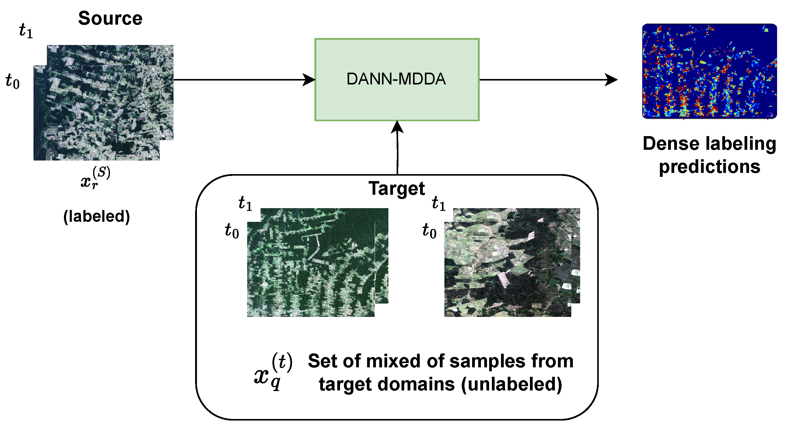
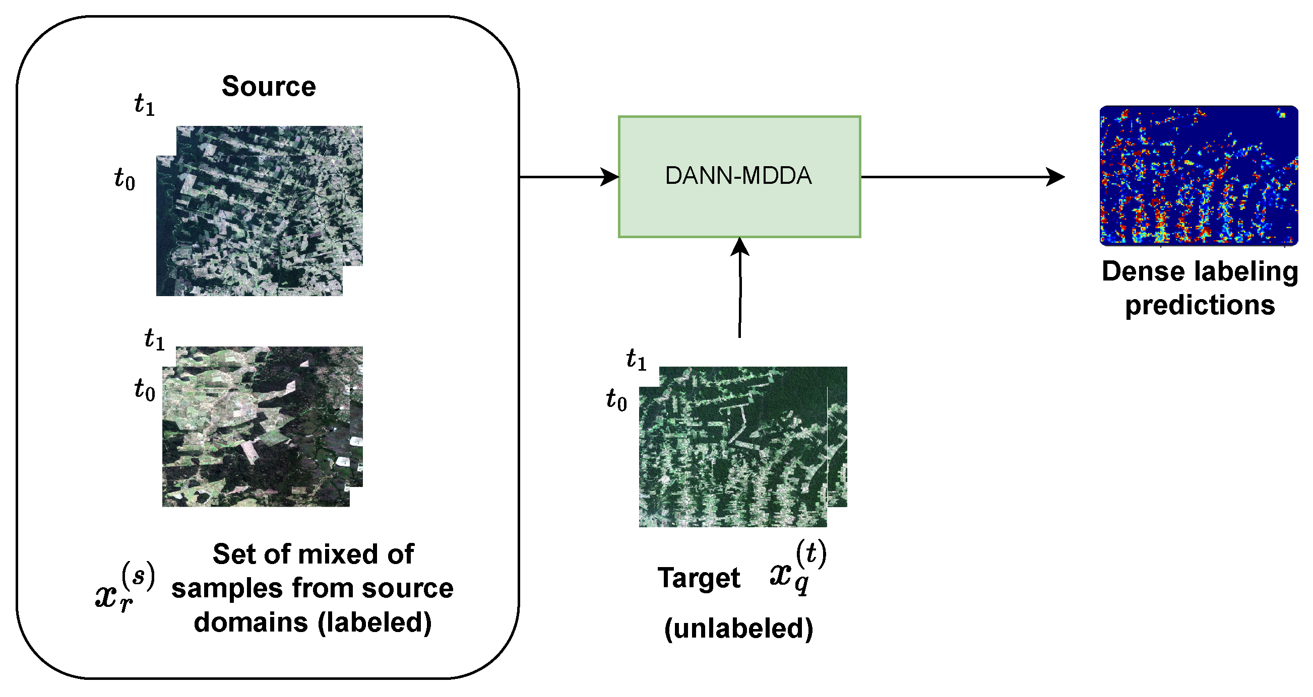
• Two distinct scenarios of domain adaptation (DA) are presented. The first, termed multi-target, involves a single source domain and multiple target domains. The second, known as multisource, consists of multiple source domains adapting to a single target domain;
• Two configurations of the domain discriminator component were evaluated: multi-domain discriminator and source-target discriminator;
• Inclusion and assessment of an expert audit phase designed to target areas of highest uncertainty, utilizing uncertainty estimation from the predictions made by the DL model in a domain adaptation context;
• Experiments are conducted in three different domains associated with Brazilian biomes, and our approach is validated by comparing the results obtained with single-target and baseline experiments.

The remainder of this document is organized as follows. The Section 2 presents materials and methods. Then, in Section 3, we present the experimental procedure, while Section 4 is dedicated to the presentation of the results. Finally, Section 5 is dedicated to a discussion of the results, while Section 6 presents the conclusions.

2. Materials and Methods

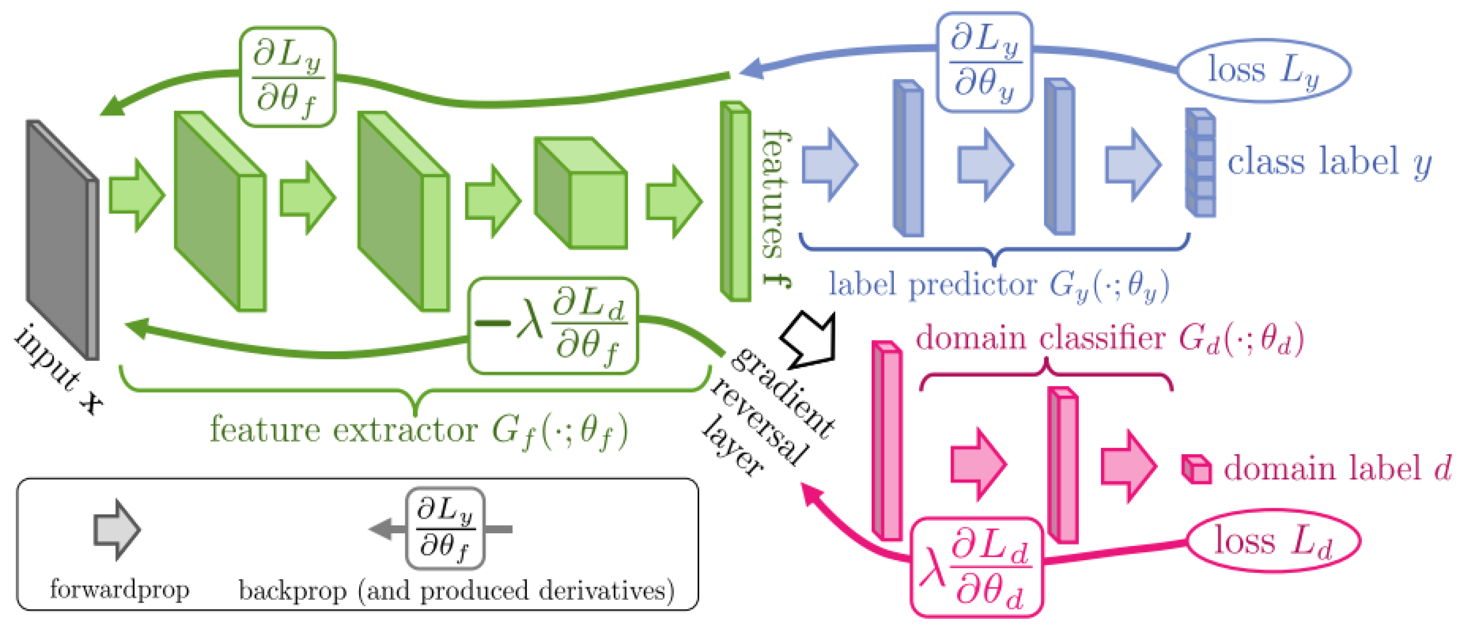
2.1. Domain Adversarial Neural Network (DANN)

Proposed in [29], DANN aims to minimize the divergence between two probability distributions by learning domain-agnostic latent representations by employing adversarial training. As depicted in Figure 1, three modules compose the DANN strategy: a feature extractor $G_f(·,{\theta }_f)$, a label predictor $G_l(·,{\theta }_l)$, and a domain classifier $G_d(·,{\theta }_d)$. In short, $G_f$ maps both the source and target learned features into a common latent space, $G_l$ estimates the input sample categories, and $G_d$, used only during training, tries to discern between source and target samples from the features given by $G_f$.

In the DANN domain adaption strategy, $G_l(·,{\theta }_l)$ does not evaluate features coming from target domain samples, as their corresponding labels are unknown. In contrast, source- and target-domain features are forwarded through $G_d(·,{\theta }_d)$, as their domain labels are known. The optimal network parameters ${\theta }_f^{*},{\theta }_l^{*}$, and ${\theta }_d^{*}$ are given by Equations (1) and (2):

$$({\theta }_f^{*},{\theta }_l^{*})=\arg {\min }_{{\theta }_f,{\theta }_l}E({\theta }_f,{\theta }_l,{\theta }_d^{*})$$

(1)

$$\left({\theta }_d^{*}\right)=\arg {\max }_{{\theta }_d}E({\theta }_f^{*},{\theta }_l^{*},{\theta }_d)$$

(2)

where $E({\theta }_f,{\theta }_l,{\theta }_d)$ represents the DANN loss function defined by

$$E({\theta }_f,{\theta }_l,{\theta }_d)={\mathcal{L}}_l({\theta }_f,{\theta }_l)-\lambda {\mathcal{L}}_d({\theta }_f,{\theta }_d)$$

(3)

The first term in the loss function represents the label predictor loss, and the second term is the domain classifier loss. The $\lambda$ coefficient controls the influence of the domain classifier over the feature extractor parameters. In [29], the authors suggest that $\lambda$ should start and remain equal to zero during the first epochs, allowing the domain classifier to properly learn how to discern among features of the respective domains. Afterwards, the coefficient value gradually increases through the training epochs, favoring the domain classifier influence to the feature extractor in the opposite direction.

As a result, the learning process updates the parameters of the model by implementing the rules detailed in Equations (4)–(6). We observe that $\mu$ and $\lambda$ in the aforementioned equations are both positive. Therefore, the derivatives of ${\mathcal{L}}_d$ push $G_d$ and $G_f$ in opposite directions, configuring an adversarial training, which is expressed by the last term in Equation (6).

This term penalizes $G_f$ when $G_d$ correctly identifies the domain to which an input sample belongs. DANN implements such an operation on Gradient Reversal Layer (GRL) (see Figure 1). Succinctly, during the forward procedure, the GRL acts as an identity mapping and, during the backpropagation, reverses the gradient (multiplying it by $-1$) coming from the domain classifier.

$${\theta }_l={\theta }_l-\mu {\displaystyle \frac{\partial {\mathcal{L}}_l}{\partial {\theta }_l}}$$

(4)

$${\theta }_d={\theta }_d-\mu {\displaystyle \frac{\partial {\mathcal{L}}_d}{\partial {\theta }_d}}$$

(5)

$${\theta }_f={\theta }_f-\mu {\displaystyle \frac{\partial {\mathcal{L}}_l}{\partial {\theta }_f}}+\lambda \mu {\displaystyle \frac{\partial {\mathcal{L}}_d}{\partial {\theta }_f}}$$

(6)

It can be noted in Figure 1 that the outputs of the label predictor are class probabilities, as the DANN strategy was originally proposed for image classification [33]. In the network architecture implemented in this work, the label predictor actually performs semantic segmentation, or dense labeling, individually classifying image pixels. Additionally, as also shown in Figure 1, originally, the output of the domain classifier was binary, as it only had to distinguish between two classes: source or target. We anticipate that, in the proposed method, this is not necessarily the case, as more than two domains are considered. This is detailed in the next section.

2.2. Dense Multi-Domain Adaptation

This work proposes an approach called Domain Adversarial Neural Network Dense Multi-Domain Adaptation (DANN–DMDA) to tackle the challenges of deforestation detection by exploring two settings. In the first, called Multi-Target DA, a set of a labeled source domain is incorporated alongside multiple sets of unlabeled target domains, combined into a single one for adaptation. In the second setting, called Multi-Source DA, we combine multiple labeled source domains into a single one to adapt to a single unlabeled target domain. The hypothesis is that utilizing domain adaptation with multiple unlabeled target domains or multiple labeled source domains can improve the accuracy of deforestation prediction across these domains. Using both diverse target and source domains, the model can learn a more robust and generalized feature representation.

This work builds on the method proposed by [30], which introduced an unsupervised domain adaptation approach for deforestation detection. Additionally, the Deeplabv3+ semantic segmentation architecture was employed, as evaluated in [30] (please refer to Section 2.3).

Like DANN, the DANN–DMDA approach employs two adversarial neural networks: the domain discriminator and the label predictor. The architecture includes an encoder model that transforms input samples into a latent representation, a decoder responsible for semantic segmentation, and a domain discriminator that attempts to classify the domain of the encoder’s output (determining whether it belongs to the source or target domain). In the multi-target configuration, the encoder component receives a set of labeled samples from one source domain and unlabeled samples originating from two or more distinct target domains. Alternatively, in the multi-source setting, the encoder is provided with labeled samples from two or more source domains, and unlabeled samples from a single target domain.

By employing such an architecture and training methodology, we aim to obtain a common feature representation shared across all domains involved and thus improve the performance of semantic segmentation on each target domain. Although our method can be generalized to multiple target domains, we make use of two targets only to showcase the method and experiments.

Figure 2 and Figure 3 illustrate in a simplified way the blend of target and source samples for domain adaptation.

The proposed method follows the general structure outlined by [24,28,30], which consists of three phases: data pre-processing, training, and evaluation.

First, there is a data pre-processing phase, which consists of the following procedures. The first is to apply the Early Fusion (EF) procedure, which concatenates images taken at different periods of time in the spectral dimension. Then, each image is partitioned into tiles, which are then allocated to training, validation, and test sets. From each tile, small patches are extracted to be used as input to the DANN–DMDA model.

The training phase comes in sequence. We define two distinct designs for the domain classifier model. In the first, called the multi-domain discriminator, the discriminator label space is ${\mathcal{Y}}^d=\{0,1,\dots ,d-1\}$, where each class is represented by a unique value. In the other design, named source-target discriminator, the label space is ${\mathcal{Y}}^d=\{0,1\}$, where 0 denotes the source domain and 1 represents the target domain. In this case, there is no discrimination between specific source or target domains. For the label predictor model, a pixel-wise weighted cross-entropy loss is adopted in order to enable a calibration over of how much weight is given to no-deforestation and deforestation predictions. The domain discriminator model works with a cross-entropy loss. The DANN–DMDA model is trained until convergence by simultaneously updating the parameter sets $\{{\theta }_f,{\theta }_y,{\theta }_d\}$.

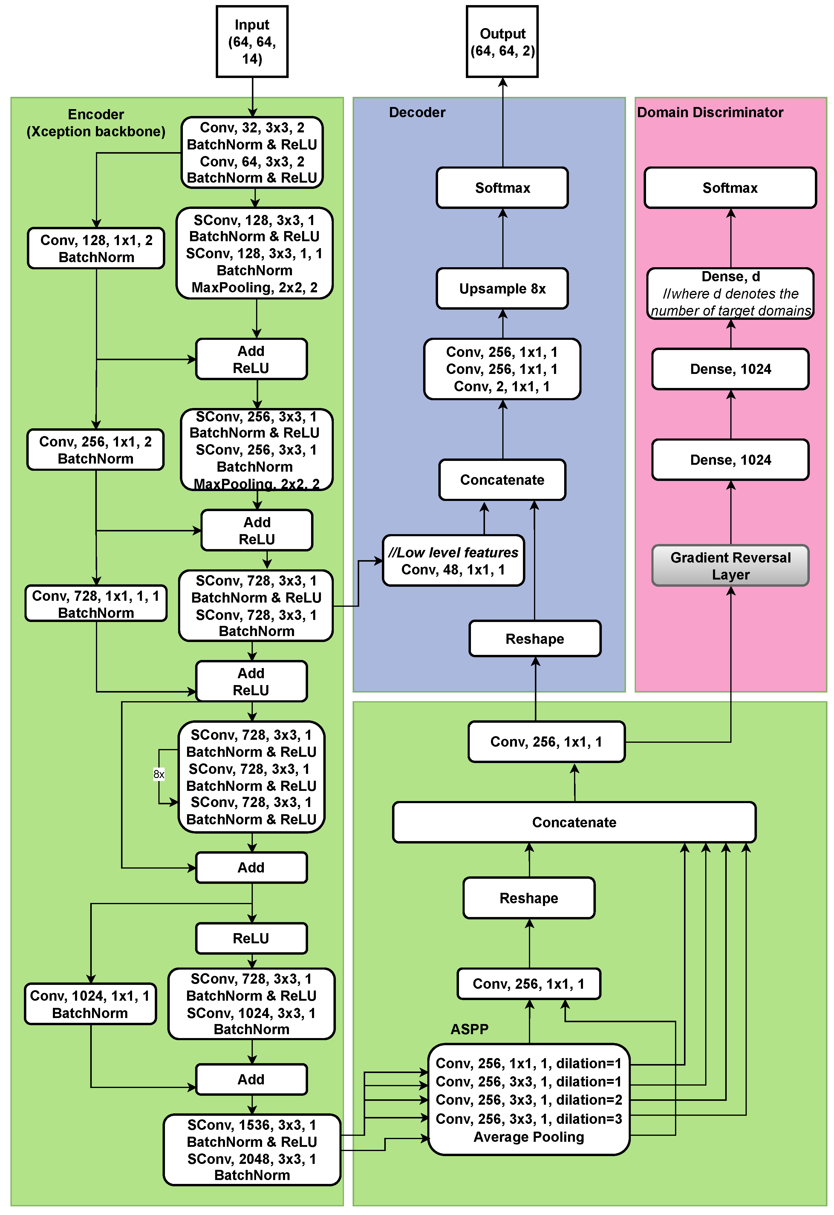
2.3. Deep Learning Model Architecture

The DMDA model developed in this study extends an adapted version of the Deeplabv3+ architecture introduced in [30]. The encoder backbone relies heavily on Xception [34], although some adjustments have been made to adapt the network to the problem and the input data. The dilation rates of the atrous convolutions in the ASPP have been modified to 1, 2 and 3, replacing the original rates of 6, 12, and 18 [31].

Figure 4 provides a visual representation of the deep learning architecture. The layer descriptions include the following information: convolution type (“Conv” for regular strided convolution and “SConv” for depthwise separable convolution), number of filters, filter size, and stride. The ASPP component displays dilation rate values. BatchNorm indicates batch normalization, and ReLU is the activation function.

2.4. Uncertainty Estimation

Uncertainty in machine learning can be broadly categorized into aleatoric and epistemic. Aleatoric uncertainty is associated with intrinsic randomness in the data—it is inherent and irreducible. Epistemic, or model uncertainty, arises from an imperfect fit of the model to the data. Unlike aleatoric uncertainty, epistemic uncertainty can be reduced as more data become available or the model’s complexity is adjusted [35]. Recent advances have provided novel approaches to model and quantify both types of uncertainty.

In the particular case of deforestation detection, Martinez et al. [32] evaluated different uncertainty estimation methods, i.e., evidential deep learning [36], Monte Carlo dropout [35], and deep ensembles [37]. Different uncertainty metrics were also evaluated, i.e., predictive entropy, predictive variance, and mutual information. Martinez et al. [32] concluded that best results in terms of uncertainty estimation for deforestation detection were obtained using deep ensembles and predictive entropy, which is why, in this work, we chose to work with those techniques. We acknowledge that, as the network architectures used in [32] and in our work are different, it would be interesting to evaluate the alternative possibilities, but we will leave that for a future investigation.

The ensemble is composed of a set of instances of the architecture shown in Figure 4. Each instance is trained with different random initializations of network weights and different batch selections, resulting in K different models. The uncertainty of the pixel-wise predictions is assessed by calculating the predictive entropy for the K models, as in Equation (7), in which ${\mu }_k$ is a model’s output probability map. In the following experiments, K was arbitrarily chosen as five, given the computational resources and time that each training session requires. The result is an uncertainty map with the same spatial dimensions as the prediction map. It is important to emphasize that the computational cost of uncertainty estimation is minimal when compared to ensemble prediction and model training. This is because the uncertainty computation reuses the probability maps already generated during the test phase of each training session.

$$H\left(\mu \right)=-{\displaystyle \frac{1}{K}}\sum _{k=1}^K{\mu }_{k}log\left({\mu }_k\right)$$

(7)

To classify predictions as having high or low uncertainty, the uncertainty threshold Z is determined based on the audit area parameter $AA$, defined in terms of the percentage of the total area. The uncertainty map values are sorted and the threshold Z is set at the $100-AA$ percentile. The regions with high uncertainty are then selected for manual inspection. The goal is to find a threshold that optimizes the F1-Score while minimizing manual review effort.

We adopted $F_{1_{low}}$ for samples with uncertainty below the threshold defined by the $AA\%$-most uncertain pixels, which are subjected to audit. Contrarily, $F_{1_{high}}$ considers the pixels with the highest uncertainty values $AA\%$. $F_1$ represents the classification accuracy prior to auditing, and $F_{1_{aud}}$ the classification performance after a human expert visually inspects and correctly annotates the high-uncertainty regions. In this study, we simulate the inspection process by replacing the most uncertain pixels using their respective ground truth labels. It should be noted that this method of review for the uncertainty areas can be applied to a model trained without domain adaptation as well since it is independent of the training approach.

3. Experimental Protocol

3.1. Experiment Plan

This study included four types of experiments:

• Baselines: Validation of the deep learning architecture and establishment of reference benchmarks;
• DMDA multi-target;
• DMDA multi-source;
• Uncertainty estimation with review phase.

The architecture and domain adaptation (DA) methods were validated across various training and testing configurations. Regarding the baseline experiments, the models were evaluated by training and testing on the same domain (Training on target), which serves as the upper-bound baseline, and by training on one source domain and testing on a different target domain (Source-only training), serving as the lower-bound baseline. Additionally, a single-target scenario was assessed to further validate the DA methods.

In order to verify the success of the proposed DANN–DMDA approach, multi-target, multi-source, and uncertainty estimation experiments were conducted over all possible combinations of the three domains. In addition, to ensure the reliability of the results, standard deviation and hypothesis tests were conducted based on the F1-Score from five independent runs of each experiment. The multi-domain experiments were evaluated for superiority over the lower baseline.

In each experiment, in the multi-target scenario, one domain dataset worked as the source domain, providing labels, whereas the other two domains were used as targets. Alternatively, in the multi-source setting, in each experiment, two domains were used as sources, while another domain was used as target. For example, in the Source MA | Target PA combination, the RO domain was incorporated as an additional domain in DMDA experiments.

Regarding the uncertainty estimation for the review phase, to simplify the experiments and maintain comparability with [32], the audit area has been arbitrarily fixed as 3%.

3.2. Datasets

The dataset, previously used in [30], consists of pairs of images from different sites within the Amazon and Cerrado biomes, located in the Brazilian states of Rondônia (RO), Pará (PA), and Maranhão (MA). The selected forest domains represent a range of forest types, from dense forests with small variations in canopy structure, to those with high variability. The class distribution is highly imbalanced in all domains. The images used were captured by the Landsat 8-OLI sensor, which has a 30 × 30 m spatial resolution and seven spectral bands. They were downloaded from the USGS Earth Explorer website. The reference data on deforestation were generated by the PRODES project and are freely available at the Terrabrasilis website (https://terrabrasilis.dpi.inpe.br/app/map/deforestation), accessed on 16 July 2024. The images that comprise the dataset used in this work were exactly the same ones used in PRODES for deforestation assessment in the respective years and locations. Furthermore, all images were captured during July and August for optimal cloud coverage. Similar to [30], the image space of each domain was partitioned into tiles (large subsets of the images).

To ensure a fair comparison between different methods, the same images and experimental protocols used in [24,26] were used in this work. Information regarding image dates, vegetation typology, and class distribution are presented in

Table 1. Information of each domain: image acquisition dates, classes distribution, and vegetation typology.

Domains	RO	PA	MA
Vegetation	Open Ombrophilous	Dense Ombrophilous	Seasonal Deciduous and Semi-Deciduous
Date 1	18 July 2016	2 August 2016	18 August 2017
Date 2	21 July 2017	20 July 2017	21 August 2018
Deforested pixels	225,635 (2%)	82,970 (3%)	71,265 (3%)
Not deforested pixels	3,816,981 (29%)	1,867,929 (65%)	1,389,844 (57%)
Previously deforested pixels	9,013,384 (69%)	903,901 (65%)	986,891 (40%)

. Figure 5 illustrates the studied regions.

3.3. Model Training Setup

The image space within each domain was divided into tiles or large image subsets. Specifically, 100 tiles were defined for the RO image, while the PA and MA images were divided into 15 tiles each. For the RO tiles, approximately 20% were utilized for extracting training patches/samples, which are small image subsets matching the classifier input size; 5% of the tiles were assigned for extracting validation patches; and the remaining 75% were allocated for testing. In the case of the PA and MA images, 26% of the tiles were designated for training; 13% for validation; and 60% for testing.

Table 2. Additional information on each domain dataset.

Domains	RO	PA	MA
Dimension (pixels)	2550 × 5120	1098 × 2600	1700 × 1440
Tiles (image subsets)	100	15	15
Tiles for training	2, 6, 13, 24, 28, 35, 37, 46, 47, 53, 58, 60, 64, 71, 75, 82, 86, 88, 93	1, 7, 9, 13	1, 5, 12, 13
Tiles for validation	8, 11, 26, 49, 78	5, 12	6, 7
% for training	20%	26%	26%
% for validation	5%	13%	13%
% for testing	75%	60%	60%

and Figure 6 give an overview of how the dataset has been organized.

Following previously published studies on the current dataset, e.g., [24,26,28,30,38], certain image areas were masked and excluded during the training and testing phases to ensure proper model evaluation. The masked areas include (i) regions affected by deforestation prior to the date of the first image in the pair; (ii) a two-pixel buffer surrounding deforestation polygons; and (iii) deforestation polygons smaller than 6.25 hectares (69 pixels) in Amazon sites and polygons smaller than 1 hectare (11 pixels) in the Cerrado site. The first restriction was applied because the reference data does not provide information on previously deforested areas; once PRODES detects deforestation, the affected regions remain classified as deforested regardless of subsequent changes. The second condition helps to mitigate the impact of minor inaccuracies in deforestation references caused by the rasterization process. As for the third constraint, we adhered to PRODES criteria, as deforestation polygons smaller than the specified thresholds are not mapped by it.

Following data pre-processing, the domain patches are employed to train the proposed domain adaptation (DA) methods, whose settings and hyper-parameters are described next.

The extracted samples from image pairs across all domains consist of patches measuring 64 × 64 pixels, with 14 channels. Data augmentation techniques, including 90-degree rotation, as well as vertical and horizontal flips, were applied to the patches in both the source and target domains. In line with [30], we utilized the Adam optimizer and incorporated learning rate decay during the training process, whose formula is described in Equation (8):

$${\mu }_p={\displaystyle \frac{{\mu }_0}{{\left(1+\alpha ·p\right)}^{\beta }}}$$

(8)

Following Ganin et al. [33], the initial learning rate ${\mu }_0$ was set to $1\times {10}^{-4}$, while $\alpha$ was assigned as 10 and $\beta$ was set to 0.75. Here, p represents the training progress, which changes from 0 to 1, following the advance of the epochs.

The gradient reversal layer parameter $\lambda$ is initially set to 0 and progressively updated over the epochs following the function defined in Equation (9), which was also proposed by Ganin et al. [33]. This scheduling strategy aims to gradually amplify the strength of gradient reversal during backpropagation from the domain discriminator, encouraging the feature extractor to learn more domain-invariant representations over time. Among the alternatives, empirically evaluated during the development of this work, we adopted the formulation proposed by [33] (Equation (9)), as it yielded the best results. The parameter $\gamma$ was set to 2.5, following [30].

$$\lambda ={\displaystyle \frac{2}{(1+exp(-\gamma ·p\left)\right)}}$$

(9)

A batch size of 32 was employed, and an early stopping procedure was implemented to prevent overfitting. Moreover, following [28], for the loss functions, we set ${\mathcal{L}}_y$ and ${\mathcal{L}}_d$ to be a weighted cross-entropy function and a categorical cross-entropy, respectively. During the training procedure, the model that was considered the best achieved both the lowest value for ${\mathcal{L}}_y$ and the highest value for ${\mathcal{L}}_d$. This indicated strong performance on the primary task of deforestation prediction, while also ensuring that the encoder effectively fooled the discriminator, making it unable to distinguish the domain of the sample. Following Torres et al. [39], the weights have been set to 2 and 0.4 for the deforestation and no-deforestation class, respectively. This approach has been employed to address the issue of the highly imbalanced distribution between deforestation and no-deforestation pixels.

3.4. Hardware and Configuration

The DANN model and Deeplabv3+ were implemented in Python 3.6 on top of Tensorflow 1.15 (https://www.tensorflow.org/), accessed on 1 October 2024, which is an open-source library widely used for machine learning and deep learning tasks. The experiments were run on an 64-bit computer, with Ubuntu Linux version 22.04.4 LTS, Intel processor i9-12900F, 12th generation, 128 Gibibytes (GiB) of RAM and NVIDIA GeForce RTX 3090 with 24 GiB of graphics memory. The source code is hosted on Github: https://github.com/LPG-Uerj/FC-DANN_DA_For_CD_MultiTarget_TF2.

3.5. Metrics

The models were evaluated through the semantic segmentation of the input images. In this approach, each pixel within the input image provided to the network was assigned to one of two classes: deforestation or no-deforestation. Due to the significant class imbalance in the dataset, where deforested areas represent only a small fraction of the total, global accuracy is not among the most appropriate metrics for evaluating that models. To evaluate the performance of the classifiers in each scenario, the average F1-Score (Equation (10)), precision (Equation (11)), and recall (Equation (12)) were calculated.

These metrics focused on the positive (deforestation) class. The F1-Score is determined by computing the harmonic mean of the precision and recall values, as shown below in Equation (10):

$$F_1-Score={\displaystyle \frac{2\times Precision\times Recall}{Precision+Recall}}$$

(10)

where

$$Precision={\displaystyle \frac{TP}{TP+FP}}$$

(11)

$$Recall={\displaystyle \frac{TP}{TP+FN}}$$

(12)

In Equations (11) and (12), the number of true positives ($TP$) represents the pixels correctly assigned to the deforestation class, while the number of false positives ($FP$) corresponds to the pixels mistakenly classified as deforestation. The false negatives ($FN$) indicate the number of pixels that were incorrectly classified as no-deforestation.

To ensure comparability with previous studies, recall, precision and F1-Score metrics were calculated using a standard threshold of 0.5 for predictions. Probabilities below 0.5 were classified as no-deforestation, while those above were classified as deforestation.

4. Results

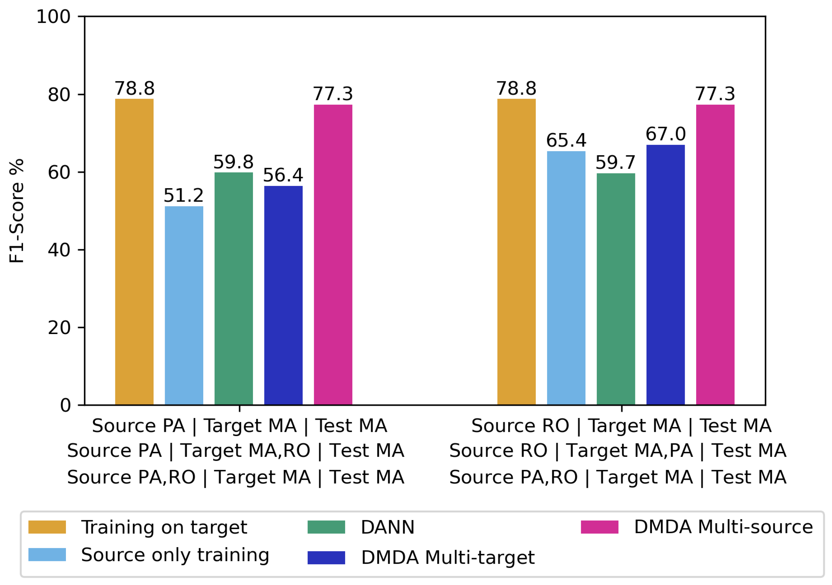
4.1. Baseline and Multi-Target Results

Table 3. Evaluation of F1-Score and standard deviation in multi-target experiments. Bold values represent the highest scores, while italicized values indicate the second-highest.

Source	MA				PA				RO
Target *	PA,RO		PA,RO		MA,RO		MA,RO		MA,PA		MA,PA
Test	PA		RO		MA		RO		MA		PA
Experiments	F1	$\mathit{\sigma }$	F1	$\mathit{\sigma }$	F1	$\mathit{\sigma }$	F1	$\mathit{\sigma }$	F1	$\mathit{\sigma }$	F1	$\mathit{\sigma }$
Training on target	81.0	$\pm 0.37$	68.0	$\pm 1.24$	78.8	$\pm 5.90$	68.0	$\pm 1.24$	78.8	$\pm 5.90$	81.0	$\pm 0.37$
Source-only training	70.3	$\pm 4.00$	47.3	$\pm 6.72$	51.2	$\pm 3.62$	20.9	$\pm 3.00$	65.4	$\pm 2.10$	40.8	$\pm 2.34$
Single-target DA	68.8	$\pm 2.58$	59.1	$\pm 3.64$	59.8	$\pm 4.33$	31.8	$\pm 3.77$	59.7	$\pm 4.37$	57.1	$\pm 2.54$
DMDA Multi-target multi-domain disc.	69.3	$\pm 2.66$	58.5	$\pm 5.05$	56.4	$\pm 3.87$	36.3	$\pm 1.86$	67.0	$\pm 7.71$	57.7	$\pm 2.13$
DMDA multi-target source-target disc.	70.8	$\pm 1.69$	55.4	$\pm 2.59$	55.5	$\pm 3.70$	31.5	$\pm 5.34$	67.8	$\pm 4.97$	57.3	$\pm 4.18$

* Used in multi-target experiments. In single-target DA, the training and test domains are the same.

presents the baseline along with multi-target results, highlighting the best outcomes for each source–target combination. It is interesting to observe the drop in performance in the baseline results. The line Training on target shows the accuracies obtained when training and testing the DL model on the target domain, without domain adaptation. The respective accuracy values can be regarded as the upper-bound baseline. The line Source-only training shows the accuracies obtained when training the model with source-domain samples and testing with target samples, without DA. The respective accuracy values can be regarded as the lower-bound baseline. The differences between the lower- and upper-bound baselines are manifestations of the domain shift between the respective domains. The larger the difference, the higher the domain shift. However, for each domain combination, the roles of the domains, i.e., source or target, also matter in the accuracy drops, that is, the differences between the baselines are not symmetrical. Although this happens in any domain adaptation problem, explaining this lack of symmetry is an open question in domain adaptation research, but we believe it has to do with the differences in the complexity of the domains, as is discussed in Section 5.

It can be seen in Table 3 that DMDA Multi-Target generally outperformed both Single-target DA and Source-only training. The Multi-target multi-domain discriminator achieved the highest F1-Score in Source PA | Target MA,RO | Test RO and Source RO | Target MA,PA |Test PA combinations, while the Multi-target source-target Discriminator performed best in Source RO | Target MA,PA | Test MA and Source MA | Target PA,RO | Test PA. Both DMDA setups reversed the negative transfer observed in Single-target DA for Source RO | Target MA. However, Single-target DA was optimal for Source MA | Target RO, indicating that adding PA did not enhance accuracy. These results suggest that multi-target training can reduce domain shift in an unsupervised target scenario. The multi-domain discriminator generally outperforms the source-target discriminator, except in the Source RO | Target MA,PA | Test MA and Source MA | Target PA,RO | Test PA cases, which deserves further investigation.

Table 4. Hypothesis tests based on Welch’s t-test. Acc. denotes the accepted hypothesis while p-val represents the p-value calculated for the pair of experiments compared.

Source	MA				PA				RO
Target *	PA,RO		PA,RO		MA,RO		MA,RO		MA,PA		MA,PA
Test	PA		RO		MA		RO		MA		PA
Pairs of Experiments	Acc.	p-Val	Acc.	p-Val	Acc.	p-Val	Acc.	p-Val	Acc.	p-Val	Acc.	p-Val
DMDA Multi-target Multi-Domain Disc. vs. Source-only training	H0	0.26	H1	0.01	H0	0.06	H1	<0.01	H0	0.55	H1	<0.01
DMDA Multi-target Source-Target Disc. vs. Source-only training	H0	0.15	H1	0.02	H0	0.20	H1	<0.01	H0	0.77	H1	<0.01

* Used in multi-target experiments. In single-target DA, the training and test domains are the same.

presents the statistical significance tests used to assess whether multi-target models outperform Source-only training baseline values. The analysis is based on the F1-Score results from five independent runs of each experiment. The null hypothesis (H0) assumes that both approaches yield equal mean F1-Scores, while the alternative hypothesis (H1) claims that multi-target models achieve superior performance. Given the unequal variances observed between the compared samples, Welch’s t-test is employed as the appropriate statistical method. A p-value threshold of 0.05 is adopted to determine statistical significance. The experiments Source MA | Target PA,RO | Test RO; Source PA | Target MA,RO | Test RO; and Source RO | Target MA,PA | Test PA are statistically superior compared to the Source-only training baselines.

4.2. Multi-Source Results

In the multi-source setting, two domains were combined as sources (i.e., containing class labels), while a third served as the target domain. Three multi-source experiments were conducted: (i) Multi-source only training, where no domain adaptation was employed; (ii) DMDA Multi-source multi-domain discriminator; and (iii) DMDA Multi-source source-target discriminator, both of which incorporated domain adaptation.

Table 5. Evaluation of F1-Score and standard deviation in multi-source experiments. Values in bold represent the highest, while values in italic indicate the second highest. Superscripts ¹ and ² indicate the distinct source domains used separately in the Source-only training experiments. Specifically, Source-only training ¹ refers to the experiment conducted using domain ¹ as the sole source domain, while Source-only training ² corresponds to the experiment using domain ² as the source.

Source	MA 1, PA 2		PA 1, RO 2		MA 1, RO 2
Target	RO		MA		PA
Test	RO		MA		PA
Experiments	F1	$\mathit{\sigma }$	F1	$\mathit{\sigma }$	F1	$\mathit{\sigma }$
Source-only training 1	47.3	$\pm 6.72$	51.2	$\pm 3.62$	70.3	$\pm 4.00$
Source-only training 2	20.9	$\pm 3.00$	65.4	$\pm 2.10$	40.8	$\pm 2.34$
Multi-source only training (No DA)	44.2	$\pm 2.33$	77.8	$\pm 1.89$	62.4	$\pm 2.71$
DMDA Multi-source multi-domain Disc.	52.8	$\pm 3.79$	77.3	$\pm 3.61$	67.6	$\pm 2.56$
DMDA Multi-source source-target Disc.	53.4	$\pm 3.44$	77.5	$\pm 3.70$	67.1	$\pm 7.48$

highlights key findings. First, DMDA methods consistently improved performance over multi-source-only training in two out of three experiments, demonstrating its benefits even when using multiple source domains. Second, unlike in the multi-target experiments, neither configuration of the discriminator component in DMDA multi-source yields a meaningful improvement in F1-Score.

Table 6. Hypothesis tests based on Welch’s t-test. Acc. denotes the accepted hypothesis while p-val represents the p-value calculated for the pair of experiments compared. Given that both multi-source configurations present similar results, only DMDA Multi-source multi-domain Disc. was tested against Source-only training baselines. Superscripts ¹ and ² indicate the distinct source domains used separately in the Source-only training experiments. Specifically, Source-only training ¹ refers to the experiment conducted using domain ¹ as the sole source domain, while Source-only training ² corresponds to the experiment using domain ² as the source.

Source	MA 1, PA 2		PA 1, RO 2		MA 1, RO 2
Target	RO		MA		PA
Test	RO		MA		PA
Experiments	Acc.	p-Val	Acc.	p-Val	Acc.	p-Val
Multi-source only training (No DA) vs Source-only training 1	H0	0.67	H1	<0.01	H0	0.98
Multi-source only training (No DA) vs. Source-only training 2	H1	<0.01	H1	<0.01	H1	<0.01
DMDA Multi-source multi-domain Disc. vs. Source-only training 1	H1	0.04	H1	<0.01	H0	0.88
DMDA Multi-source multi-domain Disc. vs. Source-only training 2	H1	<0.01	H1	<0.01	H1	<0.01

presents the statistical significance tests used to assess whether multi-source models outperform source-only training baselines. The null hypothesis (H0) and alternative hypothesis (H1) follow the protocol employed in multi-target tests.

4.3. Overall Multi-Domain Results

This section compares model performance across single-target DA, DMDA multi-target, and DMDA multi-source. The Multi-Domain Discriminator was used in the latter two, given its superior performance in most experiments. Results are analyzed against both lower- and upper-bound baselines.

Figure 7 illustrates results for target MA, where combining PA and RO as sources significantly improved F1-Score, nearing the upper bound of 78.8%. As for target PA (Figure 8), adding RO to Source MA | Target PA | Test PA did not yield improvements, suggesting limited transferability between PA and RO. However, incorporating MA into Source RO | Target PA | Test PA significantly enhanced adaptation on multi-domain scenarios. This pattern also appears in Figure 9, where including PA in Source MA | Target RO | Test RO degraded performance, while adding MA to Source PA | Target RO | Test RO multi-domain experiments led to substantial gains in F1-Score.

Overall, these findings reinforce the value of multi-target and multi-source DA, with the multi-domain discriminator proving particularly effective in most configurations.

Table 7. Comparative analysis of methods in terms of F1-Score. In the Domain Pairs column, ‘Source’ denotes the primary labeled domain used for training, while ‘Target’ represents the domain evaluated during testing. The third column, ‘Domain included in multi-domain methods’, specifies the additional domain which was incorporated in multi-target and multi-source experiments.

Domain Pairs (Source-Target)	Single-Target DA Compared to Lower-Bound	Domain Included in Multi-Domain Methods	DMDA Multi-Target Multi-Domain Disc. Compared to Single-Target DA	DMDA Multi-Source Multi-Domain Disc. Compared to Single-Target DA
PA-RO	+10.9	MA	+4.5	+21.0
RO-PA	+16.3	MA	+0.6	+10.5
PA-MA	+8.6	RO	−3.4	+17.5
MA-RO	+11.8	PA	−0.6	−6.3
RO-MA	−5.7	PA	+7.3	+17.6
MA-PA	−1.5	RO	+0.5	−1.2

synthesizes the contribution in terms of F1-Score gain in a third domain in multi-domain methods. The second column, single-target DA compared to lower-bound, shows the contribution of the target in the adaptation training compared to source-only training. Including the MA domain in the multi-domain training improved the model’s performance when tested on both the RO and PA domains. This improvement may be attributed to the high complexity of forested areas in that region, driven by greater environmental variability. The presence of prolonged dry periods throughout the year leads to natural vegetation loss not associated with deforestation.

Another key finding is that introducing PA as a third domain benefits the model when tested on MA (RO-MA) but degrades performance compared to the single-target DA setting for MA-RO. A similar trend is observed with RO as the third domain: it enhances results in the multi-source experiment for PA-MA but remains comparable to single-target DA for MA-PA, showing minor gains and losses in multi-target and multi-source scenarios, respectively. This behavior may stem from the fact that PA and RO share a more homogeneous and dense forest structure, along with a higher proportion of progressive degradation, a more challenging feature to detect compared to the MA domain.

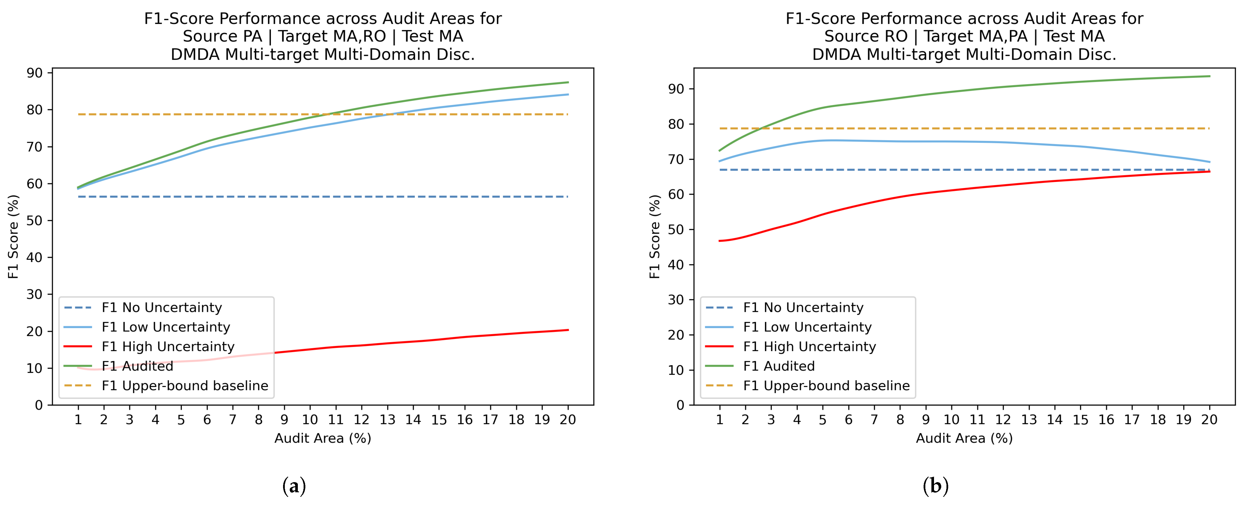
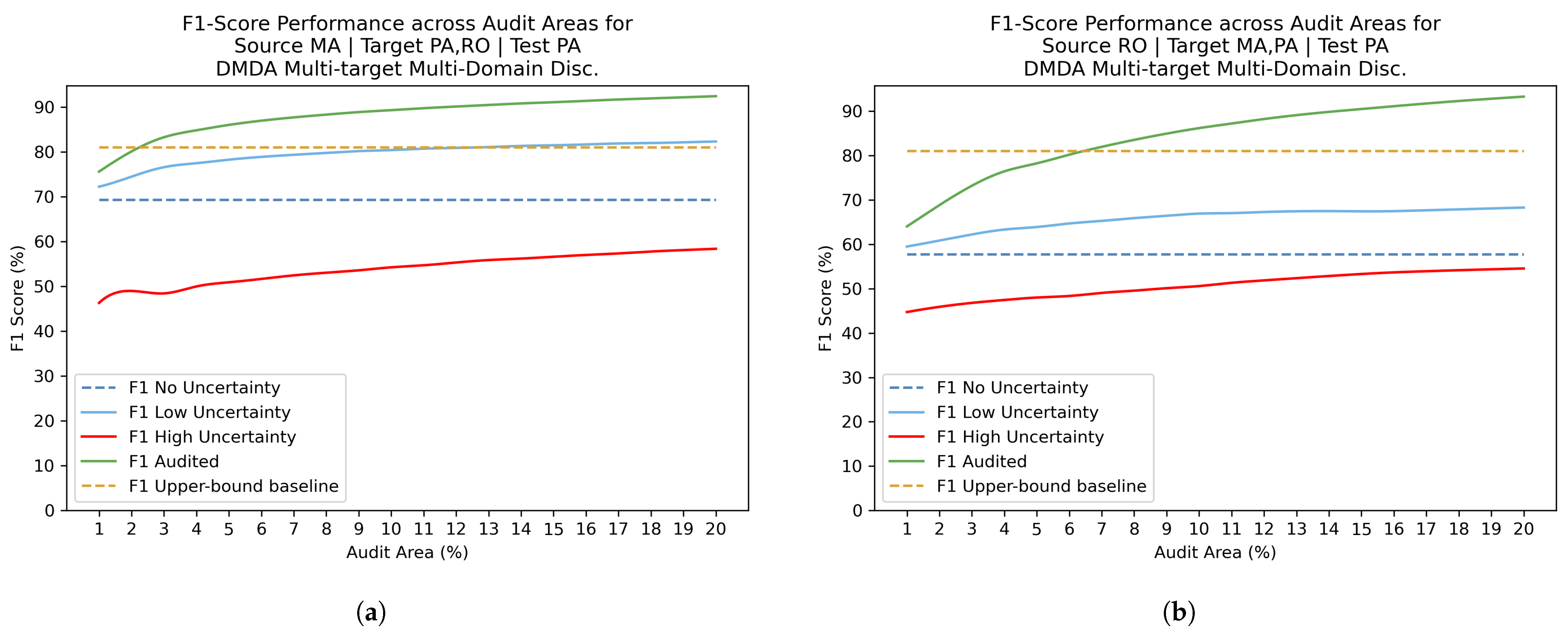
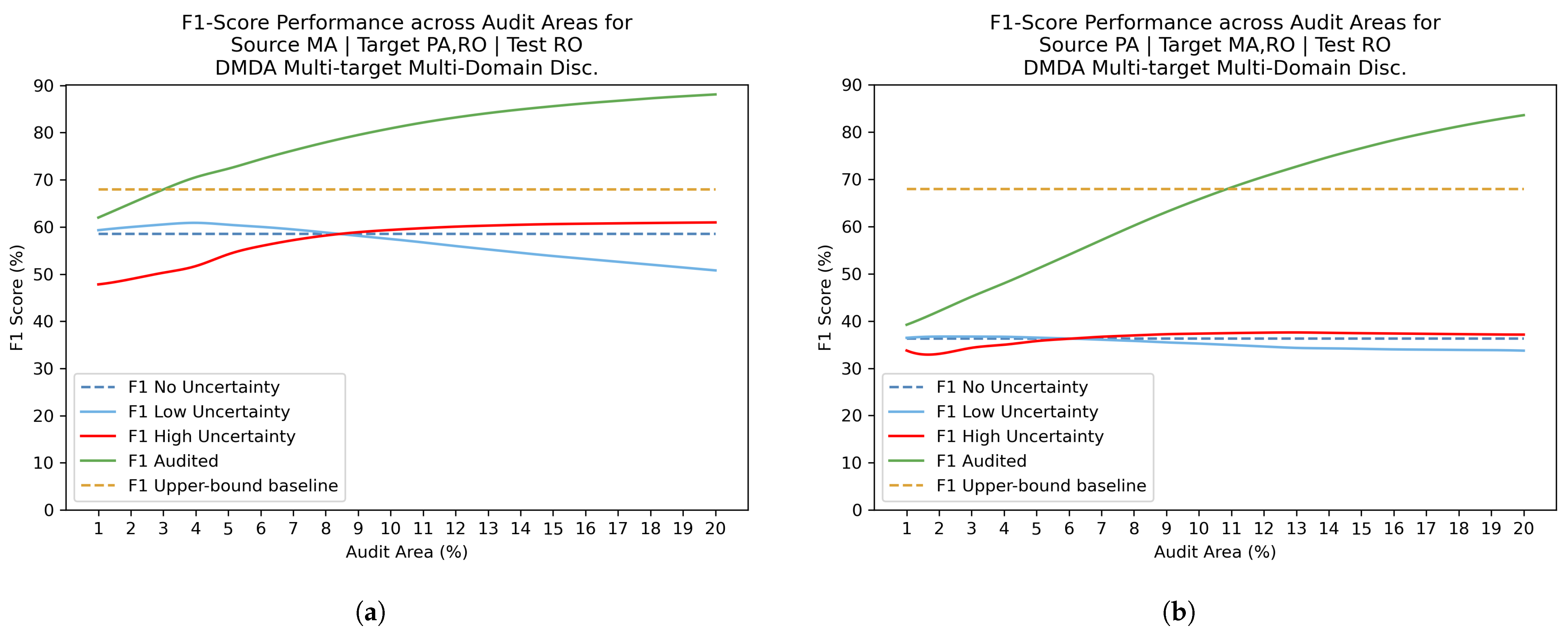
4.4. Uncertainty Estimation with Review Phase Results

After domain adaptation training procedures, an uncertainty estimation with review phase was included to the study. F1-Scores were calculated for discrete audit area values ranging from 1% to 20%. Figure 10, Figure 11 and Figure 12 present the F1-Score values in different scenarios: without uncertainty filtering, calculated only over low-uncertainty pixels, calculated over high-uncertainty pixels, and after applying the audit process. The observed pattern revealed that the F1-Score for high-uncertainty predictions consistently exhibited the lowest values, while the F1-Score for low-uncertainty predictions surpassed the original F1-Score obtained without audit. This finding supports the hypothesis that strong F1 performance is associated with predictions characterized by low uncertainty. Nonetheless, Figure 12 reveals an intriguing observation: for the configurations Source MA | Target PA and Source RO | Target PA, the low-uncertainty and high-uncertainty lines intersect when the audit areas exceed 8% and 6%, respectively. This indicates that, for the RO target, larger audit areas diminish the effectiveness of the threshold in distinguishing between high and low uncertainties. This phenomenon may be attributed to the relative lack of regions predicted with high confidence in the RO domain compared to other target domains. Moreover, our findings reveal that surpassing the upper-bound baseline across all three domains is achievable by auditing at most 11% of the area, as can be seen in Figure 10 and Figure 12.

In most combinations, the F1-audited curve shows its steepest increase between 1% and 5%, after which the this curve reaches its stability regime. The 0–1% range offers the highest F1-Score gain per effort.

To maintain conciseness in the results presentation, uncertainty estimation was applied exclusively to the multi-target experiments. The quantitative results for the uncertainty review are summarized in

Table 8. F1-Score evaluation for MA source in multi-target uncertainty estimation experiments (AA = 3%). Values in bold represent the highest, while values in italic indicate the second highest. ‘Training on target’ values are not highlighted, as they inherently represent the upper bound.

Source	MA
Target *	PA, RO				PA, RO
Test	PA				RO
Experiments	$\mathit{F}\mathbf{1}$	$\mathit{F}{\mathbf{1}}_{\mathit{low}}$	$\mathit{F}{\mathbf{1}}_{\mathit{high}}$	$\mathit{F}{\mathbf{1}}_{\mathit{aud}}$	$\mathit{F}\mathbf{1}$	$\mathit{F}{\mathbf{1}}_{\mathit{low}}$	$\mathit{F}{\mathbf{1}}_{\mathit{high}}$	$\mathit{F}{\mathbf{1}}_{\mathit{aud}}$
Training on target	81.0	89.3	64.3	92.9	68.0	71.7	52.5	77.0
Source only training	70.3	78.0	48.6	84.3	47.3	47.8	45.7	57.9
DA Single-target	68.8	73.1	58.0	81.4	59.1	61.3	50.0	68.8
DMDA Multi-target Multi-Domain Disc.	69.3	76.6	48.4	83.3	58.5	60.5	50.3	67.9
DMDA Multi-target Source-Target Disc.	70.8	77.0	53.6	83.6	55.4	57.4	47.1	65.3

* Used in multi-target experiments. In single-target DA, the target and test domains are the same.

,

Table 9. F1-Score evaluation for PA source in multi-target uncertainty estimation experiments (AA = 3%). Values in bold represent the highest, while values in italic indicate the second highest. ‘Training on target’ values are not highlighted, as they inherently represent the upper bound.

Source	PA
Target *	MA, RO				MA, RO
Test	MA				RO
Experiments	$\mathit{F}\mathbf{1}$	$\mathit{F}{\mathbf{1}}_{\mathit{l}\mathit{o}\mathit{w}}$	$\mathit{F}{\mathbf{1}}_{\mathit{h}\mathit{i}\mathit{g}\mathit{h}}$	$\mathit{F}{\mathbf{1}}_{\mathit{a}\mathit{u}\mathit{d}}$	$\mathit{F}\mathbf{1}$	$\mathit{F}{\mathbf{1}}_{\mathit{l}\mathit{o}\mathit{w}}$	$\mathit{F}{\mathbf{1}}_{\mathit{h}\mathit{i}\mathit{g}\mathit{h}}$	$\mathit{F}{\mathbf{1}}_{\mathit{a}\mathit{u}\mathit{d}}$
Training on target	78.8	86.6	27.5	87.6	68.0	71.7	52.5	77.0
Source-only training	51.2	56.7	9.0	57.7	20.9	19.1	28.9	30.0
DA Single-target	59.8	66.1	10.8	67.1	31.8	30.7	36.8	41.6
DMDA Multi-target multi-domain disc.	56.4	63.1	10.7	64.1	36.3	36.7	34.3	45.2
DMDA Multi-target source-target disc.	55.5	61.3	11.1	62.3	31.5	30.7	34.9	41.6

* Used in multi-target experiments. In single-target DA, the training and test domains are the same.

and

Table 10. F1-Score evaluation for RO source in multi-target uncertainty estimation experiments (AA = 3%). Values in bold represent the highest, while values in italic indicate the second highest. ‘Training on target’ values are not highlighted, as they inherently represent the upper bound.

Source	RO
Target *	MA, PA				MA, PA
Test	MA				PA
Experiments	$\mathit{F}\mathbf{1}$	$\mathit{F}{\mathbf{1}}_{\mathit{low}}$	$\mathit{F}{\mathbf{1}}_{\mathit{high}}$	$\mathit{F}{\mathbf{1}}_{\mathit{aud}}$	$\mathit{F}\mathbf{1}$	$\mathit{F}{\mathbf{1}}_{\mathit{low}}$	$\mathit{F}{\mathbf{1}}_{\mathit{high}}$	$\mathit{F}{\mathbf{1}}_{\mathit{aud}}$
Training on target	78.8	86.6	27.5	87.6	81.0	89.3	64.3	92.9
Source only training	65.4	71.7	41.9	77.0	40.8	37.6	48.9	58.1
DA Single-target	59.7	63.5	47.5	71.3	57.1	60.1	49.9	71.8
DMDA Multi-target Multi-Domain Disc.	67.0	73.2	50.0	79.9	57.7	62.2	46.8	73.2
DMDA Multi-target Source-Target Disc.	67.8	74.9	33.3	77.7	57.3	60.4	48.6	70.6

* Used in multi-target experiments. In single-target DA, the training and test domains are the same.

. Consistent with the methodology used in previous experiments, the Training on target experiment serves as the upper-bound baseline, where the model is trained and evaluated on the same domain. In contrast, the Source-Only Training experiment represents the lower-bound baseline, where the model is trained on one domain and tested on a different domain without utilizing domain adaptation techniques. As expected, in most experiments, the observed pattern was $F_{1_{aud}}\ge F_{1_{low}}\ge F_1\ge F_{1_{high}}$. Human inspections consistently improved model performance, as shown by the $F{1}_{aud}$ metric across all experiments, with results post-inspection correlating with pre-inspection outcomes. That is, when one of the the multi-target experiments outperforms the Source-Only Training for example, this trend continues after auditing. In MA-PA combination, Table 8, post-audit results outperform the original F1 of the model trained on target (upper-bound baseline). In MA-RO source–target pair, DA single-target was also able to surpass the F1-Score from the upper-bound baseline. This outstanding result can also be seen on DMDA Multi-target multi-domain disc. experiment for the RO-MA pair, in Table 10. In contrast, experiments based on PA source, Table 9, did not exceed the original F1-Score from upper-bound baseline, but produced improvements between six and ten points in terms of F1-Score.

5. Discussion

The results indicate that, even with only one labeled source domain, prediction accuracy on a target domain can improve by incorporating an additional unlabeled target domain in the adaptation process. This inclusion helps the model to learn features that are discriminative for the main task while remaining invariant to domain shifts. In the more favorable scenario of multi-source training, with two or more labeled source domains, the model significantly outperforms the lower-bound baseline and leverages the unlabeled data effectively, outperforming the ’Multi-source only training’ experiment. This suggests that both multi-target and multi-source approaches are reliable methods to enhance model performance for deforestation detection. However, substantial gains with multi-source and multi-target domains heavily depend on the diversity of data attributes introduced by additional domains. Regarding the relationship among the three domains used in this study, the inclusion of Maranhão (MA) domain generally improves adaptation for the other domains. This may be explained by the higher complexity and variability of forested areas there. As MA has more dry periods, the visual characteristics of the forest changes without necessarily indicating deforestation. In addition, a model targeting MA is generally benefited from the inclusion of PA or RO as the third domain. Our hypothesis is that, in areas with lower forest density, such as MA, the process of cleaning the area is easier and faster, resulting in more uniform deforestation footprints.

In contrast to other scenarios, the PA site presents a unique challenge due to its higher forest density. This density often results in incomplete deforestation processes, leaving behind debris that may persist for several years. As a consequence, these areas become visually harder to identify as deforested, complicating detection efforts. Both the PA and RO domains exhibit greater diversity in deforested areas, primarily due to the prevalence of clear-cutting with residual vegetation and regions undergoing progressive degradation. This diversity makes it more challenging to accurately classify these areas. When classifiers are trained on one domain (e.g., PA or RO) and applied to the other, they tend to produce a higher rate of false-positive predictions. In simpler terms, the PA and RO domains do not complement each other in terms of predictive accuracy, as the characteristics of deforestation in one domain do not translate well to the other.

A possible explanation for the observed behavior was proposed in [24], which analyzed the complexity of the deforestation and no-deforestation classes in each domain to better understand the performance of a DL-based classifier. In summary, Soto Vega et al. [24] used the number of clusters present in the difference image, computed from the images in the corresponding pairs, to assess the complexity of the deforestation and no-deforestation (forest) classes across domains. The number of clusters was determined using the k-means algorithm in combination with the Calinski–Harabasz [40] criterion to identify the natural number of clusters in each class. The authors hypothesized that the number of clusters correlates with varying forest characteristics and types of changes, thereby reflecting the complexity of the landscape associated with both deforestation and no-deforestation areas.

Accordingly, their results indicated that the complexity of forested regions was lowest in PA and highest in MA. Conversely, the deforested regions in PA exhibited higher complexity, while those in MA showed the lowest. In all cases, the estimated number of clusters aligned with the complexity of the forest canopies characteristic of each site’s forest typology, as well as with the diversity of deforestation practices. In RO, the complexity of both forested and deforested areas fell between the levels observed in PA and MA. Based on these findings, we infer that classifiers trained on MA perform better at identifying changes that are not directly associated with deforestation, while classifiers trained on PA and RO tend to generalize worse due the lower complexity of changes present in their forested areas.

Additionally, by using uncertainty estimation to refine predictions, the F1-Score improved by 6 to 12 percentage points—a notable gain that, in some experiments, even exceeded the upper-bound baseline’s F1-Score. The consistently low F1-Scores in most $F{1}_{high}$ metrics reveal a strong correlation between high uncertainty and prediction error.

We conclude the discussion with an analysis of recent advances in the deforestation detection task. In domain adaptation for remote sensing [41,42,43,44], several authors have explored contrastive learning, self-supervised methods, and Vision Transformer-based architectures [26,45,46,47]. For instance, Kim et al. [46] proposed a contrastive representation learning framework to enhance deforestation detection in noisy satellite images, while Vega et al. [30] leveraged unsupervised pseudo-labeling to mitigate domain shift.

Notably, in a previous work proposed by Vega et al. [38], we evaluated Vision Transformers (ViTs) for deforestation detection on the same dataset. While ViTs demonstrated strong performance when trained and tested within the same domain, their effectiveness in a cross-domain setting was significantly reduced. This suggests that, although Transformer-based models have potential in deforestation detection, their applicability to domain adaptation remains an open question requiring further investigation.

Among adversarial methods, Noa et al. [26] applied Adversarial Discriminative Domain Adaptation (ADDA) with margin-based regularization for deforestation detection on the same dataset. While their approach focuses on single-source to single-target adaptation, our method builds upon adversarial adaptation by incorporating a multi-source, multi-target paradigm. This extension enables improved generalization across multiple domains, addressing dataset variability more effectively. Our results, although comparisons are not straightforward, indicate that this approach leads to higher accuracy, mostly in RO and PA, demonstrating the advantages of multi-source domain adaptation in deforestation monitoring.

6. Conclusions

The proposed approach learns invariant feature representations across multiple domains, whether source or target. This is achieved by strategically selecting samples from different domains and modifying the domain discriminator to predict the specific domain of each sample. Experimental results demonstrate that DMDA multi-target outperformed single-target DA in four out of six cross-domain experiments. Furthermore, DMDA multi-source surpassed both DMDA multi-target and single-target DA in four out of six domain pair combinations, highlighting its effectiveness in improving prediction accuracy without requiring additional labeled data. While the success of multi-domain scenarios depends on the characteristics of the domains incorporated during training, these methods, given the increased diversity of training data—whether as source or target—tend to produce more balanced models in terms of accuracy. Although they may not always achieve the highest accuracy, they help to mitigate negative transfer.

Additionally, targeted human review can further boost model accuracy with a relatively modest effort. In the context of remote sensing for deforestation detection, combining unsupervised multi-domain adaptation with uncertainty estimation to guide human intervention proves to be an effective strategy for significantly improving model classification performance. However, it must be highlighted that human review is a technique that can be applied independently of the model, with or without adaptation, allowing even models trained on the target domain to benefit significantly from this approach.

It is also important to note that the proposed approach does not differentiate between various types of changes representing different levels of forest degradation. Instead, it treats all of them uniformly. Therefore, we hypothesize that an approach capable of distinguishing between different types of changes in the source and target domains could lead to improved results. This represents a valuable direction for future research.

Looking ahead, future work will explore additional biomes to determine which ones can benefit most from being adapted as a source or target domain in multi-domain scenarios. In the field of uncertainty estimation, we aim to leverage expert feedback for refining model training sessions and investigate how human review can influence model evolution.

References

1. Dirzo, R.; Raven, P.H. Global state of biodiversity and loss. Annu. Rev. Environ. Resour. 2003, 28, 137–167. [Google Scholar] [CrossRef]
2. Laurance, W.F.; Cochrane, M.A.; Bergen, S.; Fearnside, P.M.; Delamônica, P.; Barber, C.; D’Angelo, S.; Fernandes, T. The Future of the Brazilian Amazon. Science 2001, 291, 438–439. [Google Scholar] [CrossRef] [PubMed]
3. Barber, C.P.; Cochrane, M.A.; Souza, C.M., Jr.; Laurance, W.F. Roads, deforestation, and the mitigating effect of protected areas in the Amazon. Biol. Conserv. 2014, 177, 203–209. [Google Scholar] [CrossRef]
4. Colman, C.B.; Guerra, A.; Almagro, A.; de Oliveira Roque, F.; Rosa, I.M.D.; Fernandes, G.W.; Oliveira, P.T.S. Modeling the Brazilian Cerrado land use change highlights the need to account for private property sizes for biodiversity conservation. Sci. Rep. 2024, 14, 4559. [Google Scholar] [CrossRef]
5. Rash, A.; Mustafa, Y.; Hamad, R. Quantitative assessment of Land use/land cover changes in a developing region using machine learning algorithms: A case study in the Kurdistan Region, Iraq. Heliyon 2023, 9, e21253. [Google Scholar] [CrossRef]
6. Hansen, M.C.; Potapov, P.V.; Moore, R.; Hancher, M.; Turubanova, S.A.; Tyukavina, A.; Thau, D.; Stehman, S.V.; Goetz, S.J.; Loveland, T.R.; et al. High-Resolution Global Maps of 21st-Century Forest Cover Change. Science 2013, 342, 850–853. [Google Scholar] [CrossRef]
7. De Almeida, C.A. Metodologia Utilizada nos Projetos Prodes e Deter; INPE: São José dos Campos, Brazil, 2019; Available online: http://www.obt.inpe.br/OBT/assuntos/programas/amazonia/prodes (accessed on 4 October 2024).
8. INPE. Avaliação da Acurácia do Mapeamento do PRODES 2022; Technical Report, Brazilian National Institute for Space Research; INPE: São José dos Campos, Brazil, 2022; Available online: https://terrabrasilis.dpi.inpe.br/download/terrabrasilis/technicalnotes/nota_tecnica_avaliacao_PRODES2022.pdf (accessed on 9 September 2024).
9. Jiang, H.; Peng, M.; Zhong, Y.; Xie, H.; Hao, Z.; Lin, J.; Ma, X.; Hu, X. A Survey on Deep Learning-Based Change Detection from High-Resolution Remote Sensing Images. Remote Sens. 2022, 14, 1552. [Google Scholar] [CrossRef]
10. Wittich, D.; Rottensteiner, F. Appearance based deep domain adaptation for the classification of aerial images. ISPRS J. Photogramm. Remote Sens. 2021, 180, 82–102. [Google Scholar] [CrossRef]
11. Neves, C.N.; Ortega Adarme, M.X.; Feitosa, R.Q.; Doblas Prieto, J.; Giraldi, G.A. Deep network based approaches to mitigate seasonal effects in SAR images for deforestation monitoring. ISPRS Ann. Photogramm. Remote Sens. Spat. Inf. Sci. 2024, 10, 261–267. [Google Scholar] [CrossRef]
12. Ferreira, M.P.; dos Santos, D.R.; Ferrari, F.; Coelho, L.C.T.; Martins, G.B.; Feitosa, R.Q. Improving urban tree species classification by deep-learning based fusion of digital aerial images and LiDAR. Urban For. Urban Green. 2024, 94, 128240. [Google Scholar] [CrossRef]
13. Höhl, A.; Obadic, I.; Fernández-Torres, M.Á.; Najjar, H.; Oliveira, D.A.B.; Akata, Z.; Dengel, A.; Zhu, X.X. Opening the Black Box: A systematic review on explainable artificial intelligence in remote sensing. IEEE Geosci. Remote Sens. Mag. 2024, 12, 261–304. [Google Scholar] [CrossRef]
14. Voelsen, M.; Rottensteiner, F.; Heipke, C. Transformer models for Land Cover Classification with Satellite Image Time Series. PFG–J. Photogramm. Remote Sens. Geoinf. Sci. 2024, 92, 547–568. [Google Scholar] [CrossRef]
15. Santillan, J.R.; Heipke, C. Assessing Patterns and Trends in Urbanization and Land Use Efficiency Across the Philippines: A Comprehensive Analysis Using Global Earth Observation Data and SDG 11.3. 1 Indicators. PFG–J. Photogramm. Remote Sens. Geoinf. Sci. 2024, 92, 569–592. [Google Scholar] [CrossRef]
16. Ferranti, T.; Cardoso, D.L.; Figueiredo, R.L.; Oliveira, D.A.; Moneva, J.; Fuza, M. Mapeamento da diversidade florística a partir de imagens de drone usando poucas anotações. Proc. Ser. Braz. Soc. Comput. Appl. Math. 2025, 11, 1–2. [Google Scholar]
17. Habeeb, H.N.; Mustafa, Y.T. Deep Learning-Based Prediction of Forest Cover Change in Duhok, Iraq: Past and Future. Forestist 2025, 75, 1–13. [Google Scholar] [CrossRef]
18. Instituto Brasileiro de Geografia e Estatística—IBGE. Manual Técnico da Vegetação Brasileira; IBGE: Rio de Janeiro, Brazil, 2012; pp. 55–57. [Google Scholar]
19. Quesada, C.A.; Hodnett, M.G.; Breyer, L.M.; Santos, A.J.; Andrade, S.; Miranda, H.S.; Miranda, A.C.; Lloyd, J. Seasonal variations in soil water in two woodland savannas of central Brazil with different fire histories. Tree Physiol. 2008, 28, 405–415. [Google Scholar] [CrossRef]
20. Instituto Nacional de Pesquisas Espaciais (INPE). Estimativa de Desmatamento na Amazônia Legal para 2024 é de 6.288 km2; Nota Técnica 1031; INPE: São José dos Campos, Brazil, 2024. [Google Scholar]
21. Deng, X.; Zhu, Y.; Tian, Y.; Newsam, S. Scale Aware Adaptation for Land-Cover Classification in Remote Sensing Imagery. In Proceedings of the 2021 IEEE Winter Conference on Applications of Computer Vision (WACV), Waikoloa, HI, USA, 3–8 January 2021; pp. 2159–2168. [Google Scholar] [CrossRef]
22. Ma, X.; Zhang, X.; Ding, X.; Pun, M.O.; Ma, S. Decomposition-Based Unsupervised Domain Adaptation for Remote Sensing Image Semantic Segmentation. IEEE Trans. Geosci. Remote Sens. 2024, 62, 5645118. [Google Scholar] [CrossRef]
23. Luo, M.; Ji, S. Cross-spatiotemporal land-cover classification from VHR remote sensing images with deep learning based domain adaptation. ISPRS J. Photogramm. Remote Sens. 2022, 191, 105–128. [Google Scholar] [CrossRef]
24. Soto Vega, P.J.; Costa, G.A.O.P.d.; Feitosa, R.Q.; Ortega Adarme, M.X.; Almeida, C.A.d.; Heipke, C.; Rottensteiner, F. An unsupervised domain adaptation approach for change detection and its application to deforestation mapping in tropical biomes. ISPRS J. Photogramm. Remote Sens. 2021, 181, 113–128. [Google Scholar] [CrossRef]
25. Zhu, J.Y.; Park, T.; Isola, P.; Efros, A.A. Unpaired Image-to-Image Translation using Cycle-Consistent Adversarial Networks. arXiv 2020, arXiv:1703.10593. [Google Scholar]
26. Noa, J.; Soto, P.J.; Costa, G.A.O.P.; Wittich, D.; Feitosa, R.Q.; Rottensteiner, F. Adversarial discriminative domain adaptation for deforestation detection. ISPRS Ann. Photogramm. Remote Sens. Spat. Inf. Sci. 2021, V-3-2021, 151–158. [Google Scholar] [CrossRef]
27. Tzeng, E.; Hoffman, J.; Saenko, K.; Darrell, T. Adversarial Discriminative Domain Adaptation. arXiv 2017, arXiv:1702.05464. [Google Scholar]
28. Soto, P.J.; Costa, G.A.; Feitosa, R.Q.; Ortega, M.X.; Bermudez, J.D.; Turnes, J.N. Domain-Adversarial Neural Networks for Deforestation Detection in Tropical Forests. IEEE Geosci. Remote Sens. Lett. 2022, 19, 2504505. [Google Scholar] [CrossRef]
29. Ganin, Y.; Lempitsky, V. Unsupervised domain adaptation by backpropagation. In Proceedings of the International Conference on Machine Learning, Lille, France, 7–9 July 2015; pp. 1180–1189. [Google Scholar]
30. Vega, P.J.S.; da Costa, G.A.O.P.; Adarme, M.X.O.; Castro, J.D.B.; Feitosa, R.Q. Weak Supervised Adversarial Domain Adaptation for Deforestation Detection in Tropical Forests. IEEE J. Sel. Top. Appl. Earth Obs. Remote Sens. 2023, 14, 1–16. [Google Scholar]
31. Chen, L.C.; Zhu, Y.; Papandreou, G.; Schroff, F.; Adam, H. Encoder-Decoder with Atrous Separable Convolution for Semantic Image Segmentation. arXiv 2018, arXiv:1802.02611. [Google Scholar]
32. Martinez, J.A.C.; da Costa, G.A.O.P.; Messias, C.G.; de Souza Soler, L.; de Almeida, C.A.; Feitosa, R.Q. Enhancing deforestation monitoring in the Brazilian Amazon: A semi-automatic approach leveraging uncertainty estimation. ISPRS J. Photogramm. Remote Sens. 2024, 210, 110–127. [Google Scholar] [CrossRef]
33. Ganin, Y.; Ustinova, E.; Ajakan, H.; Germain, P.; Larochelle, H.; Laviolette, F.; Marchand, M.; Lempitsky, V. Domain-adversarial training of neural networks. J. Mach. Learn. Res. 2016, 17, 1–35. [Google Scholar]
34. Chollet, F. Xception: Deep Learning with Depthwise Separable Convolutions. arXiv 2017, arXiv:1610.02357. [Google Scholar]
35. Gal, Y.; Ghahramani, Z. Dropout as a bayesian approximation: Representing model uncertainty in deep learning. In Proceedings of the International Conference on Machine Learning, New York, NY, USA, 20–22 June 2016; pp. 1050–1059. [Google Scholar]
36. Sensoy, M.; Kaplan, L.; Kandemir, M. Evidential deep learning to quantify classification uncertainty. Adv. Neural Inf. Process. Syst. 2018, 31. [Google Scholar] [CrossRef]
37. Lakshminarayanan, B.; Pritzel, A.; Blundell, C. Simple and scalable predictive uncertainty estimation using deep ensembles. Adv. Neural Inf. Process. Syst. 2017, 30, 6405–6416. [Google Scholar]
38. Vega, P.J.S.; Torres, D.L.; Andrade-Miranda, G.X.; Feitosa, R.Q. Assessing the Generalization Capacity of Convolutional Neural Networks and Vision Transformers for Deforestation Detection in Tropical Biomes. ISPRS Arch. Photogramm. Remote Sens. Spat. Inf. Sci. 2024, 48, 519–525. [Google Scholar] [CrossRef]
39. Torres, D.L.; Turnes, J.N.; Soto Vega, P.J.; Feitosa, R.Q.; Silva, D.E.; Marcato Junior, J.; Almeida, C. Deforestation detection with fully convolutional networks in the Amazon Forest from Landsat-8 and Sentinel-2 images. Remote Sens. 2021, 13, 5084. [Google Scholar] [CrossRef]
40. Caliński, T.; Harabasz, J. A dendrite method for cluster analysis. Commun. Stat.-Theory Methods 1974, 3, 1–27. [Google Scholar] [CrossRef]
41. Peng, J.; Huang, Y.; Sun, W.; Chen, N.; Ning, Y.; Du, Q. Domain Adaptation in Remote Sensing Image Classification: A Survey. IEEE J. Sel. Top. Appl. Earth Obs. Remote Sens. 2022, 15, 9842–9859. [Google Scholar] [CrossRef]
42. Xu, M.; Wu, M.; Chen, K.; Zhang, C.; Guo, J. The Eyes of the Gods: A Survey of Unsupervised Domain Adaptation Methods Based on Remote Sensing Data. Remote Sens. 2022, 14, 4380. [Google Scholar] [CrossRef]
43. Chen, X.; Yang, Y.; Liu, D.; Wang, S. Sample-prototype optimal transport-based universal domain adaptation for remote sensing image classification. Complex Intell. Syst. 2024, 11, 97. [Google Scholar] [CrossRef]
44. Tan, J.; Zhang, H.; Yao, N.; Yu, Q. One-shot adaptation for cross-domain semantic segmentation in remote sensing images. Pattern Recognit. 2025, 162, 111390. [Google Scholar] [CrossRef]
45. Li, W.; Gao, H.; Su, Y.; Momanyi, B.M. Unsupervised Domain Adaptation for Remote Sensing Semantic Segmentation with Transformer. Remote Sens. 2022, 14, 4942. [Google Scholar] [CrossRef]
46. Kim, J.; Lee, L.; Park, S.; Musungu, L. Improving Deforestation Detection Accuracy in Noisy Satellite Images with Contrastive Learning-based Approach. J. Stud. Res. 2023, 12, 1–10. [Google Scholar] [CrossRef]
47. Xu, R.; Samat, A.; Zhu, E.; Li, E.; Li, W. Unsupervised Domain Adaptation with Contrastive Learning-Based Discriminative Feature Augmentation for RS Image Classification. Remote Sens. 2024, 16, 1974. [Google Scholar] [CrossRef]
Figure 1. DANN proposed architecture (source: [33]).
Forests 16 00742 g001
Figure 2. Multi-target setting.
Forests 16 00742 g002
Figure 3. Multi-source setting.
Forests 16 00742 g003
Figure 4. Overview of Deeplabv3+ architecture. The full model has more than 54M trainable parameters.
Forests 16 00742 g004
Figure 5. Origin regions of the provided images. Adapted from [26].
Forests 16 00742 g005
Figure 6. Distribution of image tiles for training, validation, and testing in the study areas. Adapted from [24].
Forests 16 00742 g006
Figure 7. Evaluation of multi-domain experiments—target MA. The results correspond to predictions on the test domain.
Forests 16 00742 g007
Figure 8. Evaluation of multi-domain experiments—target PA. The results correspond to predictions on the test domain.
Forests 16 00742 g008
Figure 9. Evaluation of multi-domain experiments—target RO. The results correspond to predictions on the test domain.
Forests 16 00742 g009
Figure 10. Audit areas versus F1-Score performance for MA target domain. The upper-bound baseline corresponds to the ‘Training on target’ experiment conducted on the MA target domain. (a) Source PA | Target MA,RO | Test MA. (b) Source RO | Target MA,PA | Test MA.
Forests 16 00742 g010
Figure 11. Audit areas versus F1-Score performance for PA target domain. The upper-bound baseline corresponds to the ‘Training on target’ experiment conducted on the PA target domain. (a) Source MA | Target PA,RO | Test PA. (b) Source RO | Target MA,PA | Test PA.
Forests 16 00742 g011
Figure 12. Audit areas versus F1-Score performance for RO target domain. The upper-bound baseline corresponds to the ‘Training on Target’ experiment conducted on the RO target domain. (a) Source MA | Target PA,RO | Test RO. (b) Source PA | Target MA,RO | Test RO.
Forests 16 00742 g012