forestPSD: An R Package for Analyzing the Forest Population Structure and Numeric Dynamics

Abstract

Forest population structure and dynamics represent core research areas in forest ecology, encompassing multiple components such as quantitative analyses of population changes, age structure, life tables, and species dynamics within specific spatial and temporal contexts. These elements provide crucial insights into tree adaptation mechanisms and inform evidence-based strategies for population conservation and management. However, traditional analyses of forest population structure and dynamics face significant challenges due to the absence of specialized analytical software. This limitation not only increases data processing complexity and workload but also elevates the risk of analytical errors. To address these challenges, we developed forestPSD, a novel R package based on established principles of forest population structure and dynamics analysis. This package provides researchers with an efficient and user-friendly tool for analyzing forest population structures and their temporal changes, thereby facilitating advancement in this field.

1. Introduction

The analysis of forest population structure and dynamics is a fundamental research area in forest ecology, with crucial implications for ecosystem functionality and stability [1,2,3]. Through the comprehensive investigation of forest population structures, researchers can elucidate the operational mechanisms and developmental patterns of forest ecosystems [4,5]. Specifically, population structure analysis reveals the spatial distribution patterns of trees across different age classes and size categories, evaluates the optimization of population age structures, and forecasts population trajectories [1,6,7]. These insights provide valuable indicators for assessing ecosystem health status and resilience capacity. The demographic dynamics of forest populations fundamentally shape ecosystem material cycling and energy flows. Long-term monitoring and analysis of forest population changes enable a deeper understanding of key ecological processes, including population growth, mortality, and regeneration, thereby evaluating ecosystem self-regulation capabilities. Such analyses are essential for predicting forest ecosystem responses to environmental changes and informing adaptive management strategies to maintain ecosystem stability. In particular, these analyses provide crucial baseline information for the monitoring and conservation of rare and endangered forest populations [2,8].

Population statistics serve as cornerstone methodologies for investigating demographic dynamics, incorporating critical components such as age structure analysis, life table compilation, survival curve fitting, dynamic index quantification, and time series prediction [1,4,5]. The population age structure reflects current states and developmental trajectories while illuminating population–environment relationships and community roles. Life tables systematically present vital parameters, including survival rates, mortality rates, disappearance rates, and life expectancy, serving as essential tools for characterizing population structure and demographic changes. Dynamic indices and time series predictions derived from life tables not only capture population life processes and survival conditions but also forecast future trajectories and reproductive potential under specific scenarios. The integrated application of these analytical approaches facilitates a comprehensive understanding of population status, ecological characteristics, formation mechanisms, and succession patterns, providing scientific foundations for sustainable population management and community conservation [1,4,5].

In recent years, traditional analyses of forest population structure and dynamics have faced significant challenges due to the absence of specialized analytical software. This limitation not only increases data processing complexity and workload but also elevates the risk of analytical errors. Therefore, developing specialized software tools for analyzing forest population structure and dynamics has become imperative. Such tools can enhance research efficiency, ensure analytical accuracy, promote methodological standardization, and facilitate forest ecology research advancement. In response to these needs, we have developed the forestPSD R package, grounded in theoretical frameworks and methodologies of forest population structure and dynamics analysis, to provide researchers with an efficient and user-friendly analytical tool, thereby advancing this field of study.

2. Materials and Methods

2.1. Age Class Data Acquisition

In general, accurately determining the age of individual trees, especially those with longer growth cycles, presents a substantial challenge. Consequently, in many research endeavors, the strategy of spatial extrapolation of time is frequently adopted. This involves using diameter classes as a substitute for age classes. The rationale behind this approach lies in the positive correlation that exists between the diameter and age of trees during their growth process. By leveraging this relationship, researchers can indirectly estimate the age of trees based on measurements of the diameter at breast height (DBH). This method has been widely employed in numerous similar studies, as evidenced by references [1,4,5,9]. Forest population age structure classifications are generally established based on prevailing forest survey conditions and observed tree growth patterns. Common DBH thresholds used for age class delineation include 2 cm, 4 cm, 5 cm, and 10 cm. For instance, in a survey where tree diameters range from 0 to 58.5 cm and a 5 cm DBH class interval is employed, the first diameter class would be defined as DBH < 5 cm, the second as 5 cm ≤ DBH < 10 cm, the third as 10 cm ≤ DBH < 15 cm, and so on. Trees with DBH ≥ 50 cm would constitute the final (XIth) diameter class. If the number of trees with DBH ≥ 50 cm is relatively small, all diameter classes above a certain threshold (e.g., ≥5 cm) may be combined into the XIth class for the analysis of population structure and dynamics. The specific criteria used for diameter and age class delineation in this study are presented in Table 1. In addition, it is important to emphasize that in the current case, the classification of diameter and age classes is presented solely based on a diameter class interval of 5 cm. Nevertheless, in actual and specific research scenarios, the determination of age class division requires a comprehensive consideration of various factors, including, but not limited to, the characteristics of the research itself, tree species, environmental conditions, and site-specific circumstances.

Table 1. Classification of diameter and age classes.

Rank	Diameter Class (cm)	Age Class	Number
1	(0,5)	I	8283
2	[5,10)	II	5238
3	[10,15)	III	1921
4	[15,20)	IV	1425
5	[20,25)	V	926
6	[25,30)	VI	659
7	[30,35)	VII	479
8	[35,40)	VIII	228
9	[40,45)	IX	57
10	[45,50)	X	24
11	$[50,\infty$)	XI	10

2.2. Dynamic Index Quantification

Age class data are adopted to quantitatively describe population dynamics as a proxy for detailed age structure [1,4,5]. The indices that are employed include the following: $V_n$, the dynamic index of individual number changes between two adjacent age classes; $V_{pi}$, the dynamic index of overall population size changes without considering external disturbances; and $V_{pi}^{\prime }$, the dynamic index of overall population size change accounting for potential external disturbances. Furthermore, P, the risk rate of the most significant disturbance factor affecting population survival or development, is incorporated. The impact on population dynamics is maximized when P reaches its maximum value. The specific formulas for these indices are presented below:

$$V_n={\displaystyle \frac{S_n-S_{n+1}}{\mathit{max}\left(S_n,S_{n+1}\right)}}\times 100\%$$

(1)

$$V_{pi}={\displaystyle \frac{1}{{\Sigma }_{n=1}^{-1}{S}_n}}\times {\Sigma }_{n=1}^{k-1}\left(S_n\times V_n\right)$$

(2)

$${V^{\prime }}_{pi}={\displaystyle \frac{{\Sigma }_{n=1}^{k-1}\left(S_n\times V_n\right)}{k\times \mathit{min}\left(S_1,S_2,S_3,\dots ,S_k\right)\times {\Sigma }_{n=1}^{k-1}{S}_n}}$$

(3)

$$P_{max}={\displaystyle \frac{1}{K \mathit{min}\left(S_1,S_2,S_3,\dots ,S_k\right)}}$$

(4)

The provided formulas utilize V_n to represent the dynamic index of change in individual numbers between adjacent age classes n and n + 1. V_pi denotes the dynamic index of overall population size change in the absence of external disturbances, calculated by weighting the age-class-specific dynamic indices V_n according to the abundance S_n within each age class. S_n and S_n+1 represent the abundances in age classes n and n + 1, respectively. K represents the total number of age classes within the population. The functions max(…) and min(…) denote the maximum and minimum values of the enclosed sequence. The indices V_n, V_pi, and V′_pi are constrained to the range [−1, 1]. Positive, negative, and zero values for these indices indicate growth, decline, or stability, respectively, in the dynamic relationship between adjacent age classes or in the overall population age structure for V_pi, and V′_pi. When incorporating the potential impact of future external disturbances, the dynamic index of the population age structure, V′_pi, is influenced by both the number of age classes (K) and the abundance within each age class (S_n). Specifically, K and S_n exert a “dilution effect” on the impact of future external disturbances. This effect implies that with increasing numbers of age classes and individuals, the influence of any single external disturbance on the overall population structure is potentially mitigated, distributed across a larger pool of individuals and age classes.

2.3. Life Table Compilation

A life table is constructed based on the age-specific mortality rates observed in a population during a specific period. It uses cross-sectional data to provide a snapshot of mortality and survival at a given time, rather than tracking a cohort over its lifespan. The formulas for calculating a static life table are as follows:

$$l_x={\displaystyle \frac{a_x}{a_0}}\times 100$$

(5)

$$q_x={\displaystyle \frac{d_x}{l_x}}$$

(6)

$$L_x={\displaystyle \frac{l_x+l_{x+1}}{2}}$$

(7)

$${T_x=\Sigma L}_x$$

(8)

$$e_x={\displaystyle \frac{T_x}{l_x}}$$

(9)

$$S_x={\displaystyle \frac{l_{x+1}}{l_x}}$$

(10)

$$K_x=\mathit{ln}{l}_x-\mathit{ln}{l}_{x+1}$$

(11)

where x represents the age class level. The parameter ax denotes the number of individuals currently present within age class x, where a₀ represents the initial value. l_x indicates the standardized number of surviving individuals in age class x, typically normalized to a base of 1000 to facilitate comparison and interpretation. dx represents the standardized number of deaths occurring between age classes x and x + 1. The mortality rate between age classes x and x + 1 is denoted by q_x, which represents the proportion of individuals in age class x who do not survive to reach age class x + 1. L_x indicates the number of individuals who survive and transition from age class x to x + 1. T_x represents the total number of individuals surviving from age class x onwards, measuring the cumulative survival beyond age class x. The life expectancy (e_x) indicates the average expected remaining lifespan for individuals who have reached age class x. Finally, K_x represents the population disappearance rate at age class x, while S_x denotes the survival rate of the population at age class x [1,4,5].

2.4. Survival Curve Fitting

In this study, population survival curves were constructed by plotting age classes x against the survival numbers y on the horizontal and vertical axes, respectively. Deevey’s survival curves, proposed by ecologist Edward S. Deevey in 1947, are important tools in ecology for depicting the survival patterns of populations [10]. According to Deevey’s classification, population survival curves can be categorized into three fundamental types (Table 2) [10]. Deevey I (linear) is distinguished by consistent mortality rates across all age classes within the population. Deevey II (convex) is characterized by populations where most individuals survive until reaching their average physiological lifespan, followed by rapid mortality within a relatively brief period. Deevey III (concave) exhibits higher mortality rates among younger individuals, with decreased mortality in adults, resulting in relatively stable population dynamics. To determine which of these three Deevey patterns best describes the population’s survival status, three formulas were employed to analyze the survival curve characteristics [11,12].

Table 2. Deevey formulas for survival curve fitting.

Item	Formula	ID
Deevey I	y = a + bx	(12)
Deevey II	y = aexp(−bx)	(13)
Deevey III	y = ax−b	(14)

2.5. Time Series Prediction

This study employed the Simple Moving Average (SMA) method, a time series analysis technique, to simulate and predict the dynamic changes in population age structure [1,4,5]. The mathematical formulations are presented as follows:

$$M_t^{\left(1\right)}={\displaystyle \frac{1}{n}}\times {\Sigma }_{k=t-n+1}^t{X}_k$$

(12)

where n denotes the prediction time horizon; $M_t^{\left(1\right)}$ represents the projected population size of diameter class t after n years; and X_k indicates the number of surviving individuals in the current age class k.

3. Introduction and Applications of the forestPSD Package

3.1. Package Description

The forestPSD package [13] is written in the language R (Version 4.4.2, Vienna, Austria) and can be installed from the Comprehensive R Archive Network “http://cran.r-project.org/web/packages/forestPSD/ (accessed on 18 January 2025)”. This package includes seven powerful functions designed to comprehensively support the analysis of forest population structure and dynamics of quantity, as detailed in Table 3.

Table 3. Composition of the forestPSD package.

Function	Description
dyn	Quantification of population dynamics.
goodness	Model quality assessment.
lifetable	Generate the static life table to analyze the population dynamic changes.
Mpre	Time series prediction for the population dynamic changes.
Npop	Data for forest population number within different age class.
Ntable	Organize the data into a data format suitable for population structure analysis.
Psdfun	Regression analysis for survival curves.

3.2. Working Flowchart

The workflow of the forestPSD package demonstrates both rigor and efficiency (Figure 1). First, the Ntable() function converts raw data into the required format. Next, the dyn() function quantifies dynamic indices. The lifetable() function compiles life tables, while the psdfun() function fits survival curves. Lastly, the Mpre() function focuses on time series forecasting. Additionally, the results from these functions can be presented in various formats, including tables and graphs, which enhances users’ ability to conduct detailed analyses and interpretations.

Figure 1. Working flowchart of the forestPSD package.

3.3. Working Example

In order to demonstrate the practicality and accuracy of the forestPSD package, this study provides a working example that illustrates the entire process of dynamic analysis of forest population structure and quantity, which can be completed in eight steps, as detailed below:

• Step 1: Install and load the package.
• # Install.packages(“forestPSD”)
• library(forestPSD)
• Step 2: Organize the data into a data format suitable for population structure analysis.
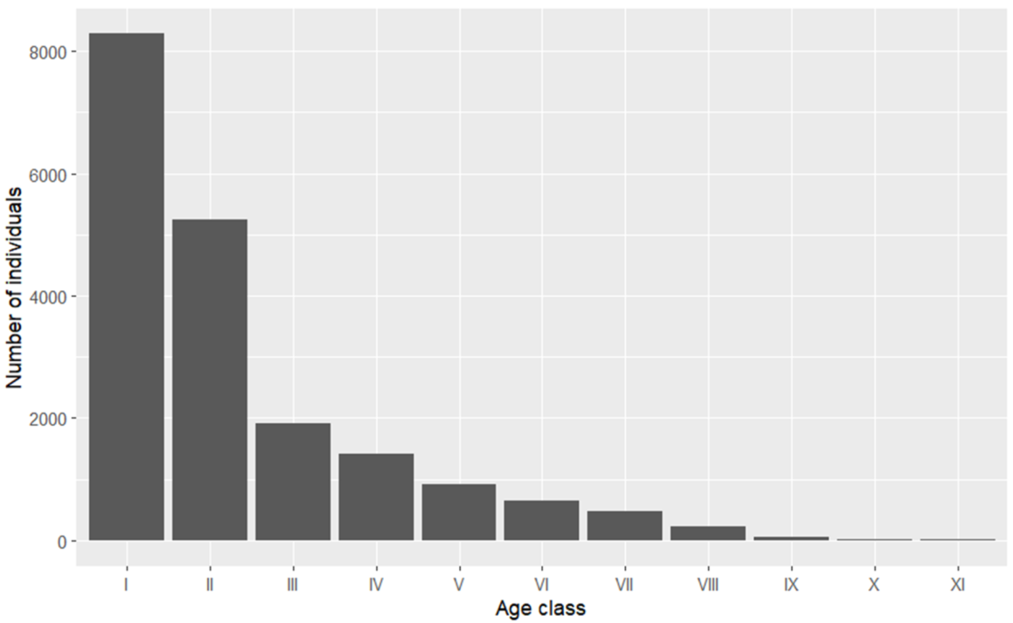
• number=c(8283,5238,1921,1425,926,659,479,228,57,24,10)
• Npop =Ntable(ax=number)

Taking the age class data in Table 1 as an example, we utilize the Ntable() function to organize the data into a data format (Npop, Table 4) that is suitable for population structure analysis. Here, a_x represents the number of tree individuals corresponding to each age class as the age class progresses.

Table 4. A standard data format that is suitable for population structure analysis.

Rank	Age Class	ax
1	I	8283
2	II	5238
3	III	1921
4	IV	1425
5	V	926
6	VI	659
7	VII	479
8	VIII	228
9	IX	57
10	X	24
11	XI	10

Note: a_x represents the number of tree individuals corresponding to each age class as the age class progresses.

• Step 3: Plot for population structure analysis.
• # Install.packages(“ggplot2”)
• library(ggplot2)
• fpop.p<-ggplot()+geom_bar(aes(x=rank,y=ax,group=ageclass),data=Npop,stat = “identity”)+
•  scale_x_continuous(breaks=1:11)+
•  scale_x_discrete(limits=Npop$ageclass)+
•  xlab(“Age class”)+ylab(“Number of individuals”)
• fpop.p

We employed the ggplot2 package to create the plot for the forest population structure (Figure 2). As the age advances, the number of individuals in this forest population gradually decreases. The age structure of the population presents an inverted “J”-shaped distribution, which clearly demonstrates that the population is a progressive one.

Figure 2. Plot for forest population structure.

• Step 4: Quantification of population dynamics.
• dyn(ax=Npop$ax)

We calculated the population dynamic index using the dyn() function, and the key results are presented in Table 5. The results demonstrate that the dynamic indices for each age class are all greater than 0, which indicates that the population can adapt effectively to the local environment and maintain relative stability over a certain period. When external disturbances are ignored, the dynamic index for the entire population $V_{pi}=42.999\%>0$, suggesting that the population is a growing population. When the influence of external disturbances is considered, $V_{pi}^{\prime }=0.391\%>0$, which is close to 0, indicating that the population shows a tendency of transition from a growing population to a stable one.

Table 5. Dynamic index quantification.

Age Class	I–II	II–III	III–IV	IV–V	V–VI	VI–VII	VII–VIII	VIII–IX	IX–X	X–XI	${\mathit{V}}_{\mathit{p}\mathit{i}}$	${\mathit{V}}_{\mathit{p}\mathit{i}}^{\prime }$
Dynamic Index Range	V1	V2	V3	V4	V5	V6	V7	V8	V9	V10
Dynamic index (%)	36.762	63.326	25.820	35.018	28.834	27.314	52.401	75.000	57.895	58.333	42.999	0.391

Note: V_n is the dynamic index of the individual number of the population from age class n to n + 1, $V_{pi}$ is the dynamic index of population change when external interference is ignored, and $V_{pi}^{\prime }$ is the dynamic index of population change when external interference is considered in the future.

• Step 5: Generate the static life table to analyze the population dynamic changes.
• lifetable(ax=Npop$ax)

We generated the life table by using the lifetable() function, and the key results are presented in Table 6.

Table 6. Life table compilation.

Age Class (x)	ax	lx	lnlx	dx	qx	Lx	Tx	ex	Kx	Sx
I	8283	1000	6.908	368	0.368	816	1824	1.825	0.459	0.632
II	5238	632	6.449	400	0.633	432	1008	1.596	1.002	0.367
III	1921	232	5.447	60	0.259	202	576	2.485	0.299	0.741
IV	1425	172	5.147	60	0.349	142	374	2.177	0.429	0.651
V	926	112	4.718	32	0.286	96	232	2.076	0.336	0.714
VI	659	80	4.382	22	0.275	69	136	1.706	0.322	0.725
VII	479	58	4.060	30	0.517	43	68	1.164	0.728	0.483
VIII	228	28	3.332	21	0.750	18	24	0.875	1.386	0.250
IX	57	7	1.946	4	0.571	5	7	1.000	0.847	0.429
X	24	3	1.099	2	0.667	2	2	0.667	1.099	0.333
XI	10	1	0.000	$-$	$-$	$-$	$-$	$-$	$-$	$-$

Note: x is the age class level, a_x is the number of individuals currently present within age class x, l_x is the standardized number of surviving individuals in age class x, d_x is the standardized number of deaths occurring between age classes x and x + 1, q_x is the mortality rate between age classes x and x + 1, L_x is the number of individuals who survive and transition from age class x to x + 1, T_x is the total number of individuals surviving from age class x onwards, e_x is the average expected remaining lifespan for individuals who have reached age class x, K_x is the population disappearance rate at age class x, and S_x is the x.

• Step 6: Regression analysis for survival curves.
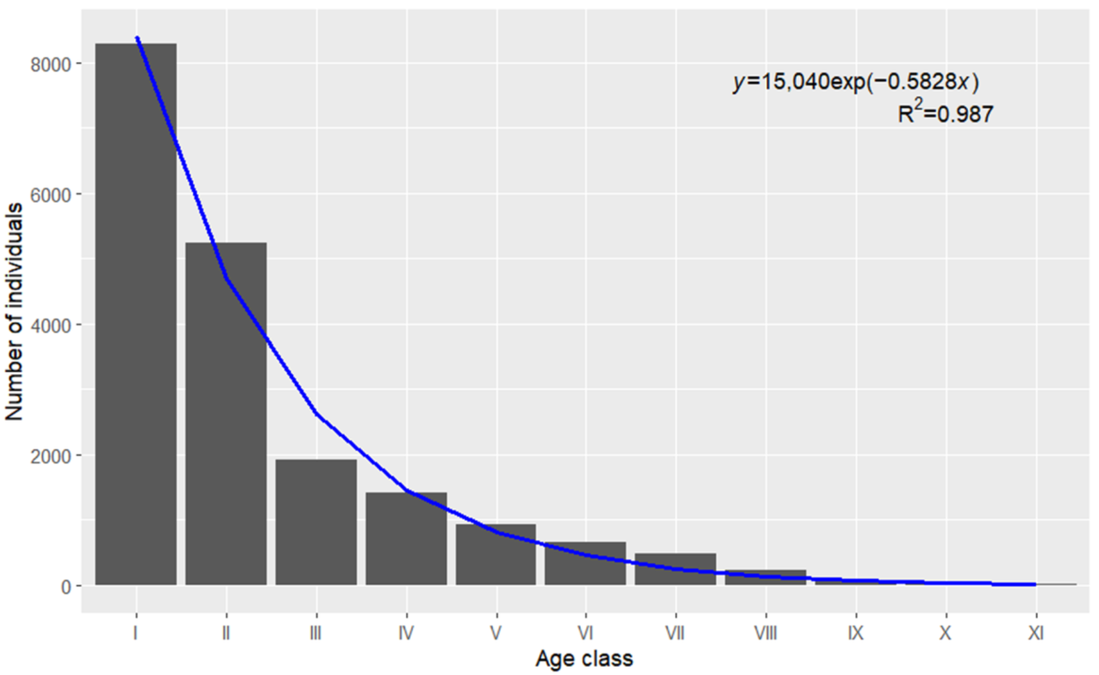
• psd_D1<-psdfun(ax=Npop$ax,index=“Deevey1”)
• psd_D1
• psd_D2<-psdfun(ax=Npop$ax,index=“Deevey2”)
• psd_D2
• psd_D3<-psdfun(ax=Npop$ax,index=“Deevey3”)
• psd_D3

The results of fitting the survival curve using the Deevey formulas were obtained by using the psdfun() function. The key results are presented in Table 7. These results suggest that among the three Deevey formulas, Deevey II yields the best fitting effect, with an R² value reaching 0.987.

Table 7. Deevey formulas for survival curve fitting.

Item	Formula	R2
Deevey I	y = 5603.9 – 642.3x	0.652
Deevey II	y = 15,040exp(–0.5828x)	0.987
Deevey III	y = 8691.1232x−1.2598	0.949

• Step 7: Plot for regression analysis of survival curves.
• # Install.packages(“ggplot2”)
• library(ggplot2)
• psdnls.p<-ggplot()+geom_bar(aes(x=age,y=ax,group=ageclass),data=psd_D2$Data,stat = “identity”)+
•  geom_line(aes(x=age,y=predict),color=“blue”,linewidth=1,data=psd_D2$Data)+
   geom_text(aes(x=9,y=7700),label=expression(paste(italic(y),”=15040exp(-0.5828”,italic(x),”)”)))+
•  geom_text(aes(x=10,y=7300),label=expression(paste(R^2,”=0.987”)))+
•  scale_x_continuous(breaks=1:11)+
   scale_x_discrete(limits=psd_D2$Data$ageclass)+
•  xlab(“Age class”)+ylab(“Number of individuals”)
• psdnls.p

We utilized the ggplot2 package to generate a plot for the regression analysis of survival curves (Figure 3). Meanwhile, the reshape2 package was employed to process the data. The results show that the Deevey II formula exhibits a satisfactory fitting effect.

Figure 3. Plot for regression analysis of survival curves.

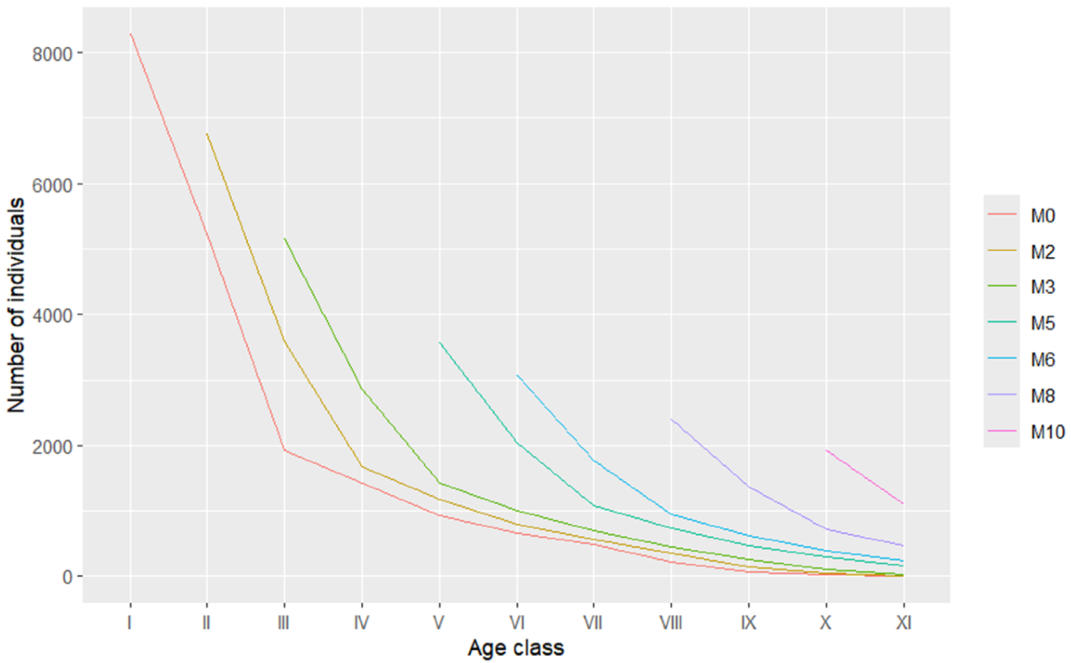
• Step 8: Time series prediction for the population dynamic changes.
• Mdata<-Mpre(ax=Npop$ax,n=c(2,3,5,6,8,10))
• # Install.packages(“reshape2”)
• library(reshape2)
• Mdata.melt<-reshape2::melt(Mdata,id=c(“rank”,”ageclass”))
• Mdata.melt$ageclass<-factor(Mdata.melt$ageclass,levels=unique(Mdata.melt$ageclass))
• # Install.packages(“ggplot2”)
• library(ggplot2)Mpre.p<-ggplot()+geom_line(aes(x=ageclass,y=value,color=variable,group=variable),
•  linewidth=0.5,data=Mdata.melt)+
•  xlab(“Age class”)+ylab(“Number of individuals”)+labs(color=“ “)
• Mpre.p

We predicted the time series by using the Mpre() function and generated a table and a figure for the time series prediction of the population dynamic changes (Table 8 and Figure 4). The results indicate that, in the prediction series, after time intervals corresponding to 2, 3, 5, 6, 8, and 10 age classes in the future, the peaks of the individual numbers in each age class of the population shift backward successively.

Table 8. Time series prediction of the population dynamic changes.

Rank	Age Class	M0 (ax)	M2	M3	M5	M6	M8	M10
1	I	8283
2	II	5238	6760
3	III	1921	3580	5147
4	IV	1425	1673	2861
5	V	926	1176	1424	3559
6	VI	659	792	1003	2034	3075
7	VII	479	569	688	1082	1775
8	VIII	228	354	455	743	940	2395
9	IX	57	142	255	470	629	1367
10	X	24	40	103	289	396	715	1924
11	XI	10	17	30	160	243	476	1097

Note: M0 is a_x and represents the number of tree individuals corresponding to each age class as the age class progresses; M2, M3, M5, M6, M8, and M10 represent the predicted values of the population size after 2, 3, 5, 6, 8 and 10 age classes, respectively.

Figure 4. Time series prediction of the population dynamic changes.

3.4. Presentation of a Comprehensive Case

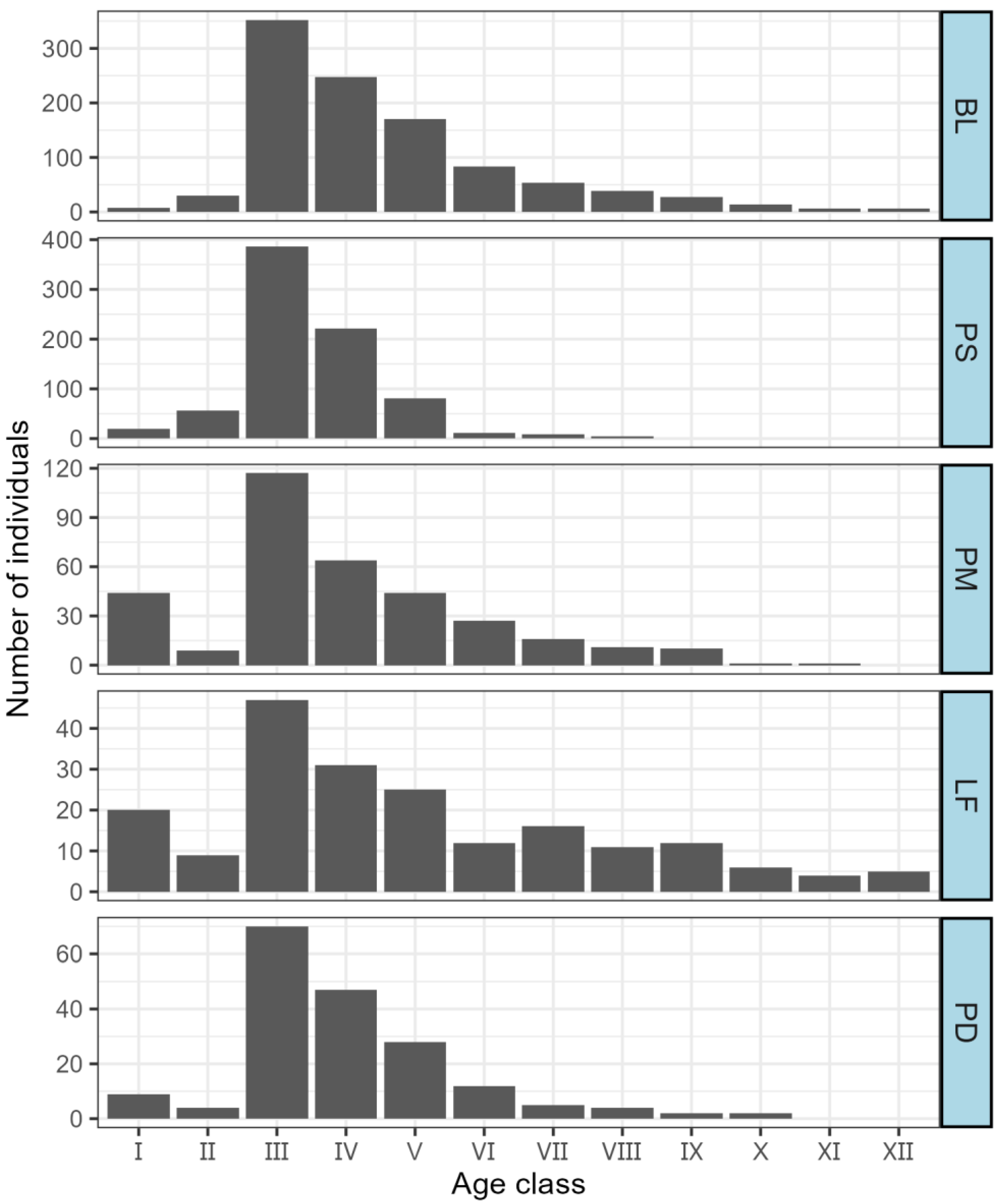
In this section, leveraging the data from our prior publication [13], we offer a comprehensive and in-depth demonstration of the research process related to the structure and numerical dynamics of forest populations. The study area was a secondary forest situated in a typical karst region of Guizhou Province, China. This forest has undergone more than 30 years of natural restoration after being abandoned. Through the establishment of representative sample plots and systematic vegetation surveys, we conducted a comparative analysis of the structural and numerical dynamic characteristics of five dominant populations. Our aim was to establish scientific theoretical underpinnings that can serve as reliable references for the protection and restoration of karst secondary forests. In this study, a total of 41 species and 3251 individuals of woody plants were surveyed. Among them, there were 1038 individuals of Betula luminifera (BL, accounting for 31.9%), 793 of Platycarya strobilacea (PS, 24.4%), 344 of Pinus massoniana (PM, 10.6%), 198 of Liquidambar formosana (LF, 6.1%), and 183 of Populus davidiana (PD, 5.6%). These five populations, with a combined total of 2556 individuals, constituted 78.6% of the surveyed plants and were identified as the dominant populations within the community. The age class data of these five dominant populations are presented in Table 9. The detailed criteria for age class division and relevant basic information are comprehensively elaborated in our published article [13]. Moreover, the R codes utilized in this section are available in the Supplementary File.

Table 9. Age class data of five dominant populations in typical karst secondary forests.

Rank	Diameter Class (cm)	Age Class	ax
			BL	PS	PM	LF	PD
1	(0,1)	I	8	20	44	20	9
2	[1,3)	II	30	57	9	9	4
3	[3,5)	III	352	386	117	47	70
4	[5,7)	IV	247	221	64	31	47
5	[7,9)	V	171	81	44	25	28
6	[9,11)	VI	83	12	27	12	12
s7	[11,13)	VII	54	9	16	16	5
8	[13,15)	VIII	39	4	11	11	4
9	[15,17)	IX	28	1	10	12	2
10	[17,19)	X	14	1	1	6	2
11	[19,21)	XI	6	1	1	4	—
12	[21,$\infty$)	XII	6	—	—	5	—

Note: BL is Betula luminifera, PS is Platycarya strobilacea, PM is Pinus massoniana, LF is Liquidambar formosana, and PD is Populus davidiana. a_x represents the number of tree individuals corresponding to each age class as the age class progresses.

As depicted in Figure 5, the age class structures of the five dominant populations are relatively comprehensive. In general, for each population, the number of individuals exhibits a unimodal pattern, initially rising and subsequently declining as the age class advances. Nevertheless, owing to the relatively scarce number of individuals in age classes I—II of each dominant population and the substantial fluctuations observed in these early age classes, there is an overall deficiency in population renewal. This ultimately leads to suboptimal population stability.

Figure 5. Age class structure of five dominant populations in typical karst secondary forests.

The dynamic indices show (Table 10) that the numeric dynamics of the five dominant populations all exhibit a trend of first decline and then growth. The overall dynamic indices V_pi and V′_pi of the five dominant populations are both greater than zero, indicating that the five dominant populations are generally in a growth trend. The growth potential is ranked as PM > PS > PD > BL > LF. When affected by the external environment, the Pinus massoniana population has the highest probability of being disturbed, while the Betula luminifera population has the lowest. In addition, the insufficient number of individuals in age classes I, II may hinder the stable and sustainable development of the population.

Table 10. Dynamic index of five dominant populations in typical karst secondary forests.

Age Class	Dynamic Index Class	Dynamic Index (%)
		BL	PS	PM	LF	PD
I–II	V1	−73.333	−64.912	79.545	55.000	55.556
II–III	V2	−91.477	−85.233	−92.308	−80.851	−94.286
III–IV	V3	29.830	42.746	45.299	34.043	32.857
IV–V	V4	30.769	63.348	31.250	19.355	40.426
V–VI	V5	51.462	85.185	38.636	52.000	57.143
VI–VII	V6	34.940	25.000	40.741	−25.000	58.333
VII–VIII	V7	27.778	55.556	31.250	31.250	20.000
VIII–IX	V8	28.205	75.000	9.091	−8.333	50.000
IX–X	V9	50.000	0.000	90.000	50.000	0.000
X–XI	V10	57.143	0.000	0.000	33.333	-
XI–XII	V11	0.000	-	-	−20.000	-
Vpi		30.299	40.838	41.601	24.356	38.248
V′pi		0.421	3.713	3.782	0.507	1.912
Pmax		1.389	9.091	9.091	2.083	5.000

Through the compilation of static life tables for the five dominant populations (Table 11), it becomes feasible to ascertain the survival status of different populations across various growth stages. This approach allows for a comprehensive understanding of the competitive relationships among populations and a clear elucidation of the disparities in aspects such as resource acquisition and space occupation. Consequently, it offers vital information for the study of niche differentiation within the community and the dynamic development of populations.

Table 11. Static life tables of five dominant populations in typical karst secondary forests.

Population	Age Class (x)	ax	a′x	lx	lnlx	dx	qx	Lx	Tx	ex	Kx	Sx
BL	I	8	420	1000	6.908	117	0.117	942	3757	3.757	0.124	0.883
	II	30	371	883	6.783	45	0.051	860	2816	3.189	0.052	0.949
	III	352	352	838	6.731	250	0.298	713	1955	2.333	0.354	0.702
	IV	247	247	588	6.377	181	0.308	498	1242	2.112	0.368	0.692
	V	171	171	407	6.009	209	0.514	302	744	1.829	0.721	0.486
	VI	83	83	198	5.288	69	0.348	164	442	2.232	0.428	0.652
	VII	54	54	129	4.860	36	0.279	111	278	2.159	0.327	0.721
	VIII	39	39	93	4.533	26	0.280	80	168	1.801	0.328	0.720
	IX	28	28	67	4.205	34	0.507	50	88	1.306	0.708	0.493
	X	14	14	33	3.497	19	0.576	24	38	1.136	0.857	0.424
	XI	6	6	14	2.639	0	0.000	14	14	1.000	0.000	1.000
	XII	6	6	14	2.639	$-$	$-$	$-$	$-$	$-$	$-$	$-$
PS	I	20	550	1000	6.908	211	0.211	894	2590	2.590	0.237	0.789
	II	57	434	789	6.671	87	0.110	746	1696	2.149	0.117	0.890
	III	386	386	702	6.554	300	0.427	552	950	1.353	0.557	0.573
	IV	221	221	402	5.996	255	0.634	274	398	0.990	1.006	0.366
	V	81	81	147	4.990	125	0.850	84	124	0.840	1.899	0.150
	VI	12	12	22	3.091	6	0.273	19	39	1.773	0.318	0.727
	VII	9	9	16	2.773	9	0.563	12	20	1.250	0.827	0.438
	VIII	4	4	7	1.946	5	0.714	4	8	1.214	1.253	0.286
	IX	1	1	2	0.693	0	0.000	2	4	2.000	0.000	1.000
	X	1	1	2	0.693	0	0.000	2	2	1.000	0.000	1.000
	XI	1	1	2	0.693	$-$	$-$	$-$	$-$	$-$	$-$	$-$
PM	I	44	265	1000	6.908	309	0.309	846	2289	2.289	0.370	0.691
	II	9	183	691	6.538	249	0.360	566	1444	2.089	0.447	0.640
	III	117	117	442	6.091	200	0.452	342	877	1.984	0.602	0.548
	IV	64	64	242	5.489	76	0.314	204	535	2.211	0.377	0.686
	V	44	44	166	5.112	64	0.386	134	331	1.994	0.487	0.614
	VI	27	27	102	4.625	42	0.412	81	197	1.931	0.531	0.588
	VII	16	16	60	4.094	18	0.300	51	116	1.933	0.357	0.700
	VIII	11	11	42	3.738	4	0.095	40	65	1.548	0.100	0.905
	IX	10	10	38	3.638	34	0.895	21	25	0.658	2.251	0.105
	X	1	1	4	1.386	0	0.000	4	4	1.000	0.000	1.000
	XI	1	1	4	1.386	$-$	$-$	$-$	$-$	$-$	$-$	$-$
LF	I	20	65	1000	6.908	200	0.200	900	3862	3.863	0.223	0.800
	II	9	52	800	6.685	77	0.096	762	2962	3.703	0.101	0.904
	III	47	47	723	6.583	246	0.340	600	2201	3.044	0.416	0.660
	IV	31	31	477	6.168	92	0.193	431	1601	3.356	0.214	0.807
	V	25	25	385	5.953	200	0.519	285	1170	3.039	0.733	0.481
	VI	12	12	185	5.220	−61	−0.330	216	885	4.784	−0.285	1.330
	VII	16	16	246	5.505	77	0.313	208	670	2.722	0.375	0.687
	VIII	11	11	169	5.130	−16	−0.095	177	462	2.734	−0.090	1.095
	IX	12	12	185	5.220	93	0.503	138	285	1.541	0.699	0.497
	X	6	6	92	4.522	30	0.326	77	146	1.592	0.395	0.674
	XI	4	4	62	4.127	−15	−0.242	70	70	1.121	−0.217	1.242
	XII	5	5	77	4.344	$-$	$-$	$-$	$-$	$-$	$-$	$-$
PD	I	9	90	1000	6.908	200	0.200	900	3177	3.177	0.223	0.800
	II	4	72	800	6.685	22	0.028	789	2277	2.846	0.028	0.973
	III	70	70	778	6.657	256	0.329	650	1488	1.913	0.399	0.671
	IV	47	47	522	6.258	211	0.404	416	838	1.605	0.518	0.596
	V	28	28	311	5.740	178	0.572	222	422	1.355	0.849	0.428
	VI	12	12	133	4.890	77	0.579	94	200	1.500	0.865	0.421
	VII	5	5	56	4.025	12	0.214	50	105	1.875	0.241	0.786
	VIII	4	4	44	3.784	22	0.500	33	55	1.250	0.693	0.500
	IX	2	2	22	3.091	0	0.000	22	22	1.000	0.000	1.000
	X	2	2	22	3.091	$-$	$-$	$-$	$-$	$-$	$-$	$-$

Note: a′_x is a_x after smoothing treatment; the other codes are shown in the “NOTE” of Table 6.

The results of fitting the survival curves of the five dominant populations (Table 12) indicate that, among the three Deevey formulas, the Deevey II formula yields the best fitting effect, with a larger R² value. Evidently, the survival curves of the five dominant populations are all closer to the Deevey II type.

Table 12. Deevey formulas for survival curve fitting of five dominant populations in typical karst secondary forests.

Population	Item	Formula	R2
BL	Deevey I	y = 415.7270 − 40.9970x	0.880
	Deevey II	y = 623.2204exp(0.2771x)	0.941
	Deevey III	y = 495.4938x0.7931	0.767
PS	Deevey I	y = 489.3450 − 55.800x	0.791
	Deevey II	y = 886.5610exp(0.3894x)	0.937
	Deevey III	y = 621.1776x0.9915	0.800
PM	Deevey I	y = 203.7090 − 22.7550x	0.759
	Deevey II	y = 421.3343exp(0.4433x)	0.997
	Deevey III	y = 284.3897x1.0767	0.927
LF	Deevey I	y = 58.1970 − 5.2867x	0.860
	Deevey II	y = 86.2053exp(0.2513x)	0.976
	Deevey III	y = 72.7050x0.749	0.867
PD	Deevey I	y = 91.6670 − 10.6300x	0.901
	Deevey II	y = 134.4295exp(0.3139x)	0.933
	Deevey III	y = 102.3071x0.8303	0.777

Note: y is a′_x in Table 11.

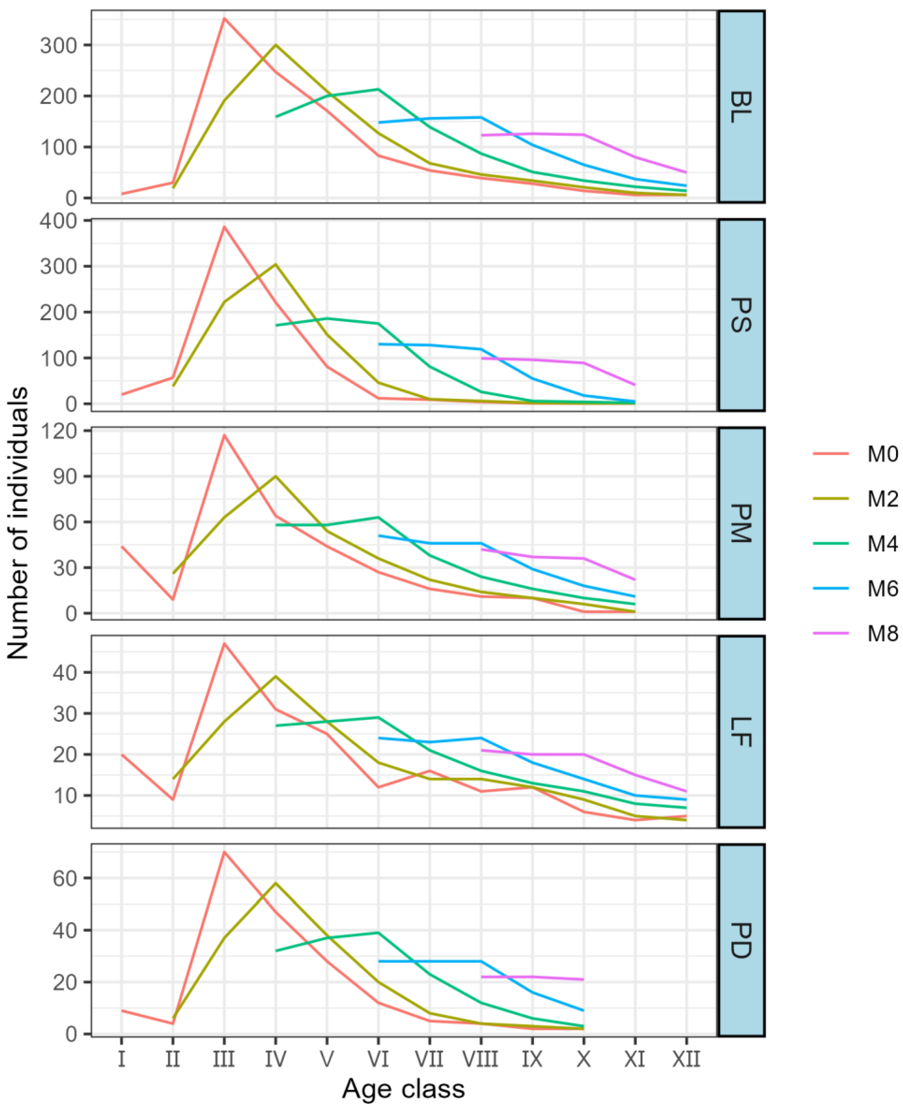
The time series prediction results indicate (Figure 6) that the five dominant populations exhibit roughly the same trend. Specifically, the population size experiences a sharp decline in the early stage and then a stable increase in the later stage. In the future age classes, the advantage in the number of individuals in each dominant population weakens. Subsequently, as the age class increases, the decline in the number of individuals gradually disappears and then shows an increasing trend. The most significant increase in the number of individuals occurs in the VI age class. After six age classes, the structures of various populations gradually become more reasonable, presenting a stable growth trend.

Figure 6. Time series prediction of five dominant populations in typical karst secondary forests.

In summary, notable disparities exist in the structure and numerical dynamics of the five dominant populations. Nevertheless, overall, they display a stable growth tendency. The limited number of individuals in the I–II age classes stands out as the primary factor impeding the stable development of the populations. It is advisable to improve the stand quality and the quantity of regeneration through a combination of enclosure protection and artificial tending measures. This integrated approach is expected to foster the stable and sustainable development of the secondary forest community.

3.5. Comparison with Other R Packages Used for Plant Population Structure Analysis

In the realm of plant population structure and numeric dynamics research, various software packages offer distinct forms of support for research endeavors. R packages, including poppr, popbio, ecostats, and TreeSim, each possess unique characteristics and application limitations (Table 13). When compared to other software, forestPSD stands out with remarkable advantages in the research of forest population structure and quantitative dynamics. It can directly and efficiently analyze the structure and numeric dynamics of forest tree populations. The generated visualizations and calculated indices can intuitively and accurately represent the characteristics of forest populations, thereby offering clear directions for research. Leveraging the R language, forestPSD exhibits high expandability and flexibility. This enables researchers to conduct customized development in accordance with the actual requirements of their research, thus catering to a wide range of complex research scenarios. Consequently, it serves as an indispensable tool for forest researchers engaged in relevant studies.

Table 13. Comparison with other R packages used for plant population structure analysis.

R Package	Description	Citation
forestPSD	forestPSD encompasses quantitative analyses of population changes, age structure, life tables, and population dynamics within specific spatial and temporal frameworks. This package provides researchers with an efficient and user-friendly instrument for analyzing forest population structures and their temporal alterations.	[14]
poppr	poppr mainly focuses on processing population genetic data with repeated measurements and has advantages in the analysis of plant population genetic structure and dynamics. It can help researchers understand the genetic diversity and evolutionary history of plant populations and provide information for population structure and quantity dynamics research from a genetic perspective. However, its application scope is relatively narrow, only suitable for the analysis of specific genetic data, and it has difficulties meeting the needs of a comprehensive analysis of plant populations with multiple factors. It cannot effectively analyze the impact of non-genetic factors on population structure and quantity dynamics.	[15]
popbio	popbio is good at predicting the long-term dynamic changes in populations. In the research of plant population quantity dynamics, it can simulate the development process of plant populations under different environmental conditions, calculate key indicators such as the population growth rate and extinction probability, and provide a reference basis for the management and protection of plant populations. But when dealing with the impact of complex multi-species interactions and spatial structure relationships on plant population structure and quantity dynamics, its analysis ability is slightly insufficient.	[16]
ecostats	ecostats provides a wealth of ecological statistical analysis tools. It can calculate community diversity indices, analyze species richness, etc., helping researchers understand the structure and dynamic changes in plant communities from multiple perspectives. It can also explore the key factors affecting plant population structure and quantity dynamics through correlation analysis and other methods. However, it requires users to have a high level of statistical knowledge. It may be difficult for researchers with a weak statistical foundation to use, and its running speed is slow when processing large-scale data.	[17]
TreeSim	TreeSim can simulate and generate evolutionary trees, helping researchers understand the evolutionary relationships and phylogenetic history of plant species and providing certain references for plant population structure and quantity dynamics research from an evolutionary perspective. But when analyzing the plant population structure and quantity dynamics that have nothing to do with evolutionary trees, its functions are relatively weak, and the application scenarios are relatively limited.	[18]

4. Conclusions

In response to the increasing complexity of ecological research, our newly developed forestPSD package presents an innovative and robust approach to studying forest population structure and dynamics. This user-friendly package enables researchers to generate comprehensive ecological analyses through sophisticated built-in algorithms by simply inputting standardized data. It serves as a powerful analytical framework for investigating forest population conservation mechanisms and developing evidence-based management strategies. The forestPSD package demonstrates several notable advantages over conventional methodologies, including enhanced data processing capabilities, streamlined model fitting procedures, and superior visualization functionality. These features facilitate deeper insights into data distribution patterns and temporal trends, thereby improving analytical efficiency and providing reliable empirical evidence for subsequent research and policy decisions. Moreover, our study offers detailed technical guidelines and case analyses, which can help researchers conduct rapid and efficient analyses of forest population structure and numeric dynamics. Moving forward, we are committed to enhancing the forestPSD package through continuous development. Our future improvements will focus on two key aspects: functional expansion and performance optimization. In terms of functionality, we plan to incorporate advanced ecological analysis methods and models to address population dynamics across diverse ecosystems, species characteristics, and research contexts. Regarding performance, we will substantially enhance the package’s computational efficiency and stability through algorithmic optimization and improved data management systems, ensuring robust performance when handling large-scale datasets. Through these systematic improvements, the forestPSD package will evolve into a more comprehensive, precise, and practical analytical tool for forest population research, contributing significantly to the advancement of population ecology.

References

- Zhang, Y.; Wang, J.; Wang, X.; Wang, L.; Wang, Y.; Wei, J.; Niu, Z.; Jian, L.; Jin, B.; Chen, C.; et al. Population Structures and Dynamics of Rhododendron Communities with Different Stages of Succession in Northwest Guizhou, China. Plants 2024, 13, 946. [Google Scholar] [CrossRef] [PubMed]
- Farahat, E.A. Age structure and static life tables of the endangered Juniperus phoenicea L. in North Sinai Mountains, Egypt: Implication for conservation. J. Mt. Sci. 2020, 17, 2170–2178. [Google Scholar] [CrossRef]
- Sigasa, M.N.; Yessoufou, K.; Magadlela, A.; Otang-Mbeng, W.; Suinyuy, T.N. Population Structure of an African Cycad: Fire May Stimulate the Coning Phenology of Encephalartos lanatus (Zamiaceae) and Also Predispose Its Cones to Damage. Diversity 2023, 15, 1075. [Google Scholar] [CrossRef]
- Huang, D.; Ren, Y.; Yang, S.; Zhao, Y.; Zhao, G. Population Structure and Dynamic Characteristics of Three Endemic Chinese Abies Species in Southeastern Tibet, China. Front. Ecol. Evol. 2024, 12, 1487984. [Google Scholar] [CrossRef]
- Yuan, G.; Guo, Q.; Xie, N.; Zhang, Y.; Luo, S.; Gui, Q.; Yao, S. Population Dynamics and Protection Strategies of Litsea coreana Levl. var. sinensis with Guizhou Province in China as an Example. J. Mt. Sci. 2023, 20, 1090–1101. [Google Scholar]
- Zabek, M.A.; Berman, D.M.; Blomberg, S.P.; Collins, C.W.; Wright, J. Population Dynamics of Feral Horses (Equus caballus) in an Exotic Coniferous Plantation in Australia. Wildl. Res. 2016, 43, 358–367. [Google Scholar] [CrossRef]
- Watkinson, A.R.; Powell, J.C. The Life History and Population Structure of Cycas armstrongii in Monsoonal Northern Australia. Oecologia 1997, 111, 341–349. [Google Scholar] [CrossRef] [PubMed]
- Li, W.; Zhang, G. Population Structure and Spatial Pattern of the Endemic and Endangered Subtropical Tree Parrotia subaequalis (Hamamelidaceae). Flora 2015, 212, 10–18. [Google Scholar] [CrossRef]
- Kang, D.; Guo, Y.; Ren, C.; Zhao, F.; Feng, Y.; Han, X.; Yang, G. Population Structure and Spatial Pattern of Main Tree Species in Secondary Betula platyphylla Forest in Ziwuling Mountains, China. Sci. Rep. 2014, 4, 6873. [Google Scholar] [CrossRef] [PubMed]
- Deevey, E.S. Life Tables for Natural Populations of Animals. Q. Rev. Biol. 1947, 22, 283–314. [Google Scholar] [CrossRef] [PubMed]
- Peng, C.; Ai, W.; Qi, L.; Tu, J.; Meng, Y.; Yang, M.; Li, M. Cunninghamia lanceolata Sprout Population Structure, Dynamics and Biomass Allocation Changes During Phyllostachys Edulis Expansion in Middleo-Southern China. Trees-Struct. Funct. 2022, 36, 1207–1218. [Google Scholar] [CrossRef]
- Liu, D.; Guo, Z.; Cui, X.; Fan, C. Estimation of the Population Dynamics of Taxus cuspidata by Using a Static Life Table for Its Conservation. Forests 2023, 14, 2194. [Google Scholar] [CrossRef]
- Wei, H.; Xu, M.; Chai, Z.; Sun, C. Population Structure and Numeric Dynamic of Dominant Species of Karst Secondary Forests. J. Northeast For. Univ. 2023, 51, 80–85. [Google Scholar]
- Chai, Z. forestPSD: Forest Population Structure and Numeric Dynamics; R Package Version 1.0.0; R Foundation for Statistical Computing: Vienna, Austria, 2024. [Google Scholar]
- Zhian, N. Poppr: Genetic Analysis of Populations with Mixed Reproduction; R Package Version 2.9.6; R Foundation for Statistical Computing: Vienna, Austria, 2024. [Google Scholar]
- Chris, S.; Brook, M.; Patrick, N. Popbio: Construction and Analysis of Matrix Population Models; R Package Version 2.8; R Foundation for Statistical Computing: Vienna, Austria, 2024. [Google Scholar]
- David, W.; Christopher, C.; Mark, D.; Eve, S. Ecostats: Code and Data Accompanying the Eco-Stats Text (Warton 2022); R Package Version 1.2.1; R Foundation for Statistical Computing: Vienna, Austria, 2024. [Google Scholar]
- Tanja, S. TreeSim: Simulating Phylogenetic Trees; R Package Version 2.4; R Foundation for Statistical Computing: Vienna, Austria, 2024. [Google Scholar]
Disclaimer/Publisher’s Note: The statements, opinions and data contained in all publications are solely those of the individual author(s) and contributor(s) and not of MDPI and/or the editor(s). MDPI and/or the editor(s) disclaim responsibility for any injury to people or property resulting from any ideas, methods, instructions or products referred to in the content. |
© 2025 by the authors. Licensee MDPI, Basel, Switzerland. This article is an open access article distributed under the terms and conditions of the Creative Commons Attribution (CC BY) license (https://creativecommons.org/licenses/by/4.0/).