FPGA-Accelerated Lightweight CNN in Forest Fire Recognition

Abstract

Using convolutional neural networks (CNNs) to recognize forest fires in complex outdoor environments is a hot research direction in the field of intelligent forest fire recognition. Due to the storage-intensive and computing-intensive characteristics of CNN algorithms, it is difficult to implement them at edge terminals with limited memory and computing resources. This paper uses a FPGA (Field-Programmable Gate Array) to accelerate CNNs to realize forest fire recognition in the field environment and solves the problem of the difficulty in giving consideration to the accuracy and speed of a forest fire recognition network in the implementation of edge terminal equipment. First, a simple seven-layer lightweight network, LightFireNet, is designed. The network is compressed using a knowledge distillation method and the classical network ResNet50 is used as the teacher network to supervise the learning of LightFireNet so that its accuracy rate reaches 97.60%. Compared with ResNet50, the scale of LightFireNet is significantly reduced. Its model parameter amount is 24 K and its calculation amount is 9.11 M, which are 0.1% and 1.2% of ResNet50, respectively. Secondly, the hardware acceleration circuit of LightFireNet is designed and implemented based on the FPGA development board ZYNQ Z7-Lite 7020. In order to further compress the network and speed up the forest fire recognition circuit, the following three methods are used to optimize the circuit: (1) the network convolution layer adopts a depthwise separable convolution structure; (2) the BN (batch normalization) layer is fused with the upper layer (or full connection layer); (3) half float or ap_fixed<16,6>-type data is used to express feature data and model parameters. After the circuit function is realized, the LightFireNet terminal circuit is obtained through the circuit parallel optimization method of loop tiling, ping-pong operation, and multi-channel data transmission. Finally, it is verified on the test dataset that the accuracy of the forest fire recognition of the FPGA edge terminal of the LightFireNet model is 96.70%, the recognition speed is 64 ms per frame, and the power consumption is 2.23 W. The results show that this paper has realized a low-power-consumption, high-accuracy, and fast forest fire recognition terminal, which can thus be better applied to forest fire monitoring.

1. Introduction

Forest fires cause serious damage to ecosystems and infrastructure and also cause casualties. Forest fire monitoring can help people find and extinguish fires in the early stages of a fire, prevent the spread of a fire, and greatly reduce the cost and loss of firefighting [1]. Early forest fire monitoring methods mainly rely on manual patrols, observation posts, and manual alarms. These methods are simple to operate but the monitoring scope is limited, and there are risks of response delays and false alarms [2]. At the end of the 20th century and the beginning of the 21st century, fire monitoring technology based on computer vision began to be studied. Fire monitoring methods based on computer vision can be divided into traditional image processing-based methods and deep learning-based methods [3]. Traditional image processing methods are mainly based on three features: color [4], motion [5], and geometric features [6,7]. The above methods based on color, motion, and geometric features have the problems of low accuracy, high false alarm rate, and the inability to detect long-distance or small-scale fires. In addition, image processing methods require a lot of prior knowledge, complex feature engineering, and tedious operations, and the robustness of the models is poor.

In recent years, CNNs based on deep learning have achieved good results in image classification and target monitoring [8]. Different from the traditional fire monitoring technology based on image processing, CNNs can automatically extract and learn complex features, reducing the need for manual feature engineering. At present, many CNNs have been applied to fire monitoring tasks, and significant progress has been made in improving detection accuracy [9]. Khan et al. [10] proposed a forest fire detection method, FFireNet, based on deep learning. This method uses a MobileNetV2 pre-training convolution layer and adds a full connection layer to achieve a classification accuracy of 97.42%, which is excellent in fire and non-fire image classification. While this approach benefits from MobileNetV2’s efficient depthwise separable convolutions, its reliance on the full MobileNetV2 backbone results in relatively high computational complexity, making real-time execution challenging on resource-constrained edge devices. Moreover, the study focused solely on binary fire/non-fire classification, limiting its applicability in scenarios requiring smoke detection—a critical feature for early forest fire warning systems. Peng et al. [11] proposed a smoke monitoring algorithm combining manual features and deep learning features, which can distinguish smoke from non-smoke, which is easily confused, and achieved an accuracy of 97.12% in the test set. The hybrid design enhances interpretability through manual features while maintaining the representational power of deep learning. However, the manual feature engineering component increases development complexity and may lack adaptability to new environments. Additionally, the computational overhead of extracting dual feature sets limits real-time performance, making it impractical for large-scale sensor networks. Zhang et al. [12] proposed an ATT Squeeze U-Net based on U-Net and SqueezeNet, achieving 93% recognition accuracy. The attention modules effectively highlight fire-related regions while suppressing background interference. However, the accuracy remains lower than other contemporary approaches, particularly in challenging scenarios with small or occluded fire regions. Compared with the early fire monitoring method, the fire monitoring method based on CNNs has higher accuracy and robustness, especially suitable for dealing with complex forest fire scenarios.

Although CNNs are considered to be the best model for monitoring forest fire events [13], their computing-intensive and memory-intensive characteristics limit their direct deployment on edge devices with limited resources. Most CNN-based forest fire monitoring systems have high hardware requirements [14]. Currently, most CNN-based fire monitoring systems adopt an “edge collection + cloud computing” approach, where edge devices collect fire images and transmit data to cloud servers for analysis and recognition [15]. The literature [16] points out that if a large number of edge devices are added, a large amount of terminal data will be transmitted to the cloud for processing, and the data transmission performance will be reduced, eventually leading to a significant increase in data transmission delay and energy consumption. Edge cloud architecture makes use of the powerful computing power of the cloud and can handle complex CNN models. However, because the forest fire monitoring environment is a field with poor network conditions, the delay of data transmissions and the uncontrollability of the network will lead to the reduced recognition effect. In addition to the “edge cloud architecture”, Ref. [17] also proposed another edge deployment scheme for CNNs, that is, using UAVs (Unmanned Aerial Vehicles) to deploy CNNs. The reason why the UAV can realize CNN edge computing is that the UAV is equipped with a high-performance processor, and the CNN algorithm can be directly deployed on the UAV platform, which solves the above problems of CNN deployment. However, this scheme is expensive, not suitable for promotion, and cannot achieve intensive deployment. It is only suitable for fire monitoring after fire detection and cannot achieve long-term monitoring effects. Therefore, research on how to use a CNN forest fire monitoring algorithm to quickly execute in low-cost, performance-constrained edge terminals is the key to promoting the application of a CNN model in forest fire monitoring.

The key to deploying the CNN model in resource-constrained edge devices is to design lightweight CNNs. In recent years, more and more lightweight networks have been explored, such as MobileNet [18], SqueezeNet [19], and ShuffleNet [20]. Almida et al. [21] proposed a new lightweight CNN model EdgeFireSmoke, which can detect wildfires through RGB (red, green, blue) images and can be used to monitor wildfires through aerial images of UAVs (Unmanned Aerial Vehicles) and video surveillance systems. The classification time is about 30 ms per frame, and the accuracy rate is 98.97%. Wang et al. [22] proposed a lightweight fire detection algorithm based on the improved Pruned + KD model, which has the advantages of fewer model parameters, low memory requirements, and fast reasoning speed.

In addition to lightweight model design, hardware acceleration is also an effective way to solve the bottleneck of CNN computing. As a common hardware acceleration device, GPU has strong parallel computing capability, which can significantly improve the speed of fire recognition. However, the high power consumption and high cost of GPU limit its application in long-term field monitoring. In contrast, FPGA, with its advantages of low power consumption, small size, and high customizability, has gradually become an ideal choice for accelerating CNNs in edge environments [23]. FPGA can optimize the calculation process of CNNs through a hardware circuit, realize high parallel calculation, and achieve an acceleration effect close to GPU under low power consumption [24]. Although FPGA acceleration technology has significant advantages, it also faces the challenge of resource constraints. Due to the limited resources in a FPGA chip, the ability of a single FPGA to accelerate a complex CNN model is limited, and the model design needs to make trade-offs between resource allocation and optimization. Therefore, we have to simplify the model or adopt a more efficient hardware design to ensure that the model can run normally on an FPGA and achieve the expected performance goals.

To address these challenges, we propose a FPGA-accelerated lightweight CNN framework for forest fire recognition. Our solution combines two key innovations: (1) a compact network architecture designed with hardware efficiency in mind, leveraging depthwise separable convolution and knowledge distillation to maintain accuracy while minimizing computational complexity; (2) a hardware–software co-design approach that optimizes the FPGA implementation through parallel computing strategies (e.g., a loop tiling ping-pong buffer) and memory access optimization.

The main contributions of this work include:

• A novel lightweight CNN model tailored for edge deployment in forest fire monitoring.
• An optimized FPGA acceleration framework that bridges the gap between algorithmic efficiency and hardware constraints.
• Comprehensive evaluation comparing the proposed system with alternative computing platforms.

The remainder of this paper is organized as follows: Section 2 describes the materials and methodology, Section 3 presents the experimental results, and Section 4 discusses the implications and future work.

2. Materials and Methods

2.1. System Structure

Figure 1 shows the FPGA development board structure. We have adopted an integrated edge device architecture, which takes the Zynq Z7 Lite 7020 SoC development board as the core (as shown in Figure 1), supplemented by a camera module and LCD display module. As the core of the development board, the Zynq7020 chip is composed of a processing system (PS side) and a programmable logic module (PL side) composed of two ARM Cortex-A9 processors. The two components (PS and PL) closely cooperate through the high-speed AXI (Advanced eXtensible Interface) bus to achieve efficient collaboration between software and hardware. The PS terminal is responsible for loading LightFireNet parameters, processing characteristic data, displaying recognition results, and controlling the entire recognition process. The PL terminal focuses on image acquisition and provides hardware acceleration support for LightFireNet. We chose the OV5640 CMOS camera to capture images. The camera is connected to the PL end, and the image data are transmitted to the DDR3 memory of the PS end through the AXI VDMA interface for LightFireNet processing. The network parameters are stored on the SD card. When the system starts, the ARM processor on the PS side reads these parameters from the SD card to the memory. Finally, the ARM system on the PS side is responsible for transmitting image data and network parameters to the LightFireNet on the PL side, controlling the operation of the accelerator, and displaying the fire recognition results on the LCD screen in real-time.

As shown in Figure 2, during the startup of the forest fire recognition system, the system first performs power-on initialization. Subsequently, the ARM processor reads the LightFireNet model parameters from the SD card to the DRAM. The PL terminal hardware circuit starts; the camera and VDMA module complete the initialization configuration, start capturing RGB images, and transmit data to DRAM through DMA. The ARM processor on the PS side performs the image scaling and normalization preprocessing and then sends the preprocessed image data and model parameters to the PL side. The LightFireNet acceleration circuit on the PL side calculates and returns the result to the PS side through the AXI bus. The ARM processor superimposes the detection results on the collected images and displays the final results through the HDMI display. This system process is automatic and efficient, ensuring real-time and accurate fire detection.

2.2. Forest Fire Recognition Model Design

2.2.1. Dataset and Pre-Processing

To better simulate the complex background environment of forest fires, images with intricate backgrounds were selected from the Kaggle dataset website to construct a dataset containing three types of samples: fire, non-fire, and smoke, totaling 5553 images. These images cover various scenarios, including forest fires, natural states of forests without fire, and smoke in forests. Additionally, to train a more robust model, the dataset also includes complex samples such as fire clouds, white clouds, and red-leaf forests. Figure 3 shows pictures of some typical datasets: (a) depicts fire images, including small and large fires; (b) shows no-fire images, including fire clouds, red-leaf forests, and clouds resembling smoke; (c) displays smoke images, including light and heavy smoke. This dataset provides comprehensive coverage of various forest fire scenarios, offering rich samples for model training and evaluation. It is worth emphasizing that the effectiveness of the above data enhancement technology needs to be verified by the actual training effect. The experimental results in Section 3.2 and Section 3.3 in this paper show that the data enhancement technology can effectively solve the problem of imbalanced categories of existing datasets. In addition, the preprocessing part comprised four key steps: data cleaning, data augmentation, standardization, and stratified splitting. Each step was designed to enhance data quality, address class imbalance, and ensure compatibility with hardware constraints.

Prior to augmentation, all images were manually inspected to remove duplicates, low-quality samples (e.g., blurred or overexposed images), and irrelevant scenes (e.g., urban fires or indoor smoke). This step ensured that the dataset exclusively represented forest fire scenarios.

As shown in

Table 1. Dataset details.

Category	Number of Images
	Before Augmentation	After Augmentation
fire	2007	2496
non-fire	2579	3035
smoke	967	3028

, the category distribution of the original dataset is obviously unbalanced, and the number of fire and non-fire samples is significantly more than smoke samples. To reduce the negative impact of the uneven distribution on model training and enhance the model’s generalization ability in complex environments, we performed several data augmentation operations on the original dataset. Specifically, (a) the scene changes under different shooting angles were simulated by randomly rotating the image angles to increase the diversity of data; (b) horizontal and vertical random offsets were used to simulate the different positions of fire in the image, so as to capture the diversity of fire in each scene; (c) the brightness of the image was randomly adjusted to simulate the light changes in different time periods or weather conditions; and (d) random noise was added to simulate possible interference during image acquisition, such as atmospheric conditions or limitations of camera equipment. For the fire and non-fire categories, we selectively applied all four augmentation techniques to the representative images to maintain data diversity while avoiding over-augmentation. For the smoke category, all original images underwent augmentation, with each image generating four augmented variants using the full set of techniques. Following augmentation, the entire dataset was subjected to additional cleaning to remove any erroneous samples that might have been introduced during the process. Examples of the original images and their augmented versions are provided in Appendix A, Figure A1, illustrating the effects of these augmentation techniques. Through the above data augmentation techniques, the original class imbalance—where fire and non-fire significantly outnumbered smoke—was resolved, achieving a balanced post-augmentation ratio of fire: 29.1%; non-fire: 35.4%; smoke: 35.4%. This equilibrium, combined with enhanced diversity, ensured robust model performance across complex forest fire scenarios characterized by scale variations, smoke occlusion, and dynamic lighting.

In view of the positive correlation between the model input image size and the calculation time, and in combination with the specific needs of forest fire recognition, the image was cut and scaled during data pre-processing. Images were resized to 96 × 96 pixels for computational efficiency and normalized to the [0, 1] range. The size of 96 × 96 pixels was selected based on the subsequent experimental design and verification of the results to ensure that the amount of calculation is reduced while maintaining sufficient recognition accuracy.

In addition, the enhanced dataset was divided into the training set, verification set, and test set according to the proportion of 6:2:2 to ensure that the model could not only learn rich features in the training process but also accurately evaluate unknown data in the test phase.

2.2.2. Forest Fire Recognition Model LightFireNet

When designing a lightweight CNN model for forest fire recognition, two core requirements need to be met: first, the model must have high accuracy in fire and smoke recognition to deal with a complex situation in an actual field environment; secondly, the computational and storage complexity of the model should be low enough to enable it to run efficiently on edge devices with limited resources. Based on these requirements, we designed a lightweight network, LightFireNet (as shown in Figure 4), which has a lightweight network structure consisting of seven layers, including three convolution layers, two pooling layers, and two full connection layers.

In order to reduce the running time of the model, we adopted three strategies to optimize the calculation amount and parameter scale of LightFireNet. First, we determined 96 × 96 pixels as the optimal input image size through experiments to reduce the data volume. Secondly, the convolution layer adopts depth-separable convolution, that is, depth convolution is performed first and then undergoes point-by-point convolution to reduce the complexity of the model. Finally, the batch normalization (BN) layer in the network is combined with the convolution layer or full connection layer to further reduce the amount of computation. The specific network structure, output scale, and parameter quantity of each layer of LightFireNet are shown in

Table 2. LightFireNet detailed network structure.

Module	Kernel Size	Stride	Output	Params
Conv	3 × 3	1	(96, 96, 32)	896
BN+ReLU	-	-	(96, 96, 32)	64
Max_Pooling	-	4	(24, 24, 32)	0
DWConv	5 × 5	1	(20, 20, 32)	800
PWConv	1 × 1	1	(20, 20, 40)	1280
BN+ReLU	-	-	(20, 20, 40)	80
MaxPooling	-	4	(5, 5, 40)	0
DWConv	5 × 5	1	(1, 1, 40)	1000
PWConv	1 × 1	1	(1, 1, 120)	4800
BN+ReLU	-	-	(1, 1, 120)	240
Flatten	-	-	(120)	0
Linear	1 × 1	-	(120)	14,520
BN+ReLU	-	-	(120)	240
Linear	1 × 1	-	(3)	363

Note: Conv = standard convolution; DW = depthwise; PW = pointwise; BN = batch normalization.

.

2.3. Design and Implementation of LightFireNet Acceleration Circuit for Forest Fire Recognition Network

2.3.1. LightFireNet Circuit Design

We used HLS technology (High-Level Synthesis) [25] to complete the implementation and transformation of the LightFireNet model. HLS allows developers to write software logic in the C/C++ language, convert it into low-level operating languages such as VHDL through HLS, and then be recognized by hardware. The advantage of this method is that it shields the details of circuit implementation and greatly shortens the development cycle.

LightFireNet is mainly composed of a convolution layer, pooling layer, and full connection layer. In order to better extract more feature information, the first layer retains the standard convolution layer, and the remaining convolution layers are depth-separable convolution layers. The circuit design of LightFireNet is based on the following reasons: (1) each layer of LightFireNet will generate intermediate feature data, and a modular circuit design cannot store intermediate feature data on FPGA but rather transmits it to DDR3 DRAM for temporary storage, thus reducing the requirements for FPGA storage resources; (2) a modular circuit design is more conducive to debugging and development as well as the expansion of a neural network scale. Figure 5 shows the HLS pseudo-code implementation of each layer. In the figure, a, b, c, and d correspond to pseudo-codes of standard convolution, depth convolution, point-by-point convolution, and full connection layer, in turn.

Encapsulate each functional sub-circuit into an IP core and interconnect the IP cores of each functional circuit in the vivado tool to obtain the circuit structure diagram of the forest fire detection system, as shown in Figure 6. Among them, the ZYNQ7 Processing System (ARM processor) IP core is connected to each circuit IP core through four AXI HP buses for the high-throughput data exchange between the PS end processor, memory core, and PL end circuit.

2.3.2. Depth-Separable Convolution

The parameters and computation of LightFireNet mainly focus on convolution operation. In order to improve the real-time performance of network edge implementation, the network adopts depthwise separable convolution as an efficient alternative to standard convolution. This technique operates through a two-stage process: first, by applying channel-specific spatial filtering via depthwise convolution with 3 × 3 kernels, followed by cross-channel feature integration through 1 × 1 pointwise convolution. The decoupled design significantly reduces computational load while preserving the network’s hierarchical learning capability. The implementation benefits are particularly pronounced on FPGA platforms, where the separable structure enables the pipelined execution of depthwise and pointwise stages, reducing DSP block usage and optimizing memory access through intermediate feature compression. Figure 7 visually contrasts the simultaneous channel processing of traditional convolution (a) with the factorized approach of depthwise separable convolution (b), highlighting its hardware-friendly architecture that balances efficiency and recognition performance.

2.3.3. Knowledge Distillation

Considering the limited computing power and memory of the edge terminal, and to ensure the accuracy of forest fire smoke recognition, the method of knowledge distillation is used to train LightFireNet. Knowledge distillation is a method proposed by Hinton et al. [26] to learn small models from large models. The idea of knowledge distillation is based on the assumption that the average prediction of different models can achieve higher accuracy than that of a single model. Because this will lead to a huge additional computational workload, knowledge distillation combines the knowledge of different networks into a new and simpler network. The original model is called the teacher. This new model is called the student. Based on the output of the teacher network, the weights and biases of the student network are adjusted by random gradient descent. In order to ensure the accuracy of forest fire smoke recognition, the method of knowledge distillation is used to train LightFireNet. Compared with the teacher network, LightFireNet obtained through knowledge distillation has a significantly reduced network size but retains a high accuracy rate close to the teacher network. The process of knowledge distillation is shown in Figure 8.

For the student model, there are two objective functions, namely $L_{soft}$ and $L_{hard}$, where $L_{hard}$ is the loss of the student model itself, which can be calculated by the cross entropy loss function, that is, $L_{hard}=-{\sum }_{i=1}^n{c}_i\log \left(q_i\right)$, where $q_i$ is the output of the student model, which can usually be calculated by Formula (1):

$$q_i={\displaystyle \frac{\exp \left(z_i\right)}{{\sum }_j\left(z_j\right)}}$$

(1)

SoftMax is calculated on the Logits result $z_i$ of the network. The probability distribution obtained after the calculation of SoftMax will enlarge Logits and make the difference between categories larger. Therefore, in knowledge distillation, a temperature variable t is usually added to Logits to scale the Logits results (Formula (2)):

$$q_i={\displaystyle \frac{\exp \left(\frac{z_i}{T}\right)}{\sum _j\exp \left(\frac{z_j}{T}\right)}}$$

(2)

When t = 1 is the normal output, $L_{hard}$ is calculated when t = 1. For $L_{soft}$, it can be obtained by calculating the difference of SoftMax output results, that is, $L_{soft}=-{\sum }_{i=1}^n{p}_i\log \left(q_i\right)$, where $p_i$ is the output of the teacher model, $q_i$ is the output of the student model, and the output is calculated when t = t. The final loss function (Formula (3)) is calculated from two functions $L_{soft}$ and $L_{hard}$:

$$Loss=\alpha L_{soft}+\beta L_{hard}$$

(3)

In the implementation of knowledge distillation, the selection of the teacher network is based on the comprehensive performance evaluation of the classical model on the self-built forest fire dataset. By comparing the classification effects of various deep and lightweight networks (such as ResNet50, MobileNet, SqueezeNet, etc.), the model with the highest recognition accuracy is selected as the teacher network, and its deep feature expression ability is used to supervise the training of the student network LightFireNet. LightFireNet, as a lightweight network, inherits the discrimination ability of the teacher network for complex fire scenes through soft label learning so as to significantly reduce the scale of the model while maintaining high recognition accuracy. This paper uses the traditional distillation method rather than the self-distillation strategy, mainly because the capacity of the student network is limited and it is difficult to effectively improve through the internal knowledge transfer, while the external high-precision teacher network can provide richer supervision signals, which is more in line with the balance demand of precision and efficiency of edge equipment.

2.3.4. BN Layer Fusion

BN layer fusion is a technique to optimize the structure of deep neural networks. By combining the batch normalization (BN) operation with the weight calculation of other layers before the activation function, the network structure and optimization calculation process are simplified. For the convolution layer, BN layer fusion integrates normalization and scaling operations into the weight calculation of the convolution kernel, thus avoiding additional computation and memory overhead. Similarly, for the full connection layer, BN layer fusion combines normalization and scaling operations with the multiplication of the weight matrix, reducing redundant calculation steps. Figure 9 shows the principle of BN layer fusion. In the process of using FPGA to accelerate CNN, designing circuits for the BN layer alone will consume additional FPGA hardware resources and will also increase additional data transmission times and calculation times. BN layer fusion can avoid unnecessary time costs and resource consumption and improve the speed of the forward reasoning of the models. Therefore, it is very suitable for model deployment and application in various resource-constrained environments.

2.3.5. Data Storage and Quantization

FPGA has limited on-chip resources, and it is not easy to support CNN parameters and input data caching. Therefore, it is necessary to set external memory to participate in caching parameters and input data. When data storage is required, FPGA first stores image weight and pixel data through DRAM, then reads data from the external storage unit through Direct Memory Access and sends it to the PE unit for processing. BRAM (Block RAM) is specifically defined as the buffer between DRAM and PE to solve the performance difference between execution efficiency and I/O efficiency [27].

One of the main obstacles to using FPGA to accelerate LightFireNet is the large memory consumption of the model, the high energy consumption of memory access, and the large amount of computing resources required. One of the most popular ways to reduce memory and computing requirements is quantification. The purpose of quantizing a neural network is to reduce the size of the model, obtain lower memory consumption, and reduce the energy cost of computing and memory access. The storage of the model parameters and feature data in FPGA takes up a large amount of hardware storage resources. The more accurate the expression, the larger the resources needed and the higher the requirements for FPGA resources. In order to enable LightFireNet to run efficiently on the resource-constrained FPGA platform, a low bit width data quantization design is adopted to convert the weight, feature data, and intermediate variables in the reasoning process of the neural network into half float or fixed point numbers (ap_fixed<16,6>). This optimization scheme can effectively reduce memory requirements and computational complexity while maintaining high model performance under the limited hardware resources of edge devices.

The basic principle of quantization technology is to convert the neural network data originally represented by 32-bit floating point numbers into fixed point numbers or low bit width floating point numbers, thus reducing the memory occupation and computational complexity. Specifically, (1) Half float has a 16-bit floating point representation, provides a large dynamic range, and can retain the flexibility of floating point numbers to a certain extent. It is suitable for models with high precision requirements. (2) With Ap_fixed<16,6> (16-bit fixed-point number), the data are represented by assigning 10-bit integers and 6-bit decimals, which can significantly reduce the power consumption while reducing the hardware resource requirements. The schematic diagram of three types of data structures is shown in Figure 10. It is applicable to the part with limited computing resources and low dynamic range requirements.

2.4. Circuit Optimization of Forest Fire Recognition Network LightFireNet

After the lightweight LightFireNet model is obtained through knowledge distillation, it needs to be converted into a hardware acceleration circuit suitable for FPGA. Although the amount of model parameters and computation has been greatly compressed, the hardware resource constraints and parallel computing characteristics of FPGA are significantly different from those of the software platform. The direct mapping model to the hardware circuit still faces the problems of low memory access efficiency and insufficient computational parallelism. Therefore, we need to optimize the functional circuit, use the “resource for time” strategy to improve the performance of FPGA, reduce the reasoning delay, and meet the real-time requirements of forest fire detection tasks.

Research shows that when implementing circuits with the same function, using HLS hardware description language will significantly consume more FPGA resources than HDL, and the execution time of generated circuits is slightly longer than HDL. However, HLS can improve the circuit performance to roughly the same level as HDL-integrated circuits through optimization. In order to reduce the delay of the LightFireNet circuit and realize the real-time recognition of forest fires, the LightFireNet circuit is optimized using the HLS optimization method. In the optimization process of the hardware description language (HLS), four key technologies are widely used to improve the code execution efficiency and hardware performance. These technologies include Loop Unrolling, Pipelining, Dataflow, and Array Partitioning [28]. This can improve the efficiency of reading and writing data because multiple small storage spaces can be accessed in parallel instead of all data being concentrated in a large storage space, thus improving the system throughput.

More than 90% of operations in CNNs are convolutions [29]. Therefore, the acceleration scheme should focus on the design of parallel computing and the organization of data storage and access across multi-level memory (such as off-chip dynamic random access memory (DRAM), on-chip memory, and local registers). Because the convolution operation is performed by multi-level nested loops, there is a large design space between each dimension, including realizing parallelism, computing sorting, and dividing large datasets into smaller blocks to adapt to various choices of on-chip memory. This paper deals with the above problems through loop optimization technology [30,31], which is divided into loop tiling, ping-pong operation, and multi-channel data transmission.

2.4.1. Loop Tiling

Because FPGA on-chip cache resources are usually very limited, it is impractical to cache all input characteristic graphs and weights in on-chip memory. Therefore, the data-blocking processing strategy must be adopted. As shown in Figure 11, each memory access only involves the Tix × Tiy-sized pixel blocks in the Tif input feature map, the corresponding Tif × k × k weight parameters in the Tof convolution cores, and the Toy × Tox-sized pixel blocks in the Tof output feature map. It should be noted that since the convolution kernel size k is small, it is not divided in this dimension. Combined with cyclic switching, after the data reuse mode is determined, the data in the on-chip memory can be effectively reused by reasonably designing the blocking strategy, effectively reducing the number of memory accesses and the amount of memory access data, and ensuring that memory access will not become the main bottleneck of accelerator delay.

The whole convolution cycle is divided into two groups of nested loops. The hardware architecture of the inner loop is mainly determined by the loop expansion of different dimensions, while the architecture of the outer loop is determined by the loop tiling and loop exchange. After loop tiling, the weights of input feature blocks and block sizes are read and stored on the chip during calculation.

2.4.2. Ping-Pong Buffer

In order to improve the computing throughput of FPGA, the on-chip buffer is used to realize efficient data transmission with a double buffer storage structure, which can quickly provide data access and significantly reduce the access latency. The double buffer technology realizes overlapping operations between data transmission and computing by setting two buffers, maximizing resource utilization, and improving system performance. The design of this paper is divided into four groups: two groups are dedicated to storing input feature maps and weights, and the other two groups are used to output feature maps. Each pair of buffers is operated in ping-pong mode: when one buffer is performing data calculation, the other buffer is performing data loading or preparation. This mechanism ensures the continuity and efficiency of data flow and reduces the idle time caused by data transmission.

Figure 12 shows the timing relationship between the calculation and data transmission stages. In the first stage, the calculation engine uses the input buffer 0 for data processing and copies the data in the next stage to the input buffer 1. The next phase will perform alternate operations. When the calculation and data copy of the $⌈N/Tif⌉$ (N is the number of channels in the input feature map and Tif is the number of channels in the input feature block) phase are completed, the resulting output feature map is written into DRAM. The storage operation is executed in the $⌈N/Tif⌉$ phase, storing the results in the output buffer 0 until a new result is generated in the output buffer 1. In addition, these two independent loading and storage operation mechanisms are applicable to any other data reuse situation in this framework.

2.4.3. Multi-Channel Data Transmission

The multi-channel data transmission mechanism uses the independent read and write channels of the AXI4 Master interface to implement concurrent read and write operations. Specifically, the data input module reads the pixel blocks of the input feature map from the DRAM and distributes them to the corresponding input buffer through the DMA (Direct Memory Access) control of multiple read channels. At the same time, the data output module is responsible for writing the pixel blocks in the output buffer back to DRAM and using the DMA of multiple writing channels to achieve efficient data writing. The dual-channel design ensures the continuity and efficiency of data transmission and significantly reduces the transmission delay through parallel processing.

Considering that the actual bandwidth of DRAM is larger than the bus bandwidth of a single interface, the transmission delay can be effectively reduced through multi-channel input and output. Figure 13 further clarifies the specific implementation process of multi-channel data transmission, wherein $N_{Cin}$ represents the number of AXI Master interfaces for the concurrent reading of feature maps and $N_{Cout}$ represents the number of AXI Master interfaces for the concurrent writing back to DRAM. The I/O module is divided into $N_{cin}/N_{cout}$ input/output sub-modules, wherein each sub-input module reads the pixel blocks of $⌈Tif/N_{C_{in}}⌉$ output feature maps from DRAM to the on-chip cache and each sub-output module writes the pixel blocks of $⌈Tof/N_{C_{out}}⌉$ output feature maps from the on-chip cache to the chip cache outside. First, the input module will read Tif Tiy ×Tix-sized input feature pixel blocks from memory in order, and each pixel block will be read and distributed to Tif-independent on-chip input caches in a priority order. After calculation, the output module will read Toy × Tox-sized pixel blocks from Tof-independent on-chip output caches in order to write them back to the chip. There is no dependency between each sub-module, and data transmission can be completed concurrently, further improving the efficiency of data processing.

3. Results

3.1. Evaluation Metrics

In order to evaluate the recognition effect of LightFireNet in identifying a forest fire, seven indicators—model size, parameter quantity, calculation quantity, recall rate, accuracy, accuracy, and F1 score—were selected. The details are as follows:

Recall is the ratio of the number of correctly detected positive samples to the total number of positive samples and is given by the following equation:

$$Recall={\displaystyle \frac{TP}{TP+FN}}$$

(4)

Precision is the ratio of the number of positive samples correctly detected to the total number of negative samples detected and is given by the following equation:

$$Precision={\displaystyle \frac{TP}{TP+FP}}$$

(5)

Accuracy is the most commonly used performance evaluation metric to measure the overall performance of a model. It represents the ratio of the number of correctly detected samples to the total number of datasets and is given by the following equation:

$$Accuracy={\displaystyle \frac{TP+TN}{TP+FP+TN+FN}}$$

(6)

where TP denotes true positive, TN denotes true negative, FP denotes false positive, and FN denotes false negative. The F1 score, which is a metric used to comprehensively assess recall and precision, can be calculated using the following equation:

$$F1={\displaystyle \frac{\mathrm{R}ec\times Pre}{\mathrm{R}ec+Pre}}$$

(7)

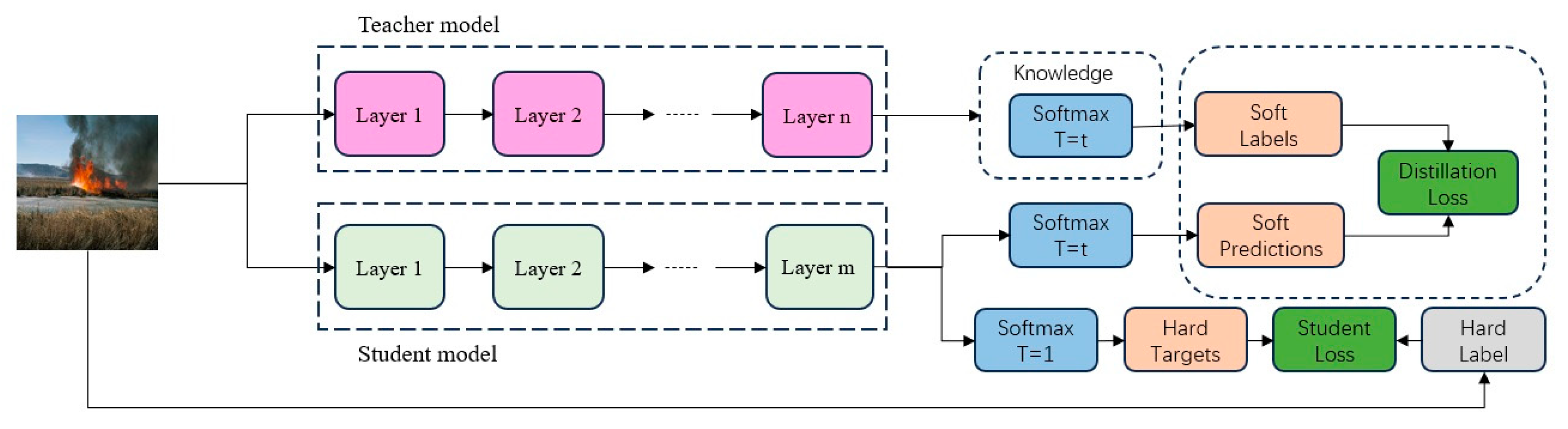
3.2. Knowledge Distillation Experimental Results

To ensure the accuracy of LightFireNet, the teacher model was chosen to supervise the training of its fire recognition model. The baseline models were selected to cover diverse architectures (deep networks for high-accuracy and lightweight networks for edge compatibility) and their proven effectiveness in image classification tasks. Experiments were conducted to compare the performance of various classical networks (including GoogLeNet [32], ResNet [33], MobileNet, SqueezeNet, ShuffleNet, EfficientNet [34], and InceptionV3 [35]) on the selected fire dataset, where GoogLeNet and ResNet are deep CNNs commonly used for complex classification tasks, while SqueezeNet, ShuffleNet, MobileNet, and EfficientNet are lightweight networks commonly used for mobile devices.

Table 3. Comparison of the effect of each network model on the self-built dataset.

Model	Model Size (MB)	Params (M)	FLOPs (M)	Accuracy	Precision	Recall	F1 Score
GoogLeNet [31]	21.37	5.60	275.04	98.42%	98.44%	98.42%	98.76%
ResNet-50 [32]	89.70	23.51	750.76	98.89%	98.91%	98.88%	98.89%
SqueezeNet	2.76	0.72	43.13	98.30%	98.32%	98.37%	98.34%
ShuffleNet	4.79	1.26	26.45	98.25%	97.74%	98.82%	98.28%
MobileNet-v2	8.50	2.29	55.05	98.77%	98.54%	98.98%	98.76%
EfficientNet [33]	15.30	4.01	71.20	98.25%	98.28%	98.16%	98.21%
InceptionV3 [34]	95.20	23.8	587	98.78%	98.82%	98.77%	98.78%
LightFireNet	0.09	0.024	9.11	95.91%	96.03%	95.84%	95.91%
Distilled	0.09	0.024	9.11	97.60%	97.67%	97.55%	97.60%

shows the performance of various network models on the fire dataset.

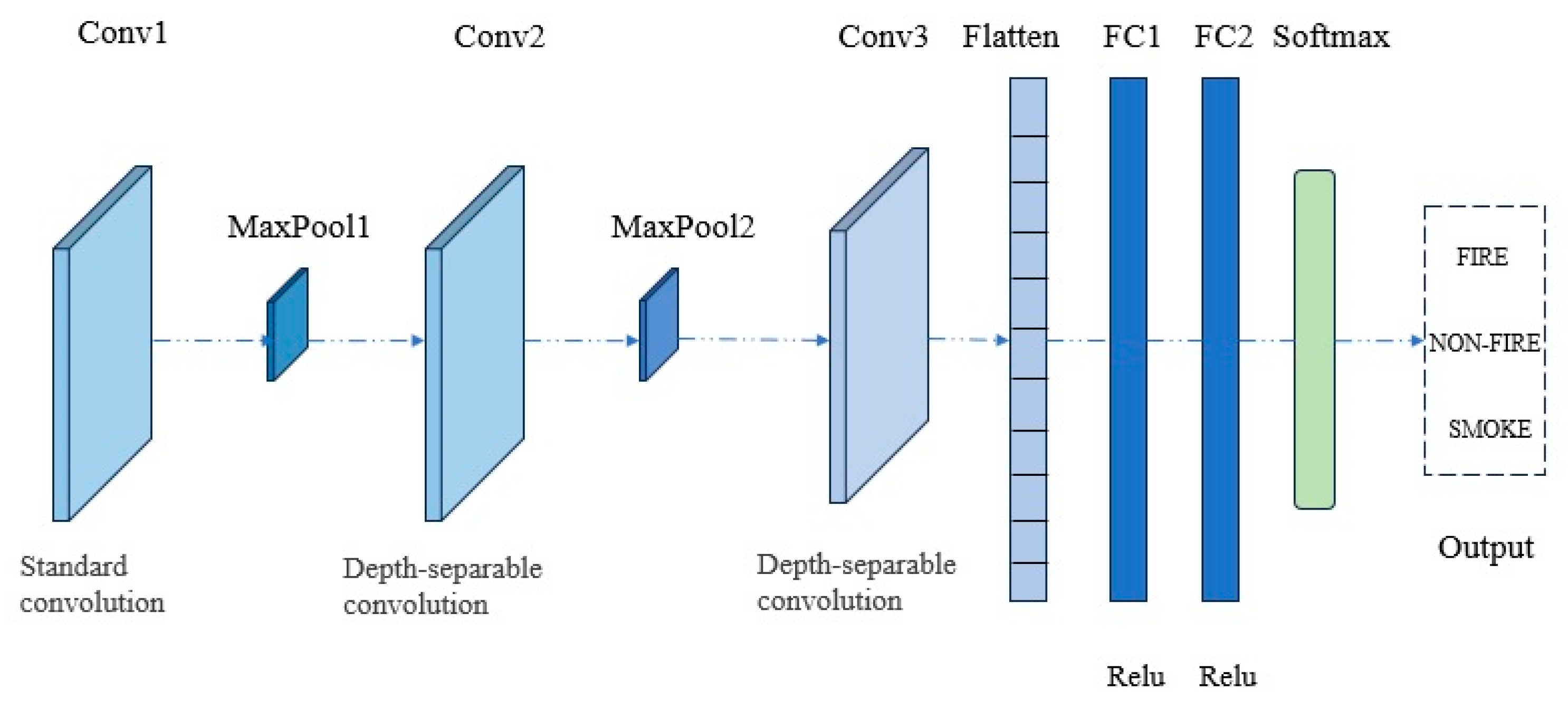
It can be seen from Table 3 that ResNet-50 has the best recognition effect, with an F1 score of 98.89%, followed by MobileNet-V2 and GoogLeNet, with F1 scores of 97.76%. Therefore, ResNet-50 was selected as the teacher network supervision for LightFireNet training. The accuracy of LightFireNet after the final knowledge distillation was 97.60%, and the F1 score was 97.60%. The recognition effect was improved compared with that before the knowledge distillation. It is worth noting that in our dataset, the recognition effect of MobileNet-V2 as a lightweight network is almost the same as that of GoogLeNet, a deep CNN, but the amount of parameters and calculations is much smaller than that of GoogLeNet. This is also the reason why LightFireNet adopts the same convolution method (depth-separable convolution) as MobileNet-V2 in its convolution layer design. After knowledge distillation, the parameter quantity of LightFireNet is only 1‰ of ResNet-50, and the calculation quantity is only 1.2% of ResNet50.

3.3. Forest Fire Recognition Effect of LightFireNet

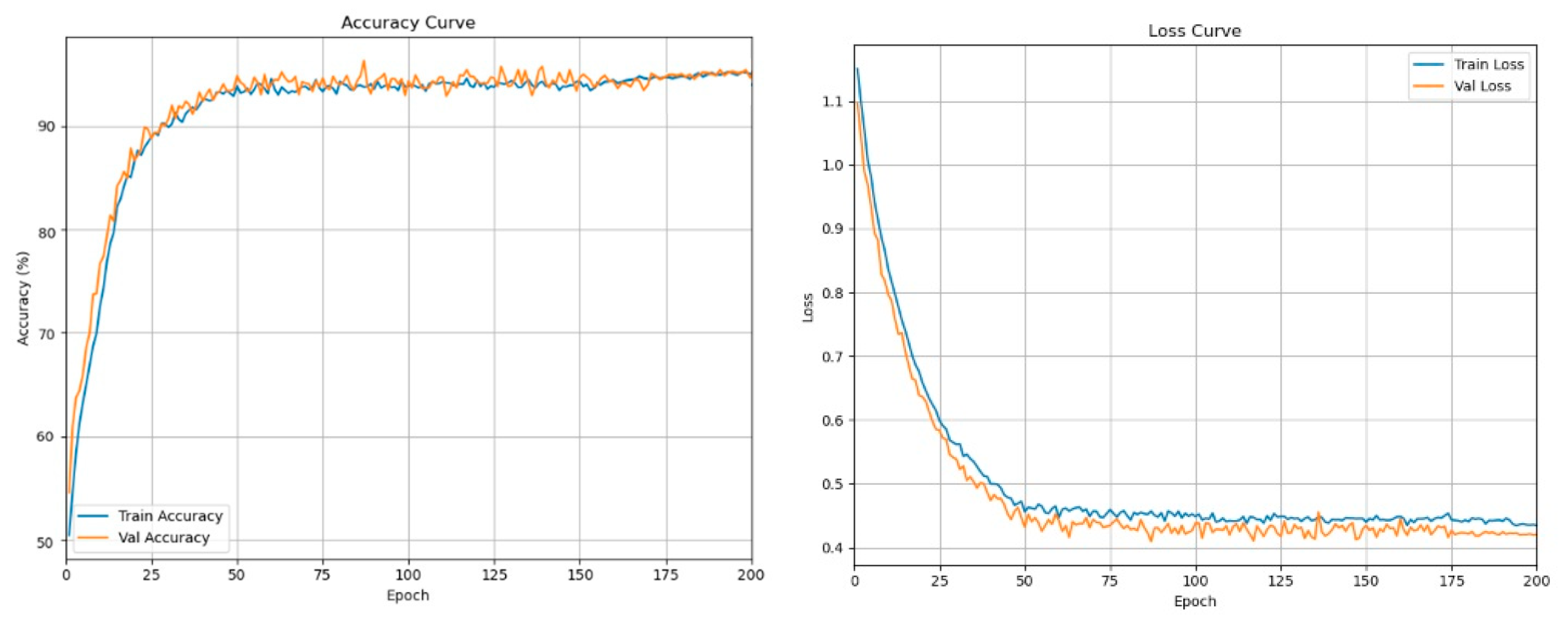
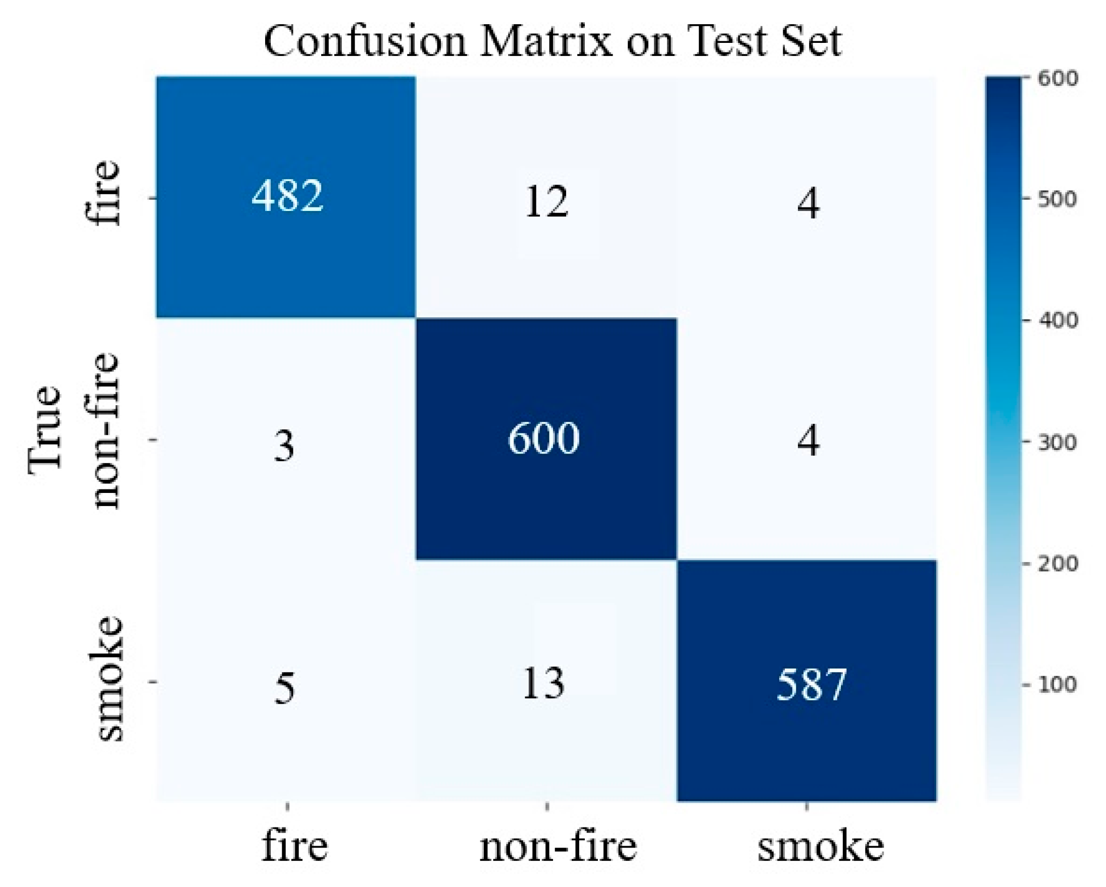
Figure 14 illustrates the training and validation curves, where both accuracy curves converge closely and loss curves decline steadily without divergence, indicating no overfitting. The recognition effect of LightFireNet on the test set is shown in Figure 15. It can be seen from the confusion matrix that the classification performance of the LightFireNet model on the test set is excellent. The model shows high accuracy in distinguishing fire, non-fire, and smoke, and can effectively realize the function of fire monitoring in a complex outdoor environment.

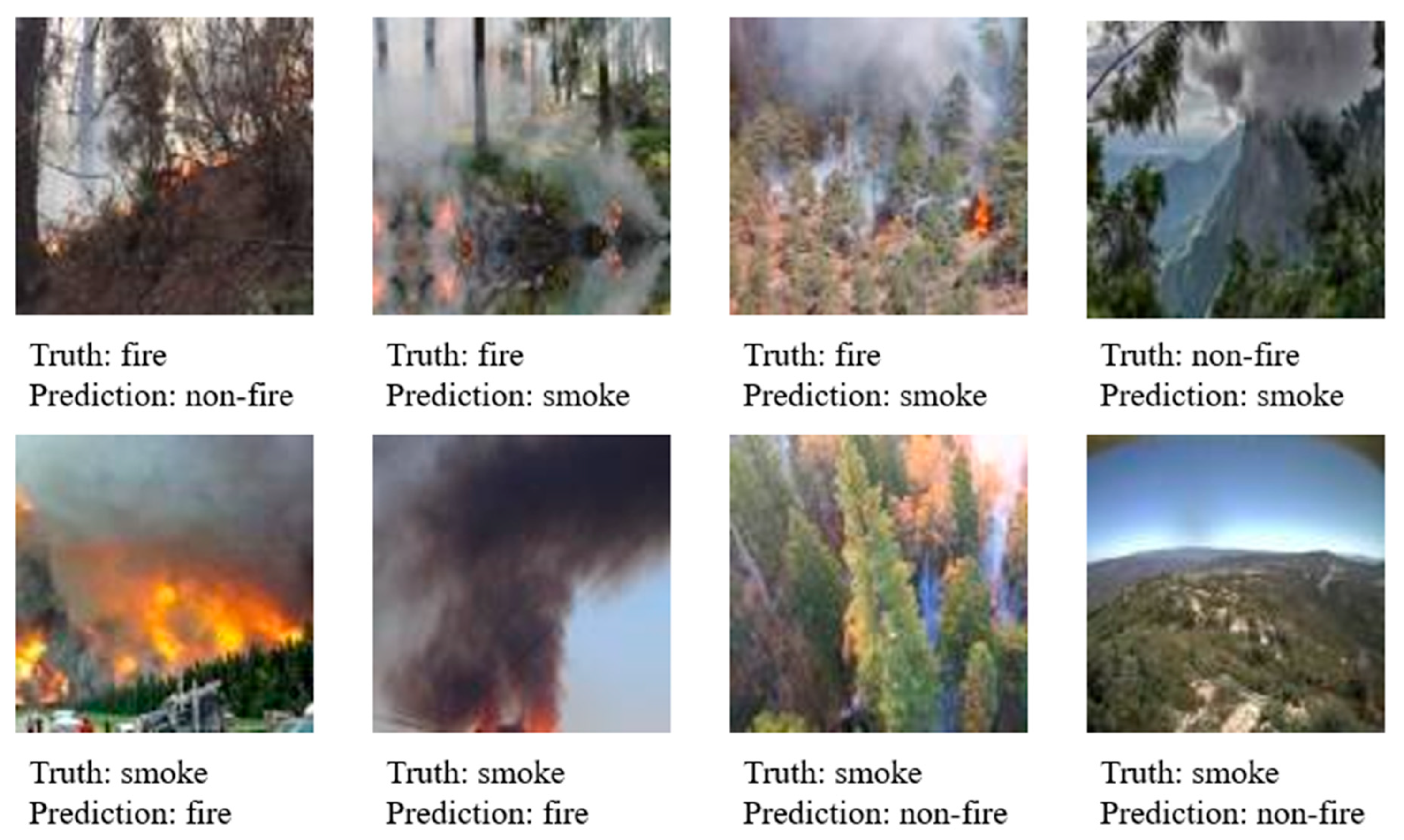
All recognition results and error analyses presented in this section are based on the 3 × 96 × 96 input size determined through our spatial resolution experiments in Section 3.4. This resolution was selected as the optimal balance between recognition accuracy and hardware deployment constraints, as detailed in Section 3.4 and Section 3.5. Figure 16 shows an example of the wrong image of the LightFireNet model for the classification of outdoor forest fire smoke. The first three “fire” pictures are predicted to be “non-fire” or “smoke”, which may be because the flame is partially obscured by smoke or the flame intensity is not enough to enable the model to extract significant features. The most obvious feature is that the proportion of the flame area in the picture is very small, while the proportion of the smoke area is very large, which causes the model to learn more about the characteristics of smoke. The same situation occurs in the “smoke” picture. Some scenes with thick smoke are wrongly classified as “fire”. It may be that the texture of smoke in the image is similar to that of fire, which leads to model confusion. In addition, the fourth “non-fire” scene was mistakenly predicted as a “smoke” category, which may be because the background in these images, such as remote haze, clouds, etc., is relatively similar to the smoke characteristics, leading to the inability of the model to distinguish correctly. From the misclassified examples in Figure 16, it is evident that the model occasionally struggles with highly ambiguous scenarios, such as smoke-obscured flames or scenes where smoke resembles clouds or haze. These cases are inherently challenging even for human observers, as the visual features of fire and smoke often overlap in complex environments. Despite these edge cases, LightFireNet achieves an accuracy of 97.60%, demonstrating robust performance in distinguishing fire, smoke, and non-fire scenes—a significant improvement over traditional binary classification approaches. This high accuracy, combined with the model’s lightweight design, validates its suitability for real-world forest fire monitoring.

3.4. Impact of Input Image Size on Model

In order to determine the impact of different input sizes on the recognition effect of LightFireNet, we conducted a comparative experiment with different input sizes. The experimental results are shown in

Table 4. Influence of different input sizes on forest fire recognition in LightFireNet.

Input Size	Model Size (MB)	Params (M)	FLOPs (M)	Accuracy	Precision	Recall	F1 Score
3 × 224 × 224	4.49	1.17	52.22	98.13%	98.16%	98.12%	98.13%
3 × 128 × 128	0.53	0.14	16.49	98.25%	98.21%	98.24%	98.23%
3 × 96 × 96	0.09	0.024	9.11	97.60%	97.67%	97.55%	97.60%
3 × 48 × 48	0.09	0.024	2.92	95.91%	95.93%	95.87%	95.90%

. The experimental results show that when the input size is set to 3 × 48 × 48, the recognition effect of the network is the worst, and the accuracy is less than 96%. When the input size is set to 3 × 128 × 128, the recognition effect of the network is the best, with an accuracy rate of 98.25% and an F1 score of 98.23%. However, when the input size is further increased to 3 × 224 × 224, the recognition accuracy is not further improved but the model parameters and computational complexity are significantly increased, which is not conducive to the deployment of lightweight models on edge devices. We chose 3 × 96 × 96 as the final input size. The recognition accuracy, precision recall rate, and F1 score of this size are less than 0.7 percentage points lower than those of 3 × 128 × 128 but the parameter amount is only 17% of the latter, and the calculation amount is only 55% of the latter. The final selection of 3 × 96 × 96 as the input size is based on the comprehensive consideration of the accuracy of the model and the balance of computing resource consumption. This size meets the computing power limit of the FPGA platform while achieving a better fire recognition effect.

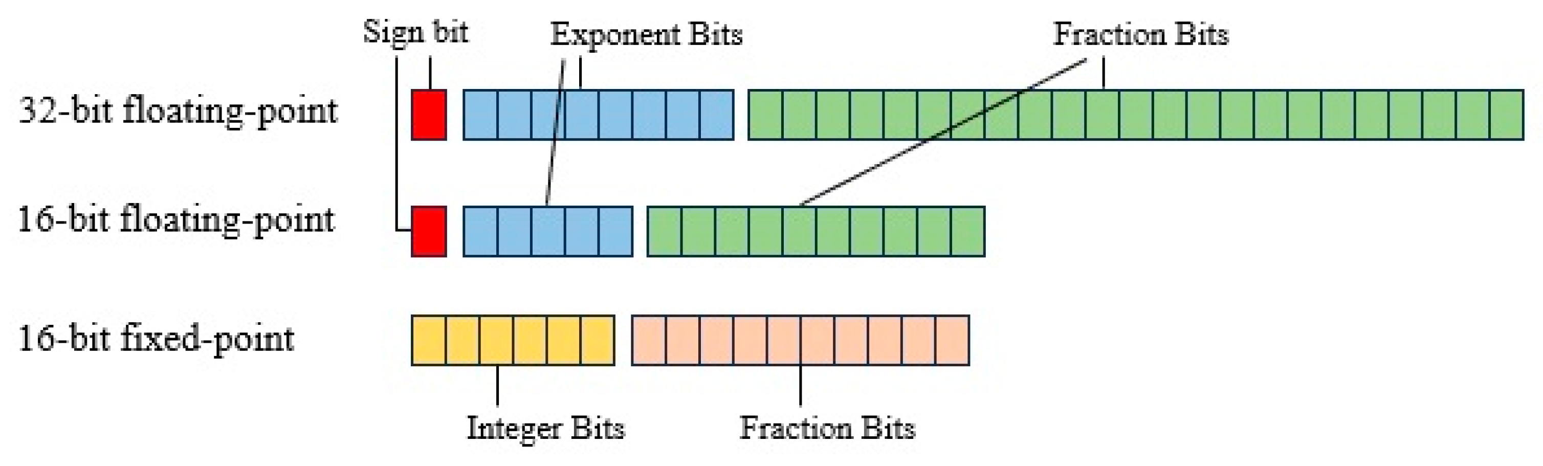
3.5. The Influence of Data Quantization on LightFireNet Hardware Circuit

In order to study the influence of different data types on the LightFireNet hardware circuit, we conducted experiments on three data types: single-precision floating point (32-bits), half-precision floating point (16-bits), and 16-bit fixed-point ap_fixed16. The experimental results show that when the data type is float32, the resource required by the optimized LightFireNet hardware circuit greatly exceeds the maximum resource provided by FPGA, so it cannot be successfully deployed in the specified FPGA. The half type and ap_fixed type can successfully accelerate FPGA implementation.

Table 5. Comparison of resource consumption and accuracy of different data types.

Type of Data	BRAM_18K	DSP	FF	LUT	Accuracy
float (32-bits)	\	\	\	\	97.60%
half (16-bits)	72	210	56,742	42,262	97.48%
ap_fixed (16-bits)	64	150	49,561	39,692	96.70%

shows the resource consumption of three data types of LightFireNet circuits. The difference between the half type and ap_fixed fixed-point digital type in DSP, FF, and LUT consumption is relatively small. Table 5 shows that in terms of model accuracy, the accuracy of the half type is 97.48%, and that of the ap_fixed type is 96.70%. Although the accuracy of the ap_fixed16 type is slightly lower than that of the half type, its resource consumption is lower. Considering the accuracy and resource consumption of the model, the ap_fixed16 type performs better in the FPGA.

3.6. Influence of Traditional Convolution and Depth-Separable Convolution on Complexity and Accuracy of Forest Fire Recognition Network

In order to optimize the computational complexity and model performance of LightFireNet, we compared the impact of Conventional Convolution and Separate Convolution on the recognition network. The results are shown in

Table 6. Comparison of different convolution methods.

Conv Method	Model Size (MB)	Params (M)	FLOPs (M)	Accuracy	Precision	Recall	F1 Score
Conventional Conv	0.64	0.17	21.21	97.95%	98.03%	97.92%	97.96%
Separable Conv	0.024	0.09	9.11	97.60%	97.67%	97.55%	97.60%

. The experimental results showed that the use of depth-separable convolution significantly reduces the amount of parameters and computation of the model while maintaining a high recognition accuracy. Among them, the size of the LightFireNet model implemented by Conventional Revolution is 0.64 MB, the number of parameters is 0.17 M, and the calculation amount is 21.21 M times. However, the size, parameter amount, and calculation amount of the LightFireNet model of Separate Revolution are far smaller than the former, which are 0.024 M, 0.09 M, and 9.11 M times, respectively. In terms of the recognition effect, the accuracy rate of depth-separable convolution is only 0.35 percentage points lower than that of traditional convolution, and the F1 score is only 0.36 percentage points lower than that of traditional convolution. Although the recognition effect has slightly declined, the decline is small and has a limited impact on the performance in practical applications.

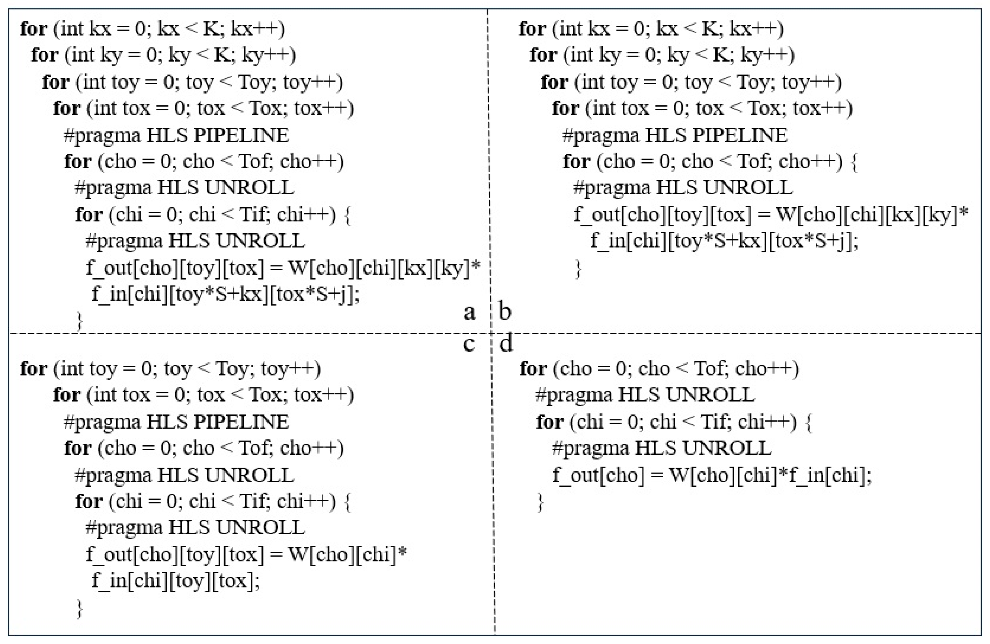
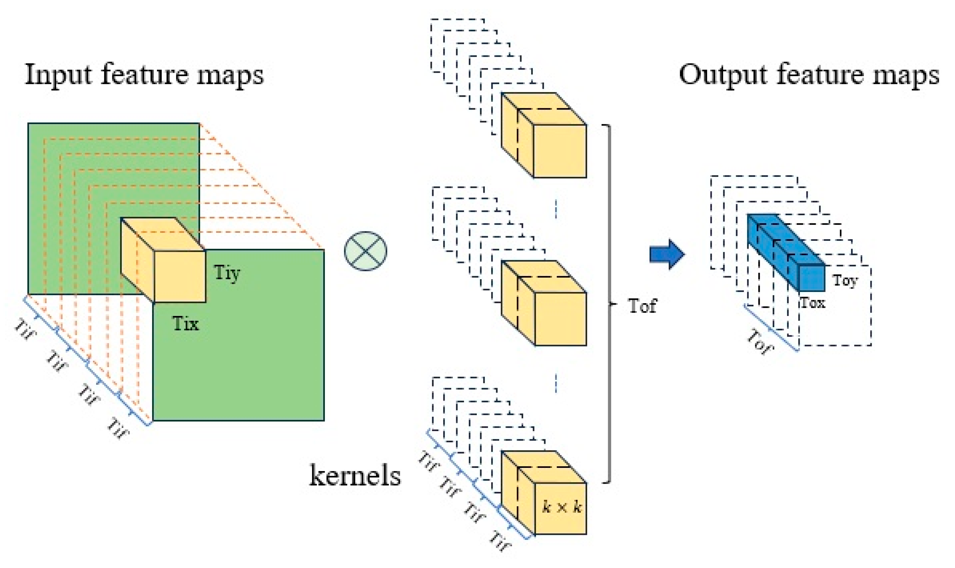
3.7. Influence of Loop Tiling Processing on LightFireNet Convolution Layer Circuits

Table 7. Latency and resource consumption of convolution before and after loop tiling.

Method	Latency (Mcycles)	BRAM_18K	DSP	FF	LUT
Normal	5.55	26	12	7557	7086
Loop Tiling	0.33	62	51	16,549	22,506

shows the impact of loop tiling on LightFireNet convolution layer circuits. Taking depthwise separable convolution as an example, when loop tiling is not used, the hardware resources consumed by convolution layer circuits include BRAM_18K: 26, DSP: 12, FF: 7557, and LUT: 7086. At this time, the delay of the convolution layer circuit is 5.55 Mcycles. When the loop tiling strategy is adopted, the hardware resources consumed by the convolution layer circuit increase significantly, which include BRAM_18K: 62, DSP: 51, FF: 16,549, and LUT: 22,506, in which the DSP usage of the latter is about four times that of the former, but at this time, the delay of the convolutional layer circuit is 0.33 Mcycles, which is 94.1% lower than that of the circuit without loop tiling. The loop tiling strategy makes full use of the limited resources of FPGA; cooperates with cyclic switching, the ping-pong buffer, and other technologies to exchange resources for time; greatly reduces the delay of convolution circuit; and speeds up the recognition process of forest fires.

3.8. Comparison of Forest Fire Recognition Effect Between FPGA and Other Devices (CPU, GPU, Raspberry Pie)

In this study, the processing effects of different computing platforms on forest fire recognition tasks were compared and analyzed. By comparing FPGA with a traditional central processing unit (CPU), graphics processing unit (GPU), and embedded system (such as raspberry pie), its performance in forest fire recognition was evaluated. The specific results are shown in

Table 8. Different devices realize the effect of forest fire recognition in LightFireNet.

Equipment	Accuracy	Speed (ms)	Power (w)	Price (RMB)
FPGA	96.70%	64	2.23	850
CPU	97.60%	1	35.8	3647
GPU+CPU	97.60%	0.3	28.5	7600
Raspberry Pi	97.60%	230	4.2	300
Android	97.60%	10	4.86	4188

Note: FPGA is ZYNQ Z7-Lite 7020 development board. CPU is Intel (R) Core (TM) i7-12700H 2.30 GHz; GPU is NVIDIA GeForce RTX 3050. Raspberry pie is the third-generation B type; soc is Broadcom BCM2837; Android is Huawei P40.

. The CPU is a laptop computer and the GPU is mounted on the CPU, forming a “GPU+CPU” graphic workstation. See the table notes for the specific models of each device.

First of all, the accuracy rate of FPGA is 96.70%, and that of other platforms is 97.60. This is because the network implemented by all devices is LightFireNet, while FPGA uses ap_fixed16-type data, and devices other than FPGA use float-type data. However, in other performance indicators, FPGA shows obvious advantages. In terms of processing speed, the recognition delay of FPGA is only 64 ms. Compared with 1 ms of CPU, 0.3 ms of GPU+CPU, 230 ms of Raspberry Pie, and 10 ms of Android, the speed performance of FPGA is at a medium level. However, in terms of power consumption, the energy efficiency performance of FPGA is excellent, and the power consumption is only 2.23 W. Compared with 35.8 W of CPU and 28.5 W of GPU+CPU, the low power consumption characteristics of FPGA make it have obvious application advantages in edge devices. Raspberry pie and Android are also competitive in terms of power consumption, which are 4.2 W and 4.86 W, respectively. Raspberry pie reasoning speed is significantly slower than FPGA, and Android device reasoning speed is faster than FPGA. The power consumption data are the instantaneous power during forest fire recognition, including GPU+CPU. The power of raspberry pie and Android is measured by HWiNFO software (Version 8.16-5600), and the power consumption of FPGA edge devices is directly measured by a power meter. In addition, in terms of price, FPGA and raspberry pie are more affordable than CPU, GPU+CPU, Android, and other high-performance computing platforms. FPGA is only CNY 850, while raspberry pie costs only CNY 300. The accuracy rate of FPGA in forest fire recognition is equivalent to that of CPU, GPU, and Android but it has the lowest power consumption, a smaller size, and stronger portability and mobility. Compared with raspberry pie, FPGA has similar portability and a slightly higher price but it has more advantages in power consumption and disease recognition speed. Overall, FPGA is superior to other devices in speed, accuracy, power consumption, portability, and price and is suitable for real-time forest fire recognition as an edge device in complex field environments.

3.9. Performance Testing Under Real Fire Video Conditions

To validate the effectiveness of the proposed FPGA-accelerated LightFireNet model in real-world scenarios, we conducted experiments using three real fire videos collected from online sources, which documented actual forest fire incidents and normal forest scenes. These raw videos were categorized and edited into three 30 s clips (30 fps) representing fire, non-fire, and smoke scenarios, respectively. Each processed video contains 900 frames in total. Due to the recognition speed of the FPGA device (64 ms per frame), the system processes every other frame to ensure real-time performance. Thus, out of 900 frames, 450 frames were actually recognized, achieving a practical recognition rate of 15 fps (450 frames/30 s). This demonstrates that the system can meet the real-time monitoring requirements for forest fires.

The experimental results are shown in

Table 9. Recognition performance on real fire videos.

Video	Total Frames	Recognized Frames	Correctly Recognized Frames	Accuracy
Video 1	900	450	443	98.44%
Video 2	900	450	445	98.89%
Video 3	900	450	435	96.67

. The accuracy of the system was calculated based on the correctly recognized frames. The results indicate that the proposed method maintains high accuracy even under real fire conditions, further validating its practical applicability.

The results demonstrate that the FPGA-accelerated LightFireNet model achieves an average accuracy of 98.00% across the three video categories, with fire recognition at 98.44%, non-fire at 98.89%, and smoke at 96.67%. These values are consistent with the performance on the test dataset (Section 3.3), confirming the robustness of the system in real-world scenarios. The high recognition accuracy for fire and non-fire categories can be attributed to two factors: (1) the inherent strong performance of the LightFireNet model as demonstrated in Section 3.3 and (2) the relatively stable scenes in these test videos with limited background variations. Notably, most misclassifications occurred in Video 3 (smoke category), where scenes containing both smoke and fire were frequently identified as “fire”—a pattern consistent with the error cases analyzed in Section 3.3 (Figure 16). These results validate the practical effectiveness of the FPGA-based forest fire recognition system while highlighting its tendency to prioritize fire detection in ambiguous smoke-fire scenarios, which aligns with the safety-critical nature of fire monitoring applications.

4. Discussion

The experimental results demonstrate that the proposed LightFireNet framework achieves an accuracy of 96.70% in the FPGA, with a processing speed of 64 ms per frame and a power consumption of only 2.23 W. These metrics highlight the effectiveness of the lightweight CNN design and FPGA acceleration in balancing computational efficiency and recognition performance. The success of this approach stems from several key innovations, including depthwise separable convolution, knowledge distillation, and hardware-aware optimizations such as loop tiling and data quantization. By reducing the model parameters to just 24 K and computations to 9.11 M, LightFireNet proves suitable for deployment in resource-constrained edge devices, offering a practical alternative to cloud-based or high-power GPU solutions.

The FPGA-accelerated LightFireNet framework presents significant practical value for forest science and management, particularly in the context of early fire detection and ecological monitoring. Its lightweight and low-power design enables flexible deployment across diverse environments, including forest watchtowers, tree canopies, and high-rise buildings. Due to its low cost, the system can be densely deployed to achieve large-scale, real-time monitoring of forest areas, addressing the limitations of traditional manual patrols and observation posts. Unlike cloud-based solutions that require high-bandwidth data transmission, this edge-computing approach minimizes the reliance on network connectivity—a critical advantage in remote forest areas with poor communication infrastructure. By processing data locally on FPGA devices, only the recognition results (e.g., fire alerts) need to be transmitted to central servers, significantly reducing latency and energy consumption while ensuring timely fire detection.

While IoT-based systems are valuable for large-scale environmental monitoring, they often face challenges such as high data transmission delays and dependency on stable network conditions. The proposed FPGA-accelerated solution complements IoT frameworks by offloading computationally intensive tasks to edge devices, thereby alleviating the storage and computing burdens typically associated with centralized systems. This hybrid approach enhances the scalability and responsiveness of forest fire monitoring systems, making them more adaptable to dynamic field conditions.

The fixed architecture of LightFireNet allows for easy updates by simply replacing the parameters stored on the SD card, without requiring hardware modifications. This feature ensures long-term adaptability to evolving monitoring needs, such as integrating additional sensors (e.g., thermal or infrared cameras) to improve detection robustness under varying environmental conditions. Future work could explore automated parameter updates and edge–cloud collaboration to further optimize performance.

Despite its advantages, the current implementation has limitations, such as a slight accuracy drop due to fixed-point quantization, which may affect performance in edge cases like heavily obscured fires. Future research could investigate hybrid quantization strategies or multi-modal data fusion to enhance detection accuracy. Additionally, real-world field testing is needed to validate the system’s reliability under extreme weather conditions or long-term operational stress.

5. Conclusions

This study bridges the gap between computer science innovations and practical forest management needs by providing a cost-effective, energy-efficient solution for early fire detection. The methodologies developed here can also be extended to other ecological applications, such as biodiversity monitoring or tree health assessment, contributing to the broader goals of sustainable forest management and conservation. By combining edge computing with lightweight AI, this work lays the foundation for scalable, intelligent monitoring systems tailored to the challenges of modern forestry.

Beyond its technical contributions, this work addresses critical challenges in forest management by providing a low-cost, energy-efficient solution for early fire detection, particularly in areas with unreliable network connectivity. While IoT systems play a valuable role in large-scale monitoring, our approach prioritizes edge computing to ensure real-time responsiveness, offering a complementary solution that can operate independently or within broader IoT networks. The methodologies developed here, including model compression and hardware acceleration techniques, are not limited to fire detection; they can be adapted to other ecological applications such as biodiversity monitoring or tree health assessment, extending their impact across environmental research.

Looking ahead, future work will explore hybrid architectures combining FPGA efficiency with IoT scalability, as well as multi-modal sensor integration, to enhance detection robustness. We aim to foster collaboration between computer scientists and forest researchers, ensuring that these innovations translate into tangible benefits for wildfire prevention and ecosystem conservation. This study underscores the potential of lightweight, edge-optimized AI to transform forest monitoring, offering both theoretical insights and practical tools for sustainable land management.

References

1. Qian, J.; Lin, H. A Forest Fire Identification System Based on Weighted Fusion Algorithm. Forests 2022, 13, 1301. [Google Scholar] [CrossRef]
2. Barmpoutis, P.; Papaioannou, P.; Dimitropoulos, K.; Grammalidis, N. A Review on Early Forest Fire Detection Systems Using Optical Remote Sensing. Sensors 2020, 20, 6442. [Google Scholar] [CrossRef] [PubMed]
3. Wu, S.; Sheng, B.; Fu, G.; Zhang, D.; Jian, Y. Multiscale fire image detection method based on CNN and Transformer. Multimed. Tools Appl. 2024, 83, 49787–49811. [Google Scholar] [CrossRef]
4. Celik, T.; Ozkaramanlt, H.; Demirel, H. Fire Pixel Classification using Fuzzy Logic and Statistical Color Model. In Proceedings of the 2007 IEEE International Conference on Acoustics, Speech and Signal Processing—ICASSP’07, Honolulu, HI, USA, 15–20 April 2007; pp. I-1205–I-1208. [Google Scholar]
5. Ha, C.; Hwang, U.; Jeon, G.; Cho, J.; Jeong, J. Vision-Based Fire Detection Algorithm Using Optical Flow. In Proceedings of the 2012 Sixth International Conference on Complex, Intelligent, and Software Intensive Systems, Palermo, Italy, 4–6 July 2012; pp. 526–530. [Google Scholar]
6. Zhang, Z.; Shen, T.; Zou, J. An Improved Probabilistic Approach for Fire Detection in Videos. Fire Technol. 2014, 50, 745–752. [Google Scholar] [CrossRef]
7. Marbach, G.; Loepfe, M.; Brupbacher, T. An image processing technique for fire detection in video images. Fire Saf. J. 2006, 41, 285–289. [Google Scholar] [CrossRef]
8. Bai, X.; Wang, Z. Research on Forest Fire Detection Technology Based on Deep Learning. In Proceedings of the 2021 International Conference on Computer Network, Electronic and Automation (ICCNEA), Xi’an, China, 24–26 September 2021; pp. 85–90. [Google Scholar]
9. Sathishkumar, V.E.; Cho, J.; Subramanian, M.; Naren, O.S. Forest fire and smoke detection using deep learning-based learning without forgetting. Fire Ecol. 2023, 19, 9. [Google Scholar] [CrossRef]
10. Khan, S.; Khan, A. Deep Learning Based Forest Fire Classification and Detection in Smart Cities. Symmetry 2022, 14, 2155. [Google Scholar] [CrossRef]
11. Peng, Y.; Wang, Y. Real-time forest smoke detection using hand-designed features and deep learning. Comput. Electron. Agric. 2019, 167, 105029. [Google Scholar] [CrossRef]
12. Zhang, J.; Zhu, H.; Wang, P.; Ling, X. ATT Squeeze U-Net: A Lightweight Network for Forest Fire Detection and Recognition. Inst. Electr. Electron. Eng. Access 2021, 9, 10858–10870. [Google Scholar] [CrossRef]
13. Chen, Y.; Zhang, Y.; Xin, J.; Wang, G.; Mu, L.; Yi, Y.; Liu, H.; Liu, D. UAV Image-based Forest Fire Detection Approach Using Convolutional Neural Network. In Proceedings of the 2019 14th IEEE Conference on Industrial Electronics and Applications (ICIEA), Xi’an, China, 19–21 June 2019; pp. 2118–2123. [Google Scholar]
14. Liu, Y.; Sun, R.; Zhang, T.; Zhang, X.; Li, L.; Shi, G. Fast Fire Identification Soft-Core Package Design Based on FPGA. In Proceedings of the 2020 International Conferences on Internet of Things (iThings) and IEEE Green Computing and Communications (GreenCom) and IEEE Cyber, Physical and Social Computing (CPSCom) and IEEE Smart Data (SmartData) and IEEE Congress on Cybermatics (Cybermatics), Rhodes Island, Greece, 2–6 November 2020; pp. 642–647. [Google Scholar]
15. Grari, M.; Yandouzi, M.; Idrissi, I.; Boukabous, M.; Moussaoui, O.; Azizi, M.; Moussaoui, M. Using IoT and Ml for Forest Fire Detection, Monitoring, and Prediction: A Literature Review. J. Theor. Appl. Inf. Technol. 2022, 100, 5445–5461. [Google Scholar] [CrossRef]
16. Cao, K.; Liu, Y.; Meng, G.; Sun, Q. An Overview on Edge Computing Research. Inst. Electr. Electron. Eng. Access 2020, 8, 85714–85728. [Google Scholar] [CrossRef]
17. Hussain, T.; Dai, H.; Gueaieb, W.; Sicklinger, M.; De Masi, G. UAV-based Multi-scale Features Fusion Attention for Fire Detection in Smart City Ecosystems. In Proceedings of the 2022 IEEE International Smart Cities Conference (ISC2), Pafos, Cyprus, 26–29 September 2022; pp. 1–4. [Google Scholar]
18. Howard, A.G.; Zhu, M.; Chen, B.; Kalenichenko, D.; Wang, W.; Weyand, T.; Andreetto, M.; Adam, H. MobileNets: Efficient Convolutional Neural Networks for Mobile Vision Applications. arXiv 2017, arXiv:1704.04861. [Google Scholar] [CrossRef]
19. Iandola, F.N.; Han, S.; Moskewicz, M.W.; Ashraf, K.; Dally, W.J.; Keutzer, K. SqueezeNet: AlexNet-level accuracy with 50x fewer parameters and <0.5 MB model size. arXiv 2016, arXiv:1602.07360. [Google Scholar] [CrossRef]
20. Zhang, X.; Zhou, X.; Lin, M.; Sun, J. ShuffleNet: An Extremely Efficient Convolutional Neural Network for Mobile Devices. In Proceedings of the 2018 IEEE/CVF Conference on Computer Vision and Pattern Recognition, Salt Lake City, UT, USA, 18–23 June 2018; pp. 6848–6856. [Google Scholar]
21. Almeida, J.S.; Huang, C.; Nogueira, F.G.; Bhatia, S.; de Albuquerque, V.H.C. EdgeFireSmoke: A Novel Lightweight CNN Model for Real-Time Video Fire–Smoke Detection. IEEE Trans. Ind. Inform. 2022, 18, 7889–7898. [Google Scholar] [CrossRef]
22. Wang, S.; Zhao, J.; Ta, N.; Zhao, X.; Xiao, M.; Wei, H. A real-time deep learning forest fire monitoring algorithm based on an improved Pruned + KD model. J. Real-Time Image Process. 2021, 18, 2319–2329. [Google Scholar] [CrossRef]
23. Qiu, J.; Wang, J.; Yao, S.; Guo, K.; Li, B.; Zhou, E.; Yu, J.; Tang, T.; Xu, N.; Song, S.; et al. Going Deeper with Embedded FPGA Platform for Convolutional Neural Network. In Proceedings of the 2016 ACM/SIGDA International Symposium on Field-Programmable Gate Arrays, Monterey, CA, USA, 21–23 February 2016; ACM: Monterey, CA, USA, 2016; pp. 26–35. [Google Scholar]
24. Shawahna, A.; Sait, S.M.; El-Maleh, A. FPGA-Based Accelerators of Deep Learning Networks for Learning and Classification: A Review. Inst. Electr. Electron. Eng. Access 2019, 7, 7823–7859. [Google Scholar] [CrossRef]
25. Cornu, A.; Derrien, S.; Lavenier, D. HLS Tools for FPGA: Faster Development with Better Performance. In Reconfigurable Computing: Architectures, Tools and Applications; Koch, A., Krishnamurthy, R., McAllister, J., Woods, R., El-Ghazawi, T., Eds.; Lecture Notes in Computer Science; Springer: Berlin/Heidelberg, Germany, 2011; Volume 6578, pp. 67–78. ISBN 978-3-642-19474-0. [Google Scholar]
26. Hinton, G.; Vinyals, O.; Dean, J. Distilling the Knowledge in a Neural Network. arXiv 2015, arXiv:1503.02531. [Google Scholar]
27. Li, Y.; Song, B.; Kang, X.; Du, X.; Guizani, M. Vehicle-Type Detection Based on Compressed Sensing and Deep Learning in Vehicular Networks. Sensors 2018, 18, 4500. [Google Scholar] [CrossRef]
28. Mittal, S. A survey of FPGA-based accelerators for convolutional neural networks. Neural. Comput. Applic. 2020, 32, 1109–1139. [Google Scholar] [CrossRef]
29. Krizhevsky, A.; Sutskever, I.; Hinton, G.E. ImageNet classification with deep convolutional neural networks. Commun. ACM 2017, 60, 84–90. [Google Scholar] [CrossRef]
30. Bacon, D.F.; Graham, S.L.; Sharp, O.J. Compiler transformations for high-performance computing. ACM Comput. Surv. 1994, 22, 345–420. [Google Scholar] [CrossRef]
31. Zhang, C.; Li, P.; Sun, G.; Guan, Y.; Xiao, B.; Cong, J. Optimizing FPGA-based Accelerator Design for Deep Convolutional Neural Networks. In Proceedings of the 2015 ACM/SIGDA International Symposium on Field-Programmable Gate Arrays, Monterey, CA, USA, 22–24 February 2015; pp. 161–170. [Google Scholar]
32. Szegedy, C.; Liu, W.; Jia, Y.; Sermanet, P.; Reed, S.; Anguelov, D.; Erhan, D.; Vanhoucke, V.; Rabinovich, A. Going Deeper with Convolutions. In Proceedings of the 2015 IEEE Conference on Computer Vision and Pattern Recognition (CVPR), Boston, MA, USA, 7–12 June 2015; pp. 1–9. [Google Scholar]
33. He, K.; Zhang, X.; Ren, S.; Sun, J. Deep Residual Learning for Image Recognition. In Proceedings of the 2016 IEEE Conference on Computer Vision and Pattern Recognition (CVPR), Las Vegas, NV, USA, 27–30 June 2016; pp. 770–778. [Google Scholar]
34. Tan, M.; Le, Q.V. EfficientNet: Rethinking Model Scaling for Convolutional Neural Networks. arXiv 2020, arXiv:1905.11946. [Google Scholar]
35. Szegedy, C.; Vanhoucke, V.; Ioffe, S.; Shlens, J.; Wojna, Z. Rethinking the Inception Architecture for Computer Vision. In Proceedings of the IEEE Conference on Computer Vision and Pattern Recognition, Las Vegas, NV, USA, 27–30 June 2016; pp. 2818–2826. [Google Scholar]
Figure 1. Structure diagram of ZYNQ Z7-Lite 7020 development board.
Forests 16 00698 g001
Figure 2. System Flow.
Forests 16 00698 g002
Figure 3. Some representative images of fire, no fire, and smoke in our dataset. (a) Fire images include small fires and large fires; (b) Non-fire images include fire clouds similar to fire, red leaf forests, and clouds similar to smoke; (c) Smoke images include small smoke and large smoke.
Forests 16 00698 g003
Figure 4. Forest fire smoke recognition model LightFireNet network structure.
Forests 16 00698 g004
Figure 5. Network layer pseudo-code. (a) Standard convolution; (b) Depth convolution, (c) Point-by-point convolution; (d) Full connection layer.
Forests 16 00698 g005
Figure 6. The circuit structure of forest fire recognition based on LightFireNet.
Forests 16 00698 g006
Figure 7. Traditional convolution and depth-separable convolution. (a) Traditional convolution; (b) depth-separable convolution.
Forests 16 00698 g007
Figure 8. Knowledge distillation diagram.
Forests 16 00698 g008
Figure 9. BN merge process. (a) Before BN merge operation; (b) after BN merge operation.
Forests 16 00698 g009
Figure 10. The schematic diagram of three types of data structures.
Forests 16 00698 g010
Figure 11. Loop tiling.
Forests 16 00698 g011
Figure 12. Ping-pong buffer timing chart.
Forests 16 00698 g012
Figure 13. Multi-channel data transmission.
Forests 16 00698 g013
Figure 14. Training and validation curves.
Forests 16 00698 g014
Figure 15. Confusion matrix.
Forests 16 00698 g015
Figure 16. Example of wrong pictures of forest fire classification.
Forests 16 00698 g016