Article

Growing Stock Volume Estimation in Forest Plantations Using Unmanned Aerial Vehicle Stereo Photogrammetry and Machine Learning Algorithms

by
Mei Li
1,
Zengyuan Li
2,
Qingwang Liu
2,* and
Erxue Chen
2
1
Carbon Neutrality Research Center, Shijiazhuang University, Shijiazhuang 050035, China
2
Research Institute of Forest Resources Information Technique, Chinese Academy of Forestry, Beijing 100091, China
*
Author to whom correspondence should be addressed.
Forests 2025, 16(4), 663; https://doi.org/10.3390/f16040663
Submission received: 12 March 2025 / Revised: 4 April 2025 / Accepted: 9 April 2025 / Published: 10 April 2025
(This article belongs to the Section Forest Inventory, Modeling and Remote Sensing)

Abstract

:
Currently, it is very important to accurately estimate growing stock volumes; it is crucial for quantitatively assessing forest growth and formulating forest management plans. It is convenient and quick to use the Structure from Motion (SfM) algorithm in computer vision to obtain 3D point cloud data from captured highly overlapped stereo photogrammetry images, while the optimal algorithm for estimating growing stock volume varies across different data sources and forest types. In this study, the performance of UAV stereo photogrammetry (USP) in estimating the growing stock volume (GSV) using three machine learning algorithms for a coniferous plantation in Northern China was explored, as well as the impact of point density on GSV estimation. The three machine learning algorithms used were random forest (RF), K-nearest neighbor (KNN), and support vector machine (SVM). The results showed that USP could accurately estimate the GSV with R2 = 0.76–0.81, RMSE = 30.11–35.46, and rRMSE = 14.34%–16.78%. Among the three machine learning algorithms, the SVM showed the best results, followed by RF. In addition, the influence of point density on the estimation accuracy for the USP dataset was minimal in terms of R2, RMSE, and rRMSE. Meanwhile, the estimation accuracies of the SVM became stable with a point density of 0.8 pts/m2 for the USP data. This study evidences that the low-density point cloud data derived from USP may be a good alternative for UAV Laser Scanning (ULS) to estimate the growing stock volume of coniferous plantations in Northern China.

1. Introduction

Forest plantations account for 7.3% of the world`s forest-covered areas and provide vital products and ecosystem services, such as fuel material and wood, in addition to contributing to soil and watershed conservation, climate change mitigation, and carbon sequestration [1]. Planted forests account for 36.45% of the forest-covered areas in China [2] and play an essential role in achieving carbon peak and neutrality goals. It is necessary to efficiently and accurately identify the parameters reflecting forest growth and the status of management interventions. The growing stock volume is a dominant parameter of the National Forest Inventory (NFI) worldwide and is a crucial indicator of carbon storage and productivity [3]. The accurate and up-to-date estimation of growing stock volume is very important for the quantitative evaluation of forest growth, as well as for forest management planning [4].
Traditionally, forest structural attributes are obtained by field investigations, which are costly, laborious, and limited to small areas [5]. Active remote sensing technology, such as Light Detection and Ranging (LiDAR), has attracted substantial attention from foresters all over the world. Laser pulses penetrate forest canopies, acquiring accurate three-dimensional (3D) point cloud data. This shows great potential in forest structural attribute estimation and mapping, especially when solving the saturation problems in optical sensor and SAR data [6,7]. Airborne LiDAR (also referred as airborne laser scanning, ALS) has been widely employed to model and estimate forest structural attributes [8,9,10] in many countries and can support forest inventories at the individual tree level [11,12] and the plot or stand level [13,14]. Highly overlapped images provide 3D structure information, which is attributed to the remarkable progress in stereo photogrammetry. The vertical distributions of the 3D point clouds from stereo photogrammetry and LiDAR are clearly different due to their acquisition principles. The 3D point clouds of stereo photogrammetry mainly represent the upper canopy. The substantial interest in 3D point clouds from stereo photogrammetry is mainly attributed to its relatively low acquisition cost compared with that of LiDAR [15].
Some studies have compared the performances of these two kinds of 3D point cloud in estimating forest structural attributes [16,17]. Vastaranta et al. [18] compared the abilities of airborne stereo photogrammetry (also referred to as digital aerial photogrammetry, DAP) and ALS to estimate forest structural attributes, including the mean diameter, the mean height, the basal area, and the aboveground biomass and volume for single-layered, even-aged stands using a random forest (RF) algorithm. Iqbal et al. [16] studied the estimated accuracy of growing stock volume using point cloud metrics from ALS and DAP at the plot level using an RF algorithm. Tompalski et al. [19] quantified the prediction accuracy of Lorey’s mean height, the mean diameter, the basal area, and the volume using common metrics from DAP and ALS data and spectral metrics from DAP at the plot level using an RF algorithm. Most previous comparisons between DAP and ALS using an area-based approach found that the ALS data showed a slightly better performance than the DAP data for forest structural attribute estimation [20,21]. However, 3D point clouds derived from airborne stereo photogrammetry or airborne laser scanning are too expensive for frequent use, inconvenient, and unprofessional.
UAV remote sensing has rapidly developed in recent years and has great potential for forest applications [22,23], especially stereo photogrammetry when acquired using a low-cost UAV platform and camera. Liu et al. [24] analyzed the capability of ULS to estimate growing stock volume at the plot and tree levels in Ginkgo plantations using RF, K-nearest neighbor (KNN), and partial least squares (PLS). The results showed that KNN had a relatively high prediction accuracy. Corte et al. [25] estimated the growing stock volume based on tree-level ULS metrics using RF, support vector machine (SVM), artificial neural network (ANN), and extreme gradient boosting (XGBoost) algorithms with the common metric of a point cloud for a Eucalyptus benthamii plantation. It was found that the SVM algorithm had the best performance with the lowest error rates. Zhang et al. [26] analyzed the canopy characteristic parameters of different tree species using multiple linear regression (MLR), SVM, and RF models. The results showed that the RF model was better than that of the SVR and MLR models. Teshome et al. [27] employed three non-linear machine learning (ML) algorithms including RF, SVM, and KNN to predict plant biomass. The results indicated that UAV imaging in combination with ML models could be effectively utilized for monitoring plant biomass, and KNN and SVM outperformed RF. However, these existing studies indicate that the best algorithm for different data and forest types is not always consistent. In addition, the performances of ULS and USP point clouds for growing stock volume estimation have not been thoroughly compared and analyzed by commonly used machine learning algorithms in a plantation forest.
Furthermore, the point clouds of ULS and USP generally have a high density, which is a great challenge in large-area data processing. The point cloud can be thinned based on the point density per unit, point horizontal spacing, or point vertical height distribution [24], and then used to estimate the forest parameters. The effect of randomly removing points using LiDAR on aboveground biomass (AGB) to achieve the desired density has been analyzed [28,29]. The estimation accuracy of AGB at the plot level was only slightly affected by the pulse density. However, the influences of the point density of 3D point cloud data derived from ULS and USP on growing stock volume estimated using common machine learning algorithms are still unclear.
This study aimed to analyze the specific differences and abilities of point cloud data derived from USP based on some widely used machine learning algorithms to estimate the area-based growing stock volume of a coniferous plantation in the mountainous area of Northern China, including its vertical distribution. RF, SVM, and KNN were used to estimate the growing stock volume; the total and first echoes of ULS estimation were used as the reference to evaluate the performance of the USP data. In addition, the effects of the point density of the USP data on the estimation accuracy of growing stock volume were identified by randomly thinning the point cloud to a certain density.

2. Materials and Methods
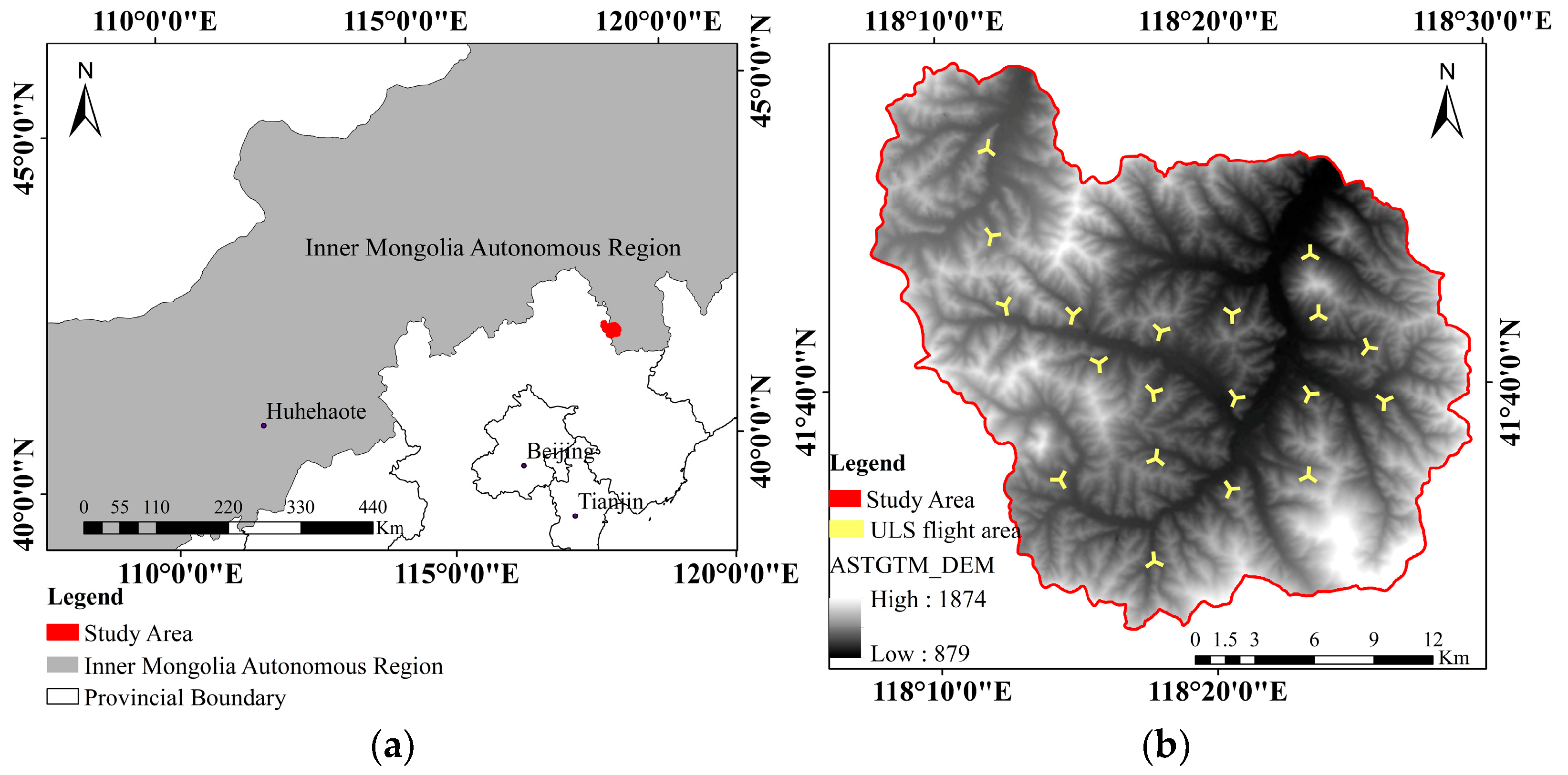
2.1. Study Site

The study site is located at the Wangyedian Forest Farm (118°09′–118°30′ E, 41°21′–41°39′ N) in Inner Mongolia Autonomous Province, China (Figure 1), in a mid-temperate, semi-arid, continental monsoon climate zone. The study area extends 24 km in the north–south direction and 21 km in the east–west direction, with a total area of approximately 500 km2. It is a typical plantation in this mountainous area with an altitude that varies from 800 m to 1890 m above sea level. The annual temperature ranges −31–36 °C, with a mean of about 4.2 °C. Annual precipitation totals about 400 mm–600 mm, and it mainly rains in July and August. The planted forest is mainly covered by Larix principis-rupprechtii and Pinus tabuliformis, with some naturally growing tree species. An actual photo of L. principis-rupprechtii plantations can be found in Figure 2.

2.2. Field Plot Data

A total of 71 square plots (25 m × 25 m) were established within the study area, and field work was conducted in September 2019. The four corners and center positions of each plot were geolocated using a differential GNSS receiver. In each plot, the living individual trees with a diameter at breast height (DBH, cm) ≥ 5 cm were selected as the sample trees; the species, DBH (cm), tree height (h, m), and crown width (m) at the perpendicular directions of east–west (EW) and north–south (NS) were recorded. The DBH of a tree was measured using a DBH tape. The tree height was measured with a laser rangefinder. Crown width (CW) was calculated as the average in the two directions. The volume of each tree was calculated using DBH and tree height based on the volume equations given in Table 1 [30]. Subsequently, the volume of each individual tree was accumulated and transformed into volume in m3 per hectare (V, m3/hm2) for each plot. The number of living individual trees within the 71 plots ranged from 28 to 254. The average DBH and the average height of the 71 plots varied from 7.7 cm to 31.2 cm and from 6.5 m to 20.5 m, respectively (Table 2).

2.3. UAV Laser Scanning (ULS) Data

The ULS data were acquired using a Riegl VUX-1 laser scanner (RIEGL Laser Measurement Systems GmbH, Horn, Austria) mounted on an eight-rotor UAV (RC6-2000) in September and October 2019 (see Table 3). The mean point density varied from 107 to 152 pts/m2 in the flight area. The flying heights varied from 933 m to 1322 m above ground level. The original point clouds were georeferenced using high-precision position and orientation data, and then projected to the coordinate system of the Universal Transverse Mercator Zone 50N/WGS-84. The vertical accuracy of the LiDAR data ranged from 0.19 m to 0.36 m.
The ULS point clouds were classified as ground, vegetation, etc. The ground points were used to generate a digital elevation model (DEM) using the triangular irregular networks algorithm. The height of the classified point clouds was normalized using the DEM derived from ULS.

2.4. UAV Stereo Photogrammetry (USP) Data

An easy-to-use and lightweight UAV with a visible camera (DJI Phantom 4 RTK, DJI, Nanshan, China) was used to capture the USP data in September 2019. The overlap was set to 80% and 70% in the longitudinal and lateral directions, respectively. A total of 14,000 images were acquired during 48 flights across 19 blocks on a sunny day. The designed flying height was approximately 190 m above ground level. Detailed parameters of the USP system are shown in Table 3.
The dense point clouds of USP were generated from image pairs using Agisoft Metashape professional (Version 1.6.2 build 10247). The processing mainly included image alignment, dense point cloud reconstruction, dense point cloud classification, and image orthorectification using Agisoft PhotoScan software (Version 1.6.2 build 10247). The image alignment used the original images with the key point limit of 40,000 and the tie point limit of 4000. The dense point cloud reconstruction used images downscaled by a factor of 4 (2 times each side) with the mild depth filtering mode to distinguish small details of trees. The point densities of the 19 blocks varied from 40 to 75 pts/m2. The dense point clouds were classified using a similar method as that for ULS data and were normalized using the DEM derived from ULS. The images were orthorectified with the mosaic blending mode at a pixel size of 0.01 m.

2.5. Feature Extraction

The features at the plot level mainly include height percentiles and height statistical and canopy density metrics (Table 4), which have been widely used to predict forest structural attributes [31]. The height percentiles and the height statistical metrics were calculated using the point clouds without points at a height of less than 2 m to eliminate the impact of shrubs, herbs, and the ground. The used height percentiles included h25, h50, h75, and h95. The height statistical metrics were the maximum (hmax), standard deviation (hsd), the mean (hmean), the variation coefficient (hcv), kurtosis (hkurt), and the interquartile range (hIQ) of the point clouds with a height ≥ 2 m. Additionally, the canopy relief ratio (CRR, represents canopy cover to some extent) and the percentage of points above the mean and mode height (CCmean and CCmod) were selected as the canopy density metrics, reflecting the vertical concentration of point clouds to some extent. The above-mentioned features were extracted from the first echoes of ULS and the dense point cloud of USP for growing stock volume estimation.

2.6. Growing Stock Volume Modeling and Evaluation

Three commonly used machine learning algorithms, namely RF, KNN, and SVM, were applied to develop models for predicting growing stock volume using the features from the ULS, USP, and field measurement data. These algorithms were run in the R environment with the ‘randomForest’ package for RF, the ‘caret’ package for KNN, and the ‘kernlab’ package for the SVM, respectively. A brief description of the three algorithms and their key parameters and tune intervals is listed in Table 5.
RF, trademarked by Breiman [32], is an ensemble decision tree algorithm and can deal with classification and regression problems. Attributed to its robustness to overfitting, its computational efficiency, and its capability of identifying variable importance using out-of-bag data, RF has been applied in many scientific studies to model volume and to conduct feature selection [21]. The RF results relied on the generation of ‘uncorrelated’ regression trees, which were limited by two parameters: ntree and mtry. ntree represents the number of regression trees, which was set to 2000 in this study as the error tends to be stable. mtry denotes the number of predictors used at each node for regression tree construction, which is the key hyper-parameter to be tuned and ranges from 2 to the total number of predictor variables.
KNN is one of the most popular supervised machine learning algorithms. It is a weighting method for imputation and depends on the choice of k and the weighting and distance types, where k stands for the number of neighbors. The weighting types include mean and inverse squared. Distance represents the interval between the neighbors and the target. A commonly used distance type is Euclidean (the distance between two points in a straight line). In this study, mean weighting and Euclidean distance were chosen, and k ranged from 2 to the total number of predictor variables using the ‘caret’ packages.
SVM is a supervised, non-parametric machine learning algorithm, including support vector classification (SVC) for decision making and support vector regression (SVR) for problem solving [33]. SVR can achieve appropriate results when there are small training sample sizes, which is because it only uses the data located nearest to the hyper-plane edge. The goal of SVM is to find the best hyper-plane, keeping the maximum margin for training data. In this study, the radial-based kernel (RBF) function for the SVR model was chosen, and its two key hyper-parameters (cost and sigma) were tuned using the ‘kernlab’ and ‘caret’ packages. Cost is used for the violation of restrictions, and sigma is a kernel parameter of radial basis. Cost ranged from 2 to 100, and sigma was tuned to include values from 0.015 to 1 in this study.
In this study, a random forest algorithm was used to conduct feature selection, primarily due to its remarkable advantages. It is robust to data distribution, unlike Lasso with its distribution assumptions, and can effectively capture the complex non-linear relationships. Furthermore, in terms of computational efficiency, random forest can directly calculate feature importance scores, enabling us to quickly identify key features without much parameter tuning, making it more suitable for our study.
The process of growing stock volume estimation was divided into three steps. (1) Feature selection: The importance of features (or variables) was assessed using the RF implemented in the “randomForest” package 1000 times to exclude the influence of random factors on the results. Next, the most important variables whose cumulative feature importance values exceeded 90% in the random forest algorithm were used as predictors. (2) Model parameter tuning: The field volume was used as the response variable, and 10-fold cross-validation was repeated 30 times to tune the parameters using the training function of the “caret” package. mtry, k, sigma, and cost were the tuned parameters of RF, KNN, and SVM, respectively. (3) Model validation: The performances of the machine learning algorithms were evaluated by 10-fold cross-validation using the coefficient of determination (R2), root mean square error (RMSE), and relative root mean square error (rRMSE) for the selected features and the best model parameters.
R 2 = 1 i = 1 n ( y i y i ^ ) 2 i = 1 n ( y i y ¯ ) 2
R M S E = i = 1 n ( y i y i ^ ) 2 n
r R M S E = 100 × R M S E y ¯
where n represents the number of plots; yi stands for the field-measured ground value of growing stock volume for plot i; y i ^ denotes the model-predicted value of growing stock volume for plot i; and y ¯ indicates the average value of yi.

2.7. Point Density Analyses

In order to analyze the influence of point density on the predicted growing stock volume, the original point clouds were thinned with point densities of 0.8 pts/m2, 1 pts/m2, 5 pts/m2, 10 pts/m2, and 30 pts/m2 in the same way as performed by Li et al. [34] using Fusion software. The point cloud thinning method is described in detail as follows. First, the coverage area of each sample plot was precisely defined. Then, the area was divided into grids of a fixed size. Next, the number of point clouds within each grid was calculated. Subsequently, the point cloud thinning ratio for each grid was confirmed based on the target point cloud density. Finally, the thinning process was executed by randomly removing points until the desired pulse density was achieved. In this study, the grid cell size was set to the default size of 5 m × 5 m.
For each thinned point cloud, the same features as the original point cloud were used, and the hyper-parameters were tuned based on the corresponding data [35]. Point cloud thinning was repeated 30 times for each USP and ULS point density to reduce the random influence. The estimation accuracy was also assessed using R2, RMSE, and 10-fold cross-validation. The abilities of the three machine learning algorithms to predict growing stock volume were compared based on the thinned point clouds with the ULS and USP point densities.

3. Results

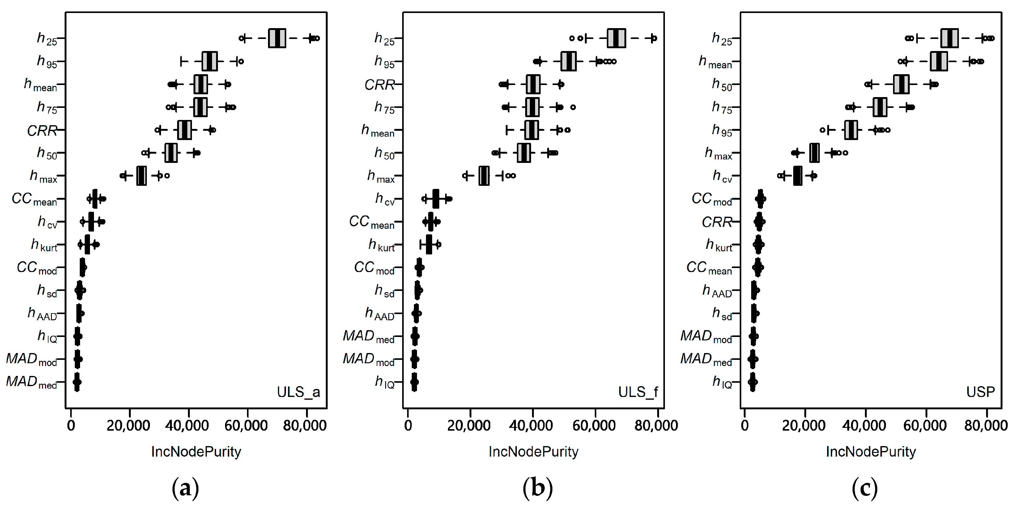
3.1. Feature Selection

The importance of the variables was determined using the RF model 1000 times. These boxplots, representing the importance of variables, show that seven variables were more important than the others for the different datasets (Figure 3). h25, h50, h75, h95, hmean, and hmax remained consistently important, while the CRR and hcv were different for the ULS and USP data. These seven variables, mainly height metrics, were selected as the predictor variables for the total and first ULS echoes and the point cloud of USP, separately (Table 6).
Boxplots of the selected variables from the three datasets are shown in Figure 4. The height percentiles become more similar as they increase. The point cloud values of USP are slightly higher and more concentrated than those of ULS when taking into account the boxplots of the lower height percentiles (h25 and h50) and hmean and of hcv and the CRR.

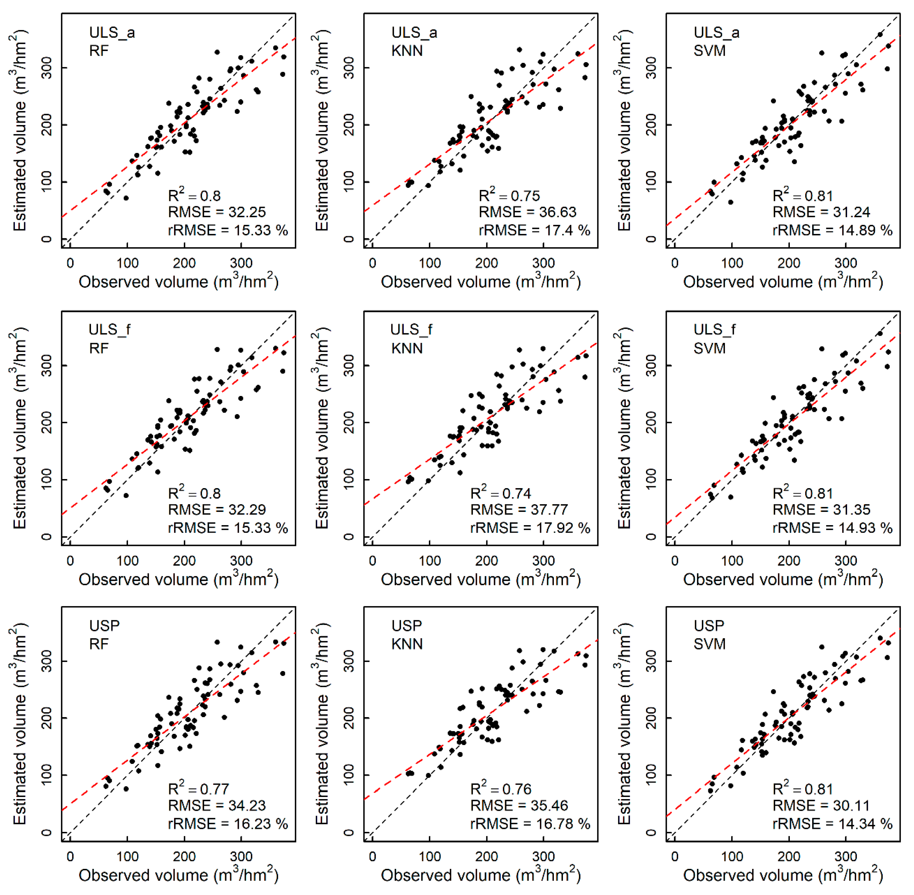
3.2. Growing Stock Volume Estimation

The selected variables of the three datasets were used as predictors to establish models for estimating growing stock volume. The hyper-parameters of the three machine learning models for estimation were tuned using 10-fold cross-validation (10 CV), with 30 repetitions, and are shown in Table 7. The best parameters of the RF and KNN algorithms were slightly different for the three datasets, while the best parameters of the SVM algorithms were similar.
Figure 5 shows the performances of the three machine learning algorithms for the three datasets. The predictions of growing stock volume had R2 values ranging from 0.74 to 0.81, the RMSE varied from 30.11 to 37.77 m3/hm2, and rRMSE spanned from 14.34% to 17.92%. The first returns of ULS performed as well as all the returns of ULS, with ΔR2 = −0.01–0, ΔRMSE = 0.04–1.14 m3/hm2, and ΔrRMSE = 0%–0.52%. USP achieved a similar accuracy to the ULS_a dataset, with R2 = 0.76–0.81, RMSE = 30.11–35.46 m3/hm2, and rRMSE = 14.34%–16.78%. In addition, among the three machine learning algorithms, SVM achieved the best results, with R2 = 0.81, RMSE = 30.11–31.35 m3/hm2, and rRMSE = 14.34%–14.93%, followed by RF, with R2 = 0.77–0.80, RMSE = 32.25–34.23 m3/hm2, and rRMSE = 15.33%–16.23%.

3.3. Effects of Point Density on Estimation Accuracy

Figure 6, Figure 7 and Figure 8 visually illustrate the effects of point density on the estimation accuracy of the ULS_a, ULS_f, and USP datasets, respectively. Overall, as the point density increases from 0.8 pts/m2 to 30 pts/m2, the estimation accuracy gradually improves and tends to stabilize. Table 8 presents the statistical values (mean estimation accuracy ± standard deviation) of estimation accuracy for the thinned point cloud data. For the different datasets, the results of ULS_a and ULS_f performed similarity at each point cloud density and for each estimation algorithm. This could be due to the small differences observed in the selected features derived from the ULS_a and ULS_f datasets. The influence of point density on the estimation accuracy of the USP dataset is minimal in terms of R2, RMSE, and rRMSE. For instance, the R2 of the thinned data ranged between 0.78 (±0.010) and 0.78 (±0.004), 0.74 (±0.012) and 0.76 (±0.015), and 0.81 (±0.004) and 0.81 (±0.001) for the RF, KNN, and SVM algorithms, respectively. Moreover, the standard deviation of R2, RMSE, and rRMSE for the different point densities derived from the USP dataset was lower than that from the ULS dataset; this may be due to the fact that the extracted point clouds from USP had a relatively short height.
Compared with the results of the RF and KNN estimation algorithms, the effects of point density on the estimation accuracy of the SVM model showed the least fluctuations for the three datasets. The R2 of the SVM algorithm ranged between 0.81 (±0.002) and 0.82 (±0.010), between 0.81 (±0.003) and 0.82 (±0.011), and between 0.81 (±0.001) and 0.81 (±0.004) for the ULS_a, ULS_f, and USP datasets. The R2 of the RF algorithm ranged from 0.77 (±0.021) to 0.79 (±0.009), from 0.78 (±0.019) to 0.81 (±0.004), and from 0.78 (±0.010) to 0.78 (±0.004) for the ULS_a, ULS_f, and USP datasets, respectively.
The estimation accuracies of the SVM became stable up to point densities of 5 pts/m2 and 0.8 pts/m2 for the ULS and USP datasets, respectively. The estimation accuracies of the RF algorithm increased as the point density increased, especially from 5 pts/m2 to 30 pts/m2. This indicates that the SVM was more stable than the other two algorithms, especially for the point cloud data with a low point density.

4. Discussion

4.1. Performances of Different Data Sources for Growing Stock Volume Estimation

The first and last returns were compared using ALS [36], through which it was found that the height metrics of the first + single returns were more stable than those of the last echo returns. There are few studies that compare the difference between the first and total returns. There were no significant differences between the estimation accuracies derived from the ULS first return and ULS total return data, which is mainly due to high point density, resulting in similar spatial distributions of their point cloud metrics, as demonstrated in Figure 4.
There were small differences between the estimation accuracies for the USP and ULS data in this study, which were comparable to previous findings. The predicted values of the forest structural attributes from the LiDAR point clouds were slightly better than those from USP [20,37]. The point cloud of stereo photogrammetry could achieve comparable results with those of LiDAR for estimating growing stock volume. Additionally, the estimation accuracies of growing stock volume using ULS or USP in this study were higher than those of using ALS or DAP acquired from a manned aircraft for conifer-dominated plantation forests [18,38]. Hawryło et al. [39] found the predicted value of DAP was similar to that of ALS for growing stock volume estimation for single-canopy-layer Scots pine-dominated stands, with rRMSEs of 15.2% and 17.0%–17.5% for ALS and DAP data, respectively.
Models derived from the USP point cloud metrics performed differently among the three machine learning algorithms and achieved a comparable accuracy to those of the ULS point cloud metrics using the SVM approach. Corte et al. [25] tested the ability of RF, SVM, an ANN, and XGBoost to estimate growing stock volume using ULS data and found that the SVM approach achieved the best performance. Although Fassnacht et al. [40] found that RF outperformed KNN and SVM for aboveground biomass estimation using ALS data, the interval of the predicted value for RF was larger than that of the SVM. The performance of RF among the different datasets in this study was similar. The SVM approach is more stable than the other non-parametric approaches for estimating forest structural attributes.
Additionally, the comparable performances of ULS and USP may, to some extent, also be explained by the vertical distribution of the 3D point clouds. LiDAR can acquire three-dimensional information about the observation target based on the time difference between the emission and return of laser pulses strongly penetrating the forest canopy, while DAP only represents the surface of the forest canopy, which may result in differences between the metrics generated from ALS- and DAP-based point clouds, especially for lower height percentiles and height statistical metrics (h25, hcv, and hmean). The differences in estimation accuracies between ULS and USP data determined by Cao et al. [41] is larger than that in this study, which may be caused by the different prediction methods and forest types. In their study, the prediction method was multiple regression and the difference in height metrics was more significant than that in this study.

4.2. The Effects on Growing Stock Volume Estimation Using Different Densities of Point Cloud Data

Some studies have focused on point density reductions for aboveground biomass [28], height estimation [42], DEM generation, and canopy metric accuracy [43] in different forest conditions using ALS point clouds. There are few studies on growing stock volume estimation for coniferous plantations using UAV point cloud datasets, especially using USP data. This study tried to analyze the influence of 3D point clouds with different point densities on growing stock volume estimation. The point density ranged from 0.8 pts/m2 to 30 pts/m2. To reduce the resampling influence on the thinned point clouds, this study randomly thinned the point clouds 30 times to reach a certain point density. The R2 intervals from a low to a high point density gradually reduced. This estimation accuracy at an increased point density agrees with a previous AGB estimation by Silva et al. [29], who concluded that AGB change estimates at the plot level are only slightly affected by pulse density, except at a very low point density of 0.2 pts/m2. Because of their efficiency, operability, and low cost, UAVs are a popular platform to acquire LiDAR data or photogrammetry images at a relatively low flight altitude, and they can produce point clouds with a high density. Therefore, the influence of point density on estimation accuracy must be explored to provide a solution to computational challenges, improve the efficiency of data acquisition, and cut procurement costs.
Compared with the RF model with different thinned point densities, the SVM model was more stable and had better accuracy. Since the SVM algorithm only uses the data points closest to the hyper-plane boundary, it is more suitable for datasets with a small training sample size. In addition, RF might be more sensitive to the metrics from point clouds with a relatively low point density.
In this study, the thinning method was mainly dependent on the pulse echoes. On the contrary, for the USP point clouds, there was no corresponding echo information, which means it can be considered a totally random thinning procedure. Due to the inability of photogrammetry to penetrate the forest canopy, image-based point clouds had a relatively shorter height interval than the point clouds of ULS.

4.3. The Effects on Growing Stock Volume Estimation Using Different Explanatory Variables

Seven metrics were selected as explanatory variables to estimate growing stock volume: h25, h50, h75, h90, the CRR, hmean, and hmax for the total or first echoes of the ULS data, and h25, h50, h75, h90, hcv, hmean, and hmax for the USP data, considering the importance of the predictors by random forest. The selected metrics included the height percentiles and height statistical and canopy cover metrics, which can be found in previous publications [25,41]. The height metrics extracted from the 3D point clouds had a strong correlation with forest stand height. According to the selected features, it is found that the height metrics are more sensitive to growing stock volume estimation. In general, the field growing stock volume was calculated using DBH and tree height with allometric equations. The difference between the selected features for the ULS and USP data are the CRR for ULS and hcv for USP. The CRR represents height distribution. hcv denotes the coefficient of point clouds with a height over 2 m. Actually, both these metrics could reflect the height distribution of point clouds to some extent. Because USP cannot penetrate through the forest canopy, the dense matching point cloud data are mainly concentrated in the upper portion [44]. The hcv of LiDAR point clouds is generally larger than that of image-based point clouds [45]. The height percentiles of ULS and USP became closer to each other as they increased, as demonstrated in previous studies [20,41].

4.4. Study Limitations

The explanatory variables were selected based on their importance values using random forest. There are many other methods that can be used to identify which variables should be inputted into models, such as those employed in previous publications [31,37,46]. However, there is still no widely accepted or standard method to determine which important features are the best explanatory variables. The required feature selection procedure for machine learning approaches is also not very clear. Feature selection depending on random forest has been applied for forest structural estimation [1,19], which is mainly attributed to RF having the ability to bootstrap. In addition, the effectiveness of thinned point clouds can be verified by obtaining data with different densities at different flight altitudes.

5. Conclusions

This study compared the performances of 3D point clouds obtained from USP and ULS data to estimate growing stock volume using three machine learning algorithms, namely RF, KNN, and SVM. USP can estimate growing stock volume with high accuracy. Among the three commonly used machine learning methods, SVM and RF can provide a higher estimation accuracy than KNN. SVM is also more stable than RF and KNN. The estimated growing stock volume using SVM and USP data combined with the DEM from ULS were also consistent with those from the ULS data. The estimation accuracy of the first echo ULS data was similar to that of the total echo ULS data in this coniferous plantation. Additionally, the point density had a slight influence on the estimated growing stock volume when using SVM for the ULS and USP data. SVM achieved relatively stable accuracies for ULS at a point density of up to 5 pts/m2 and at a low point density of 0.8 pts/m2 for USP. These findings are novel and can potentially be used for growing stock volume mapping, inventory keeping, and management.

Author Contributions

Conceptualization, Q.L.; data curation, M.L.; funding acquisition, Z.L.; methodology, M.L. and E.C.; supervision, Z.L. and Q.L.; visualization, M.L.; writing—original draft, M.L.; writing—review and editing, Z.L., Q.L. and E.C. All authors have read and agreed to the published version of the manuscript.

Funding

This work was supported in part by the Doctoral Research Start-up Fund Project of Shijiazhuang University (Project Number: 23BS038), Shijiazhuang Science and Technology Plan Project (Project Number: 231060201), and the National Natural Science Foundation of China (Project Number: 41871279).

Data Availability Statement

The original contributions presented in the study are included in the article, further inquiries can be directed to the corresponding author.

Acknowledgments

We are extremely grateful for the constructive comments and professional guidance from editors and reviewers on this article, which have been significantly helpful in the improvement of this study. Additionally, all the authors appreciate those who collected the field data and UAV data, and acknowledge the friendly support from the Wangyedian Forest Farm.

Conflicts of Interest

The authors declare no conflicts of interest.

References

  1. Leite, R.V.; Amaral, C.H.d.; Pires, R.d.P.; Silva, C.A.; Soares, C.P.B.; Macedo, R.P.; Silva, A.A.L.d.; Broadbent, E.N.; Mohan, M.; Leite, H.G. Estimating Stem Volume in Eucalyptus Plantations Using Airborne LiDAR: A Comparison of Area- and Individual Tree-Based Approaches. Remote Sens. 2020, 12, 1513. [Google Scholar] [CrossRef]
  2. Cui, H.; Liu, M. Analysis on the Results of the 9th National Forest Inventory. J. West China For. Sci. 2020, 5, 90–95. [Google Scholar]
  3. Wang, C. Biomass allometric equations for 10 co-occurring tree species in Chinese temperate forests. Forest Ecol. Manag. 2006, 222, 9–16. [Google Scholar] [CrossRef]
  4. Nilsson, M.; Nordkvist, K.; Jonzén, J.; Lindgren, N.; Axensten, P.; Wallerman, J.; Egberth, M.; Larsson, S.; Nilsson, L.; Eriksson, J.; et al. A nationwide forest attribute map of Sweden predicted using airborne laser scanning data and field data from the National Forest Inventory. Remote Sens. Environ. 2017, 194, 447–454. [Google Scholar] [CrossRef]
  5. Eisfelder, C.; Kuenzer, C.; Dech, S. Derivation of biomass information for semi-arid areas using remote-sensing data. Int. J. Remote Sens. 2012, 33, 2937–2984. [Google Scholar] [CrossRef]
  6. Cartus, O.; Kellndorfer, J.; Rombach, M.; Walker, W. Mapping Canopy Height and Growing Stock Volume Using Airborne Lidar, ALOS PALSAR and Landsat ETM+. Remote Sens. 2012, 4, 3320–3345. [Google Scholar] [CrossRef]
  7. Zhang, H.; Zhu, J.; Wang, C.; Lin, H.; Long, J.; Zhao, L.; Fu, H.; Liu, Z. Forest Growing Stock Volume Estimation in Subtropical Mountain Areas Using PALSAR-2 L-Band PolSAR Data. Forests 2019, 10, 276. [Google Scholar] [CrossRef]
  8. Beland, M.; Parker, G.; Sparrow, B.; Harding, D.; Chasmer, L.; Phinn, S.; Antonarakis, A.; Strahler, A. On promoting the use of lidar systems in forest ecosystem research. Forest Ecol. Manag. 2019, 450, 117484. [Google Scholar] [CrossRef]
  9. Görgens, E.B.; Packalen, P.; da Silva, A.G.P.; Alvares, C.A.; Campoe, O.C.; Stape, J.L.; Rodriguez, L.C.E. Stand volume models based on stable metrics as from multiple ALS acquisitions in Eucalyptus plantations. Ann. Forest Sci. 2015, 72, 489–498. [Google Scholar] [CrossRef]
  10. Packalen, P.; Strunk, J.; Packalen, T.; Maltamoa, M.; Mehtätalo, L. Resolution dependence in an area-based approach to forest inventory with airborne laser scanning. Remote Sens. Environ. 2019, 224, 192–201. [Google Scholar] [CrossRef]
  11. Dimitrios, P.; Azadeh, A.; Martin, S. 3D point cloud fusion from UAV and TLS to assess temperate managed forest structures. Int. J. Appl. Earth Obs. Geoinf. 2022, 112, 102917. [Google Scholar]
  12. Chen, X.; Wang, R.; Shi, W.; Li, X.; Zhu, X.; Wang, X. An Individual Tree Segmentation Method That Combines LiDAR Data and Spectral Imagery. Forests 2023, 14, 1009. [Google Scholar] [CrossRef]
  13. Persson, H.J.; Olofsson, K.; Holmgren, J. Two phase forest inventory using very high resolution laser scanning. Remote Sens. Environ. 2022, 271, 112909. [Google Scholar] [CrossRef]
  14. Chan, E.P.Y.; Fung, T.; Wong, F.K.K. Estimating above-ground biomass of subtropical forest using airborne LiDAR in Hong Kong. Sci. Rep. 2021, 11, 1751. [Google Scholar] [CrossRef] [PubMed]
  15. Goodbody, T.R.H.; Coops, N.C.; White, J.C. Digital Aerial Photogrammetry for Updating Area-Based Forest Inventories: A Review of Opportunities, Challenges, and Future Directions. Curr. For. Rep. 2019, 5, 55–75. [Google Scholar] [CrossRef]
  16. Iqbal, I.A.; Musk, R.A.; Osborn, J.; Stone, C.; Lucieer, A. A comparison of area-based forest attributes derived from airborne laser scanner, small-format and medium-format digital aerial photography. Int. J. Appl. Earth Obs. Geoinf. 2019, 76, 231–241. [Google Scholar] [CrossRef]
  17. Næsset, E.; Gobakken, T.; Jutras-Perreault, M.-C.; Ramtvedt, E.N. Comparing 3D Point Cloud Data from Laser Scanning and Digital Aerial Photogrammetry for Height Estimation of Small Trees and Other Vegetation in a Boreal–Alpine Ecotone. Remote Sens. 2021, 13, 2469. [Google Scholar] [CrossRef]
  18. Vastaranta, M.; Wulder, M.A.; White, J.C.; Pekkarinen, A.; Tuominen, S.; Ginzler, C.; Kankare, V.; Holopainen, M.; Hyyppä, J.; Hyyppä, H. Airborne laser scanning and digital stereo imagery measures of forest structure: Comparative results and implications to forest mapping and inventory update. Can. J. Remote Sens. 2013, 39, 382–395. [Google Scholar] [CrossRef]
  19. Tompalski, P.; White, J.C.; Coops, N.C.; Wulder, M.A. Quantifying the contribution of spectral metrics derived from digital aerial photogrammetry to area-based models of forest inventory attributes. Remote Sens. Environ. 2019, 234, 111434. [Google Scholar] [CrossRef]
  20. Navarro, J.A.; Fernández-Landa, A.; Tomé, J.L.; Guillén-Climent, M.L.; Ojeda, J.C. Testing the quality of forest variable estimation using dense image matching: A comparison with airborne laser scanning in a Mediterranean pine forest. Int. J. Remote Sens. 2018, 39, 4744–4760. [Google Scholar] [CrossRef]
  21. Puliti, S.; Solberg, S.; Granhus, A. Use of UAV Photogrammetric Data for Estimation of Biophysical Properties in Forest Stands Under Regeneration. Remote Sens. 2019, 11, 233. [Google Scholar] [CrossRef]
  22. Sadeepa, J.; Toshiaki, O.; Satoshi, T. Evaluating the Performance of Photogrammetric Products Using Fixed-Wing UAV Imagery over a Mixed Conifer–Broadleaf Forest: Comparison with Airborne Laser Scanning. Remote Sens. 2018, 10, 187. [Google Scholar] [CrossRef]
  23. Guimarães, N.; Pádua, L.; Marques, P.; Silva, N.; Peres, E.; Sousa, J.J. Forestry Remote Sensing from Unmanned Aerial Vehicles: A Review Focusing on the Data, Processing and Potentialities. Remote Sens. 2020, 12, 1046. [Google Scholar] [CrossRef]
  24. Liu, K.; Shen, X.; Cao, L.; Wang, G.; Cao, F. Estimating forest structural attributes using UAV-LiDAR data in Ginkgo plantations. ISPRS J. Photogramm. 2018, 146, 465–482. [Google Scholar] [CrossRef]
  25. Corte, A.P.D.; Souza, D.V.; Rex, F.E.; Sanquetta, C.R.; Broadbent, E.N. Forest inventory with high-density UAV-Lidar: Machine learning approaches for predicting individual tree attributes. Comput. Electron. Agric. 2020, 179, 105815. [Google Scholar] [CrossRef]
  26. Zhang, B.; Li, X.; Du, H.; Zhou, G.; Mao, F.; Huang, Z.; Zhou, L.; Xuan, J.; Gong, Y.; Chen, C. Estimation of Urban Forest Characteristic Parameters Using UAV-Lidar Coupled with Canopy Volume. Remote Sens. 2022, 14, 6375. [Google Scholar] [CrossRef]
  27. Teshome, F.T.; Bayabil, H.K.; Hoogenboom, G.; Schaffer, B.; Singh, A.; Ampatzidis, Y. Unmanned aerial vehicle (UAV) imaging and machine learning applications for plant phenotyping. Comput. Electron. Agric. 2023, 212, 108064. [Google Scholar] [CrossRef]
  28. Garcia, M.; Saatchi, S.S.; Ferraz, A.; Silva, C.A.; Ustin, S.L.; Koltunov, A.; Balzter, H. Impact of data model and point density on aboveground forest biomass estimation from airborne LiDAR. Carbon Bal. Manag. 2017, 12, 4. [Google Scholar] [CrossRef] [PubMed]
  29. Silva, C.A.; Hudak, A.; Vierling, L.A.; Klauberg, C.; García, M.; Ferraz, A.; Keller, M.; Eitel, J.; Saatchi, S. Impacts of Airborne Lidar Pulse Density on Estimating Biomass Stocks and Changes in a Selectively Logged Tropical Forest. Remote Sens. 2017, 9, 1068. [Google Scholar] [CrossRef]
  30. He, C. The Key Technology for Precision Measurement in Forest Surveying. Ph.D. Thesis, Beijing Forestry University, Beijing, China, 2013. [Google Scholar]
  31. Navarro, J.A.; Tomé, J.L.; Marino, E.; Guillén-Climent, M.L.; Fernández-Landa, A. Assessing the transferability of airborne laser scanning and digital aerial photogrammetry derived growing stock volume models. Int. J. Appl. Earth Obs. Geoinf. 2020, 91, 102135. [Google Scholar] [CrossRef]
  32. Breiman, L. Random Forests. Mach. Learn. 2001, 45, 5–32. [Google Scholar] [CrossRef]
  33. Domingo, D.; Lamelas, M.T.; Montealegre, A.L.; García-Martín, A.; Riva, J.d.l. Estimation of Total Biomass in Aleppo Pine Forest Stands Applying Parametric and Nonparametric Methods to Low-Density Airborne Laser Scanning Data. Forests 2018, 9, 158. [Google Scholar] [CrossRef]
  34. Li, M.; Li, Z.; Liu, Q.; Chen, E. Comparison of Coniferous Plantation Heights Using Unmanned Aerial Vehicle (UAV) Laser Scanning and Stereo Photogrammetry. Remote Sens. 2021, 13, 2885. [Google Scholar] [CrossRef]
  35. Tompalski, P.; Coops, N.C.; White, J.C.; Goodbody, T.R.H.; Hennigar, C.R.; Wulder, M.A.; Socha, J.; Woods, M.E. Estimating Changes in Forest Attributes and Enhancing Growth Projections: A Review of Existing Approaches and Future Directions Using Airborne 3D Point Cloud Data. Curr. For. Rep. 2021, 7, 1–24. [Google Scholar] [CrossRef]
  36. Næsset, E. Effects of different sensors, flying altitudes, and pulse repetition frequencies on forest canopy metrics and biophysical stand properties derived from small-footprint airborne laser data. Remote Sens. Environ. 2009, 113, 148–159. [Google Scholar] [CrossRef]
  37. Noordermeer, L.; Bollandsås, O.M.; Ørka, H.O.; Næsset, E.; Gobakken, T. Comparing the accuracies of forest attributes predicted from airborne laser scanning and digital aerial photogrammetry in operational forest inventories. Remote Sens. Environ. 2019, 226, 26–37. [Google Scholar] [CrossRef]
  38. Nurminen, K.; Karjalainen, M.; Yu, X.; Hyyppae, J.; Honkavaara, E. Performance of dense digital surface models based on image matching in the estimation of plot-level forest variables. ISPRS J. Photogramm. 2013, 83, 104–115. [Google Scholar] [CrossRef]
  39. Hawryło, P.; Tompalski, P.; Wężyk, P. Area-based estimation of growing stock volume in Scots pine stands using ALS and airborne image-based point clouds. Forestry 2017, 90, 686–696. [Google Scholar] [CrossRef]
  40. Fassnacht, F.E.; Hartig, F.; Latifi, H.; Berger, C.; Hernandez, J.; Corvalan, P.; Koch, B. Importance of sample size, data type and prediction method for remote sensing-based estimations of aboveground forest biomass. Remote Sens. Environ. 2014, 154, 102–114. [Google Scholar] [CrossRef]
  41. Cao, L.; Liu, H.; Fu, X.; Zhang, Z.; Ruan, H. Comparison of UAV LiDAR and Digital Aerial Photogrammetry Point Clouds for Estimating Forest Structural Attributes in Subtropical Planted Forests. Forests 2019, 10, 145. [Google Scholar] [CrossRef]
  42. Jakubowski, M.K.; Guo, Q.; Kelly, M. Tradeoffs between lidar pulse density and forest measurement accuracy. Remote Sens. Environ. 2013, 130, 245–253. [Google Scholar] [CrossRef]
  43. Hansen, E.; Gobakken, T.; Næsset, E. Effects of Pulse Density on Digital Terrain Models and Canopy Metrics Using Airborne Laser Scanning in a Tropical Rainforest. Remote Sens. 2015, 7, 8453–8468. [Google Scholar] [CrossRef]
  44. Chen, S.; McDermid, G.J.; Castilla, G.; Linke, J. Measuring Vegetation Height in Linear Disturbances in the Boreal Forest with UAV Photogrammetry. Remote Sens. 2017, 9, 1257. [Google Scholar] [CrossRef]
  45. White, J.C.; Coops, N.C.; Wulder, M.A.; Vastaranta, M.; Hilker, T.; Tompalski, P. Remote Sensing Technologies for Enhancing Forest Inventories: A Review. Can. J. Remote Sens. 2016, 42, 619–641. [Google Scholar] [CrossRef]
  46. Li, Y.C.; Li, C.; Li, M.; Liu, Z. Influence of Variable Selection and Forest Type on Forest Aboveground Biomass Estimation Using Machine Learning Algorithms. Forests 2019, 10, 1073. [Google Scholar] [CrossRef]
Figure 1. The location of the study area (a). The spatial distribution of the ULS flight sites (b).
Forests 16 00663 g001
Figure 2. An actual photo of Larix principis-rupprechtii plantations.
Forests 16 00663 g002
Figure 3. Importance of variables for growing stock volume estimation using the RF algorithm for 1000 iterations. All echoes of ULS (a), first echo of ULS (b), and point cloud of USP (c).
Forests 16 00663 g003
Figure 4. The boxplots of the selected variables for the three datasets. ULS_a represents all the echoes of ULS, ULS_f represents the first echo of ULS, and USP represents the point cloud of USP.
Forests 16 00663 g004
Figure 5. Scatterplots of predicted volume and observed volume using three machine learning algorithms for three datasets (the black dashed line is 1:1 fitting line, the red dashed line is the fitting line of predicted volume and observed volume).
Forests 16 00663 g005
Figure 6. Estimation accuracies of growing stock volume according to three machine learning algorithms for all echoes of ULS at different point densities.
Forests 16 00663 g006
Figure 7. Estimation accuracies of growing stock volume according to three machine learning algorithms for first echo of ULS at different point densities.
Forests 16 00663 g007
Figure 8. Estimation accuracies of growing stock volume according to three machine learning algorithms for point cloud of USP at different point densities.
Forests 16 00663 g008
Table 1. Volume equations of different tree species.
SpeciesDuality Volume Equation
Larix principis-rupprechtii 10 ( 3.49890 + 2.75504 × log 10 DBH 0.39405 × l o g 10 D B H 2 1.37915 × l o g 10 h + 1.14586 × l o g 10 h 2 )
Pinus tabuliformis 2.53309 × 10 5 × D B H 2 × h 8.57378 × 10 7 × D B H 3 × h 6.00033 × 10 5 × D B H 2 + 2.93720 × 10 5 × D B H 2 × h × l o g 10 D B H
Table 2. Summary description of each plot.
Forest CasesMinimumMedianMeanMaximumSD
DBH (cm)7.714.015.231.24.7
Lorey’s height (m)6.812.813.420.83.5
Growing stock volume (m3/hm2)62.4206.4209.7374.470.7
Table 3. The specifications of the ULS and USP systems.
ULSUSP
UAV ModelRC6-2000UAV ModelDJI Phantom 4 RTK
LiDAR modelRiegl VUX-1Camera modelCMOS
Laser wavelengthNear-infraredCMOS size36.0 mm × 24.0 mm
Scan patternRotate MirrorFOVHorizonal 70° Vertical ± 10°
Echoes2Pixel unit4.1 µm × 4.1 µm
Range3 m–920 mRotor3
Rotor8Pixels50,320,896
PRF10 Hz–200 HzImage size4864 × 3648 pixels
Laser divergence3 mradFocal length8.8 mm
Scan FOV30° × 360°BandsR/G/B
Max scan frequency20 Hz
Vertical accuracy<5 cm
Table 4. The features extracted from the point clouds of ULS and USP.
CategoryParametersDescription
Height percentilesh25, h50, h75, h95Height percentiles for point cloud above 2 m
Height statistical metricshmaxMaximum value for point cloud above 2 m
hmeanMean value for point cloud above 2 m
hcvCoefficient of variation for point cloud above 2 m
hsdStandard deviation for point cloud above 2 m
hIQh75h25
hkurtHeight kurtosis for point cloud above 2 m
hAADAverage absolute deviation
MADmedMedian of the absolute deviations from the overall median
MADmodMedian of the absolute deviations from the overall mode
Canopy density metricsCRR(hmeanhmin) / (hmaxhmin)
CCmeanPercentage of points above the mean of heights
CCmodPercentage of points above the mode of heights
Table 5. The key parameters for each machine learning algorithm and the tuned ranges.
AlgorithmKey ParametersTune Interval
RFmtry2, 3, 4, 5, 6, 7
KNNk1, 2, 3, 4, 5, 6, 7
SVMcost2, 4, 6, 8, 10, 20, 30, 40, 50, 60, 80, 100
sigma0.015, 0.02, 0.05, 0.1, 0.15, 0.2, 0.5, 1
Table 6. The selected metrics of the three datasets.
DatasetsDatasetsThe Selected Variables
ULS_aAll echoes of ULSh25, h50, h75, h95, hmean, hmax, CRR
ULS_fThe first echoes of ULSh25, h50, h75, h95, hmean, hmax, CRR
USPPoint cloud of USPh25, h50, h75, h95, hmean, hmax, hcv
Table 7. The best parameters of the three algorithms using the selected metrics.
DatasetsRFKNNSVM
ULS_amtry = 2k = 5sigma= 0.015, cost = 20
ULS_fmtry = 3k = 6sigma= 0.015, cost = 20
USPmtry = 6k = 7sigma= 0.015, cost = 10
Table 8. The statistical values (mean estimation accuracy ± standard deviation) of estimation accuracy for the thinned point cloud data.
DatasetPoint
Density
RFKNNSVM
R2RMSErRMSE/
%
R2RMSErRMSE/
%
R2RMSErRMSE/
%
ULS_a0.80.77 ± 0.02133.93 ± 1.02516.11 ± 0.4880.77 ± 0.01535.49 ± 0.78316.85 ± 0.3520.82 ± 0.01030.45 ± 0.66914.51 ± 0.310
10.77 ± 0.01934.07 ± 1.01916.18 ± 0.4850.77 ± 0.01235.43 ± 0.68516.81 ± 0.3110.82 ± 0.01030.34 ± 0.55214.45 ± 0.258
50.77 ± 0.01033.63 ± 0.66315.97 ± 0.3140.76 ± 0.00736.02 ± 0.45517.1 ± 0.2190.81 ± 0.00430.61 ± 0.31914.58 ± 0.157
100.79 ± 0.00832.7 ± 0.50315.52 ± 0.2410.76 ± 0.00835.94 ± 0.43417.05 ± 0.2030.81 ± 0.00330.70 ± 0.25214.62 ± 0.122
300.79 ± 0.00932.11 ± 0.62615.24 ± 0.2960.77 ± 0.00735.54 ± 0.35116.86 ± 0.1680.81 ± 0.00230.82 ± 0.17114.69 ± 0.086
ULS_f0.80.78 ± 0.01933.67 ± 0.98615.99 ± 0.4670.77 ± 0.01435.55 ± 0.71116.88 ± 0.3190.82 ± 0.01230.6 ± 0.75614.58 ± 0.359
10.78 ± 0.02233.83 ± 1.17116.06 ± 0.5590.77 ± 0.01335.56 ± 0.74716.88 ± 0.3380.82 ± 0.01130.56 ± 0.67014.55 ± 0.315
50.79 ± 0.01133.00 ± 0.68515.67 ± 0.3260.76 ± 0.01136.15 ± 0.64717.15 ± 0.3010.81 ± 0.00730.79 ± 0.37014.66 ± 0.181
100.80 ± 0.01032.13 ± 0.56715.25 ± 0.2710.76 ± 0.00936.19 ± 0.44217.17 ± 0.1990.81 ± 0.00430.78 ± 0.29314.65 ± 0.143
300.81 ± 0.00431.46 ± 0.26514.92 ± 0.1290.77 ± 0.00735.78 ± 0.44116.98 ± 0.2090.81 ± 0.00330.87 ± 0.22814.7 ± 0.113
USP0.80.78 ± 0.01033.23 ± 0.64415.74 ± 0.3200.74 ± 0.01235.63 ± 0.69916.86 ± 0.3290.81 ± 0.00430.06 ± 0.33014.32 ± 0.161
10.78 ± 0.01133.26 ± 0.64915.75 ± 0.3200.75 ± 0.01435.4 ± 0.82716.76 ± 0.3860.81 ± 0.00429.97 ± 0.34014.28 ± 0.165
50.78 ± 0.00633.17 ± 0.39815.71 ± 0.1950.74 ± 0.01735.62 ± 1.0616.87 ± 0.5030.81 ± 0.00330.06 ± 0.20014.33 ± 0.097
100.78 ± 0.00633.09 ± 0.43215.67 ± 0.210.74 ± 0.01735.76 ± 0.90416.94 ± 0.4280.81 ± 0.00230.00 ± 0.13914.30 ± 0.067
300.78 ± 0.00433.85 ± 0.20016.07 ± 0.0930.76 ± 0.01535.33 ± 0.54416.73 ± 0.2630.81 ± 0.00130.00 ± 0.09814.30 ± 0.047
Disclaimer/Publisher’s Note: The statements, opinions and data contained in all publications are solely those of the individual author(s) and contributor(s) and not of MDPI and/or the editor(s). MDPI and/or the editor(s) disclaim responsibility for any injury to people or property resulting from any ideas, methods, instructions or products referred to in the content.

