Article

Elevational Distribution of Ants Across Seasons in a Subtropical Rainforest of Eastern Australia

1
Yunnan Key Laboratory of Forest Ecosystem Stability and Global Change Response, Xishuangbanna Tropical Botanical Garden, Chinese Academy of Sciences, Menglun 666303, China
2
University of Chinese Academy of Sciences, No. 19A Yuquan Road, Beijing 10049, China
3
Biodiversity and Geosciences, Queensland Museum, Brisbane, QLD 4101, Australia
4
School of Environment and Science, Griffith University, Brisbane, QLD 4111, Australia
5
School of Biological Sciences, The University of Hong Kong, Hong Kong SAR, China
6
Center of Plant Ecology, Core Botanical Gardens, Chinese Academy of Sciences, Mengla 666303, China
*
Author to whom correspondence should be addressed.
Forests 2025, 16(4), 664; https://doi.org/10.3390/f16040664
Submission received: 6 March 2025 / Revised: 3 April 2025 / Accepted: 4 April 2025 / Published: 10 April 2025

Abstract

:
Elevational gradients are widely studied to understand environmental variability and species distribution. Ants play vital roles in ecosystems and are frequently included in elevational biogeography studies. Despite their ecological importance and well-documented elevational patterns, little is known about their temporal variability across elevations. We surveyed ground and arboreal ants in austral summer, autumn, spring, and winter in a subtropical rainforest of Lamington National Park, Queensland, Australia. Given their physiological and microhabitat differences, ground and arboreal ants may exhibit distinct spatiotemporal patterns. Using litter extraction for ground ants and bark spraying for arboreal ants, we collected 14,916 individuals from 124 species. Species richness and abundance were lowest in austral winter, particularly for arboreal ants. Both richness and abundance declined with elevation, and this pattern remained consistent across seasons. While seasonal and elevational differences significantly influenced species composition, seasonal variation did not cause major shifts in the elevational distribution of ground or arboreal ants. A total of 43 species were identified as indicators of specific elevations, with species such as Notoncus capitatus and Colobostruma biconvexa being specialists of low elevations, and undescribed Monomorium and Discothyrea species being specialists of high elevations. In contrast, only two species were identified as seasonal indicators, which were undescribed Tapinoma and Anonychomyrma species, specialists of the warm season. Our findings suggest that ants reduce activity in winter but maintain stable elevational distributions regardless of season or microhabitat use, making their distributions a reliable indicator of their climatic niches.

1. Introduction

Understanding the spatiotemporal patterns of organisms is crucial for community ecology [1,2]. Spatially structured factors like climate, habitat characteristics, and resource availability strongly influence species distribution and abundance at different scales. On a large scale, biodiversity is highest near the tropics and decreases towards the poles [3], patterns likely to be explained by temperature, precipitation, and productivity gradients [4]. However, elucidating how species assembly is shaped by spatiotemporal factors using latitudinal gradients is challenging, as observing latitudinal patterns requires regional- or global-scale studies [5]. In addition, large-scale studies that rely on environmental data may miss crucial mechanisms such as species interactions and how environmental heterogeneity at the local scale shapes diversity patterns [6]. Smaller scales like elevational gradients offer better access to study spatiotemporal factors influencing biodiversity [7,8]. Temperature decreases faster with elevation than latitude, forming sharper environmental changes [9,10]. Korner [7] highlighted this using elevational gradients in ecological research, addressing the importance of microhabitat–climate relations in their analyses, while Sundqvist et al. [11] also addressed elevational gradients as powerful natural experiments for studying community and ecosystem responses to climate change.
Rahbek [12] and Kessler et al. [13] reviewed elevational studies and revealed that species richness generally decreases with elevation, akin to latitudinal gradients. However, Rahbek emphasized considering area effects on diversity along the gradients, which often leads to hump-shaped diversity patterns. More recent studies have shown that other factors, such as productivity, also play important roles in shaping species diversity because productivity typically peaks at mid-elevations, which is linked to the formation of hump-shaped diversity patterns [14,15]. However, species richness and compositional patterns along elevational ranges vary by taxa and their associated traits [16,17]. For instance, plant species often show a mid-elevation peak in diversity due to optimal conditions for growth and reproduction [7]. Vertebrates, such as birds and mammals, may display varied responses, with some species richness peaking at lower elevations, while others peak at mid-elevations, where a combination of factors like temperature and habitat complexity is favorable [18]. Invertebrates, including insects, frequently exhibit a range of diversity patterns depending on their ecological niches and life history traits [19]. Ants, for example, show monotonic declines in species richness with increasing elevation but often exhibit mid-elevation peaks, a pattern that may be influenced by factors such as habitat structure, temperature, species interactions, and resource availability [20,21,22,23,24].
Elevational studies often overlook the importance of incorporating temporal dynamics like seasonality, especially in relation to insects. Seasonality plays a crucial role in shaping insect behavior, metabolism, phenology, and distribution patterns. For example, some insects enter diapause, which temporarily pauses their development during colder climates [25], ultimately impacting ecosystem-wide organism distribution patterns. Considering the seasonal dynamics of organisms is essential for understanding how elevation influences biodiversity patterns. Maicher et al. [26] examined shifts in Lepidoptera (moths and butterflies) distributions along elevational gradients, focusing on how seasonal changes in resource availability drive these patterns. They demonstrated that Lepidoptera diversity peaked at different elevations depending on the season, likely due to fluctuations in food resources and climatic conditions at various elevations. Such seasonal migrations or elevational shifts highlight the importance of incorporating temporal factors when assessing biodiversity responses to elevation. The study of the seasonality of insects shows that their pattern of seasonality varies for different groups of insects [27]. Recent studies have shown that insects like Lepidoptera [26] and Coleoptera [28] shift their elevational distribution to follow preferred climate conditions and resources. However, eusocial insects like ants were found to have less pronounced seasonality than other insects due to their capacity to control the temperature within their colonies and access to a diverse array of food sources [29].
Vertical variation in biodiversity patterns, such as differences between the ground and canopy layers, significantly influences local-scale diversity across geographic and temporal gradients. Scheffers et al. [30] highlighted that forest vertical strata present steeper gradients than latitude and elevation. Subsequent studies have emphasized the role of vertical microclimate variation on the distribution patterns of insects [31,32]. The forest canopy generally experiences harsher climatic conditions compared to the understory [33]. The tree structure moderates climatic factors like humidity and temperature from the canopy to the ground, resulting in more stable climates on the forest floor [34]. This vertical stratification affects biodiversity patterns, such as in insects, and is also observed along latitudinal and elevational gradients [33]. A recent study found a temperature difference of up to 5 °C within just three meters of forest height [31]. Therefore, arboreal species face higher climatic variation and often exhibit greater resilience to climate change than ground species, as evidenced by arboreal ants’ wider elevational range [31]. Conversely, ground species may be more sensitive to seasonal climatic changes due to their adaptations to more stable conditions on the forest floor, as observed in the Brazilian Cerrado [35]. A recent study also showed that ground ants are more sensitive to elevational changes, as ground ants have a higher turnover rate along the elevational gradient than arboreal ants [32]. Studies indicate that seasonal variations in resource availability are crucial in shaping biodiversity patterns, especially for arboreal species. Basset et al. [36], for example, found that insect diversity was generally higher in the canopy compared to the understory, though this pattern varied across seasons. This suggests that vertical stratification and seasonal dynamics interact to shape biodiversity, with the canopy and forest floor layers potentially responding differently to seasonal resource changes.
In this study, we aim to investigate how ant species richness and composition vary between ground and arboreal habitats along elevational gradients in a subtropical rainforest of southeast Queensland, Australia, and whether their distributions shift with the seasons. We hypothesize that the diversity and community composition of ants are elevationally stratified with monotonic decreases in diversity with increasing elevation [37]. Due to the eusocial nature of ants, we hypothesize that seasonal influence does not shift their elevational distributions. As arboreal ants are adapted to climatic variability [32], the effects of both elevation and season are weaker for arboreal ants over ground ants.

2. Materials and Methods

2.1. Methodology Overview

The study site was located in the subtropical rainforest of Lamington National Park (28°08′52.0″ S, 153°08′13.0″ E–28°15′43.0″ S, 153°10′11.0″ E), which encompasses a large tract of undisturbed forests [38]. The study areas covered various elevations ranging from approximately 300 to 1100 m above sea level (m a.s.l.). At the Green Mountains section of Lamington National Park, we established 20 plots at five elevation bands (300, 500, 700, 900, and 1100 m a.s.l.) along the single elevational transect. Four 20 m × 20 m experimental plots were established in each elevation band. Plots within each elevational band were located at similar elevations (within ± 75 m a.s.l. from each elevational band) and at least 400 m away from each other. Each plot was surveyed across multiple seasons in the austral spring (October 2006), summer (January–February 2008), autumn (March 2007), and winter (July 2007) to capture seasonal variations in ant communities. For more details on the plot design, see Kitching et al. [38].
At the lowest elevation of the study site (300 m), the forest contains the Araucaria complex notophyll vine forest, including Araucaria cunninghamii [39]. The mid-elevations of this study site (500–900 m a.s.l.) consist of a complex notophyll vine forest. A cool temperate microphyll fern forest, in which Nothofagus moorei is the dominant species, occupies the highest elevation (1100 m a.s.l.) [39]. The study area exhibits distinct seasonal climate patterns, with a warmer, wetter period from November to March and a cooler, drier period from April to October [40]. At the Green Mountains section of Lamington National Park (approximately 940 m a.s.l.), average air temperatures range from a winter minimum of 4 °C to a summer maximum of 27 °C. Annual rainfall averages 1827 mm, with some months exceeding 200 mm. However, precipitation declines significantly in July, falling below 100 mm. The driest month is September, with an average of around 60 mm, followed by a gradual increase in rainfall beginning in October. Temperature across the study area generally decreases as elevation increases. At lower elevations (around 300 m a.s.l.), temperatures can exceed 35 °C in the warmer months, while higher elevations (above 1000 m a.s.l.) may experience temperatures near or below 0 °C during cooler periods [40]. During the summer, humidity levels were consistently high at 1100 m a.s.l., with moist conditions persisting for longer durations compared to lower elevations. This elevation experiences prolonged periods of elevated humidity, particularly during daytime, indicating more stable and humid microclimatic conditions. According to Strong et al. [40], the soil across all the plots originated from tertiary basaltic rocks, which exhibit characteristics of loam-to-silty-clay loam, identified as Krasnozem Gn4.11 or Gn4.12 in the Northcote classification [41] and categorized as Ferralsol according to the FAO classification [42].

2.2. Ant Sampling

We captured ground and arboreal ants using litter extraction and bark spray, respectively. Although there were some species (e.g., Monomorium spp.) that were found in both litter extraction and bark spray, we did not exclude such species from either litter extraction or bark spray samples, as it is difficult to determine which species are truly ground- or arboreal-active species. As our sampling methods do not necessarily capture ant colonies, we intended to measure ant activity at the time of sampling.

2.3. Litter Extraction

We collected litter and loose topsoil from 2 m2 at each plot. A metal frame measuring 50 × 50 cm (0.25 m2) was used to collect samples from the areas just outside the 20 × 20 m plot areas (this was performed to avoid disturbances in the area where plant diversity and soil properties were measured). Two sets of four 0.25 m2 samples were taken from opposite sides of each plot, at least five meters away from each other. Litter and loose soil were collected by hand and placed into a sifting bag with a hexagonal mesh made of chicken wire to separate large leaf and other organic materials while allowing small pieces of litter and ants to fall through the mesh. Due to the mountain’s topography and the litter quality, the sampling area was selected non-randomly (areas with adequate accessible litter without signs of rain-washing). The litter was then transferred to a cloth bag brought back to the field laboratory. Samples were transferred to Tullgren funnels with a 60-watt incandescent bulb. Usually, the operation of the Tullgren is 24 h for dry litter, but we used 36 h for the wetter litter. All insect samples were kept in ethanol.

2.4. Bark Spray

Arboreal ants were collected outside the 20 × 20 m quadrat from 10 large trees (diameter at breast height > 30 cm). Two sets of five trees were selected from opposite sides of each plot. On each tree, we sprayed pyrethroid insecticide in cans from the base of the tree up to the highest possible position the spray could reach (approximately 3 m high from the ground). Five rectangular sheets (rip-stop nylon, measuring 160 cm × 105 cm) were placed at the base of the trees to collect falling insects. Approximately 15 min after spraying, the rectangular sheets were carefully collected, and all insects were transferred to a vial with ethanol. For more details, see Burwell and Nakamura’s study [37].

2.5. Sorting and Identification

All ant workers and egatoid queen individuals were identified to described genera and species whenever possible. This was accomplished by referring to the available published taxonomic literature, comparing specimens to type specimens from the Australian National Insect Collection and Queensland Museum and consulting with specialists on certain ant genera, such as Monomorium expert Brian Heterick and Polyrhachis expert Rudy Kohout. Any specimens that could not be definitively identified to species were assigned a morphospecies code for use in the analyses and for future identification efforts. The classification of the ants to the family and genus level followed the taxonomic frameworks provided by Bolton [43] and Shattuck and Barnett [44], respectively. All specimen vouchers have been deposited and are being maintained in the Queensland Museum collection.

2.6. Data Analysis

The sampling unit of the analysis was ants collected from each plot across the four seasons (four plots from each of the five elevational bands collected across the four seasons, N = 80). We analyzed ants collected by litter extraction and bark spray separately, as they represent ground and arboreal foraging ants, respectively. We calculated abundance scores for ants using the 8-point scale transformation proposed by Hoffmann and Kay [45] as follows: 1 = 1 individual; 2 = 2–5; 3 = 6–10; 4 = 11–20; 5 = 21–50; 6 = 51–100; 7 = 101–200; and 8 ≥ 200. This point-scaling was used because ants are eusocial, and we accounted for the chances of collecting ants near their colony or when they were grouped to capture and transfer prey. All statistical analyses described below were performed with the software R v. 4.2.2 [46], and results were visualized with the ggplot2 package [47].
We first calculated the gamma diversity of ants and assessed the sampling effectiveness for the ground and arboreal ants across seasons with the iNEXT package [48]. Species accumulation curves were generated with Hill number q = 0 (species richness) and the sample coverage of ants collected from the four seasons was calculated. We extrapolated the data by doubling the number of samples with 100 bootstrapping replications to estimate 95% confidence intervals [48,49].
We fitted generalized linear mixed models (GLMMs) using the glmmTMB package [50] to investigate the effects of elevation and season on ant species richness and total abundance scores (i.e., the sum of abundance scores of the species collected in each sampling unit). We considered elevation (five elevational bands), season (four seasons), and their interaction as fixed effects and included plots as a random factor to account for the repeated seasonal sampling from the same plot. We fitted ant species richness and abundance score data assuming a Poisson distribution of residuals with a log link function. We tested overdispersion in the models using the check_overdispersion() function in the performance package [51]. When overdispersion was detected, we fitted the data using the negative binomial distribution (nbinom2). The significance of elevation, season, and their interaction was assessed by calculating chi-squared values from type II analysis of variance tables generated by the Anova() function in the car package [52]. We performed post hoc pairwise comparisons of the estimated marginal means using the emmeans() function from the emmeans package [53].
We assessed whether seasonal influences altered beta diversity across the elevations. We used the betapart package [54] to calculate the turnover and nestedness components of beta diversity based on the Jaccard index (presence/absence of ant species) [55] across the four seasons within each sampling plot. We then tested whether beta turnover and nestedness values changed across the elevational bands using the same GLMMs and post hoc tests as described above, except we fitted the models using a beta distribution of residuals. As the beta distribution cannot accept 0 or 1, we added a very small value (0.0001) to all of the data so that we were able to include one plot that had 0.
We also assessed whether individual ant species showed consistent or shifting elevational patterns across seasons. We applied the same GLMMs and post hoc comparisons as described above for species richness and abundance scores. We used ant species that occurred in at least four sampling units in each season. To visualize their elevational distributions across the seasons, we used the geom_density() function in the ggplot2 package to draw the kernel density of individual ant species along the elevational transect across the seasons. Kernel density is a smoothed version of histograms showing the estimated probability density function of a continuous variable (elevation). We used the actual elevations of the plots (instead of the elevational bands) and the abundance scores of ant species in each sampling unit to estimate the elevational density distributions. To create the smooth kernel density, we adjusted the bandwidth to h = 100, as our samples were aggregated to certain elevational bands (e.g., plots aggregated around 300 m elevational band). This way, we minimized the “dips”, which are artifacts created by the lack of sampling at elevations between the elevational bands.
The elevational and seasonal variabilities of ant community composition were visually investigated by generating non-metric multidimensional scaling (NMDS) ordinations using the metaMDS() function in the vegan package [56]. NMDS ordinations were generated based on Jaccard dissimilarity for ground- and arboreal-foraging ant communities. We generated two-dimensional ordinations whose best constellation (i.e., the lowest stress value) was derived from 20 random restarts. We performed a permutational multivariate analysis of variance (PERMANOVA) with the adonis2() function [56] to test the significance of elevational and seasonal effects on ant community composition. The distance matrix was based on Jaccard dissimilarity, and p values were calculated based on 9999 permutations of samples. In addition, we tested whether elevational patterns of ant communities remained consistent across the seasons using Procrustes analysis, available in the protest() function of the vegan package. We calculated the correlation between the two community matrices (e.g., ant communities collected in summer versus winter) and tested the significance with 999 permutations.
To further characterize the species pattern, we adopted the indicator value protocol [57] to identify species characteristic of the different seasons and elevational bands. The indicator value protocol assesses individual species as indicators based on the specificity and fidelity of the species to a certain group (e.g., season, elevational band, or groups of seasons or elevational bands). A maximum indicator value of 1.0 (or 100%) is given to a species if it achieves maximum specificity (it occurs only within the group of interest) and fidelity (it occurs in all replicates within that group). Significant indicator species (p < 0.05) were selected based on 999 permutations. Indicator species with indicator values > 0.70 were considered strong indicators of the different groups [58]. The indicator value protocol was performed separately for season and elevational bands and for ground and arboreal ants using the multipatt() function in the indicspecies package v1.7.9 [59] in R. Species abundances in the four replicate plots within each elevational band were pooled prior to analysis.

3. Results

3.1. Overview of Ant Diversity and Habitat Distribution

We collected a total of 14,916 ant workers and ergatoid queens, including 124 ant species from 51 genera (Table A1). The diversity of ground and arboreal ants was comparable, with 80 species (42 genera) of ground ants, 88 species (36 genera) of arboreal ants, and 44 species shared between ground and arboreal habitats. There were 15 genera, including Amblyopone, Colobostruma, Eurhopalothrix, Leptogenys, Lordomyrma, Mesoponera, Myrmecina, Ochetellus, Ponera, Pristomyrmex, Probolomyrmex, Pseudoneoponera, Rhopalothrix, Stigmatomma and Zasphinctus, which were found strictly in the ground habitats. There were nine genera, including Arnoldius, Camponotus, Colobopsis, Notostigma, Platythyrea, Podomyrma, Polyrhachis, Rhopalomastix, and Technomyrmex, which were found strictly in the arboreal habitats.

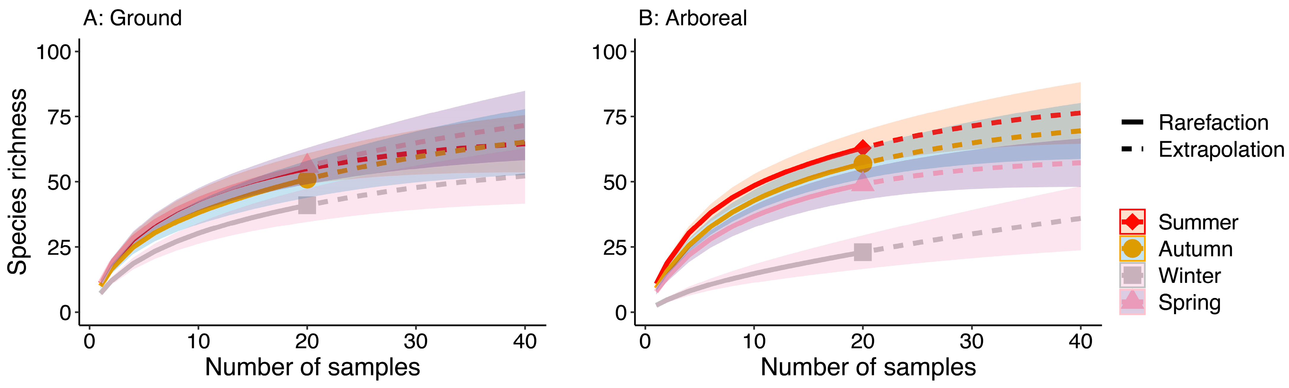
3.2. Gamma Diversity and Sampling Sufficiency

Species accumulation curves showed that the total number of ant species (gamma diversity) was highest at the lowest elevational band (300 m a.s.l.) and progressively declined with increasing elevation (Figure S1). In the ground samples, the gamma diversity was not significantly different between 300 and 500 m bands and between 700 and 900 m bands with 95% confidence intervals overlapping (Figure S1A). In the arboreal samples, gamma diversity was not significantly different among 300, 500, and 700 m bands (Figure S1B). In contrast to elevational differences, seasonal differences were not as clearly discernible (Figure 1). Gamma diversity was highest in austral summer (January), followed by autumn (March), spring (October), and winter (July), but summer, autumn, and spring gamma diversity were not significantly different (Figure 1). Sample coverage achieved over 80% for both ground- and arboreal-foraging ants across elevational bands (Figure S2) and across seasons (Figure S3), except for arboreal-foraging ants collected in July due to sporadic occurrences of ant species in this austral winter (Figure S2).

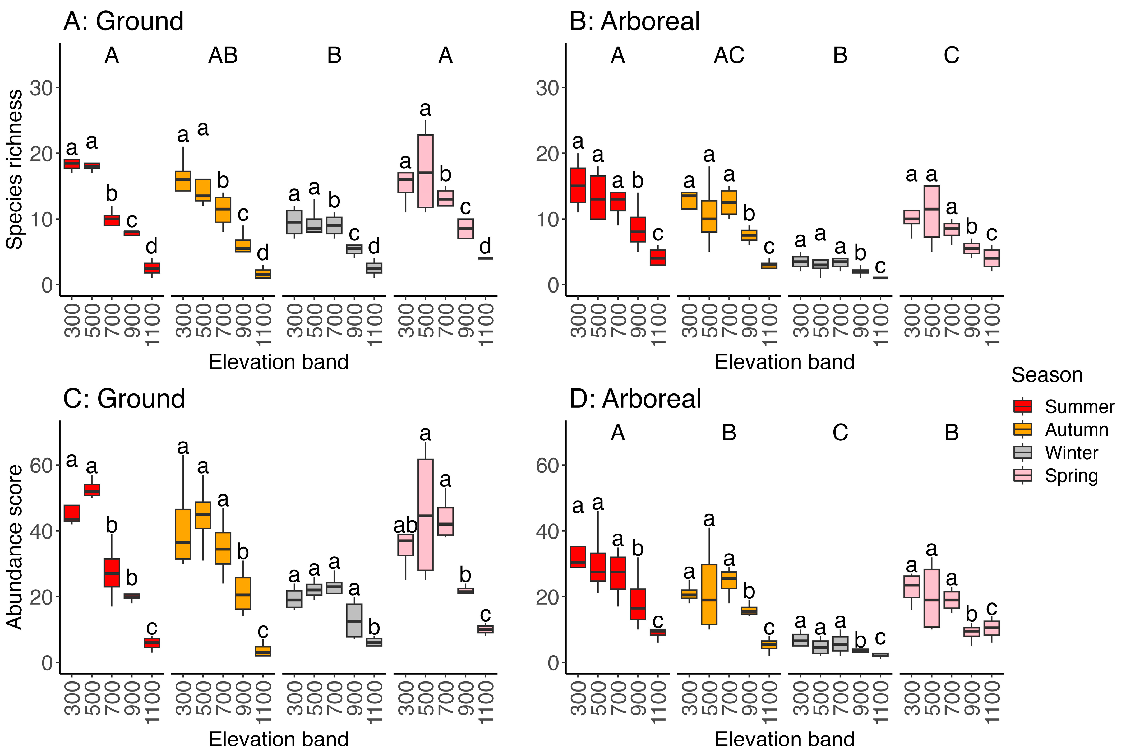
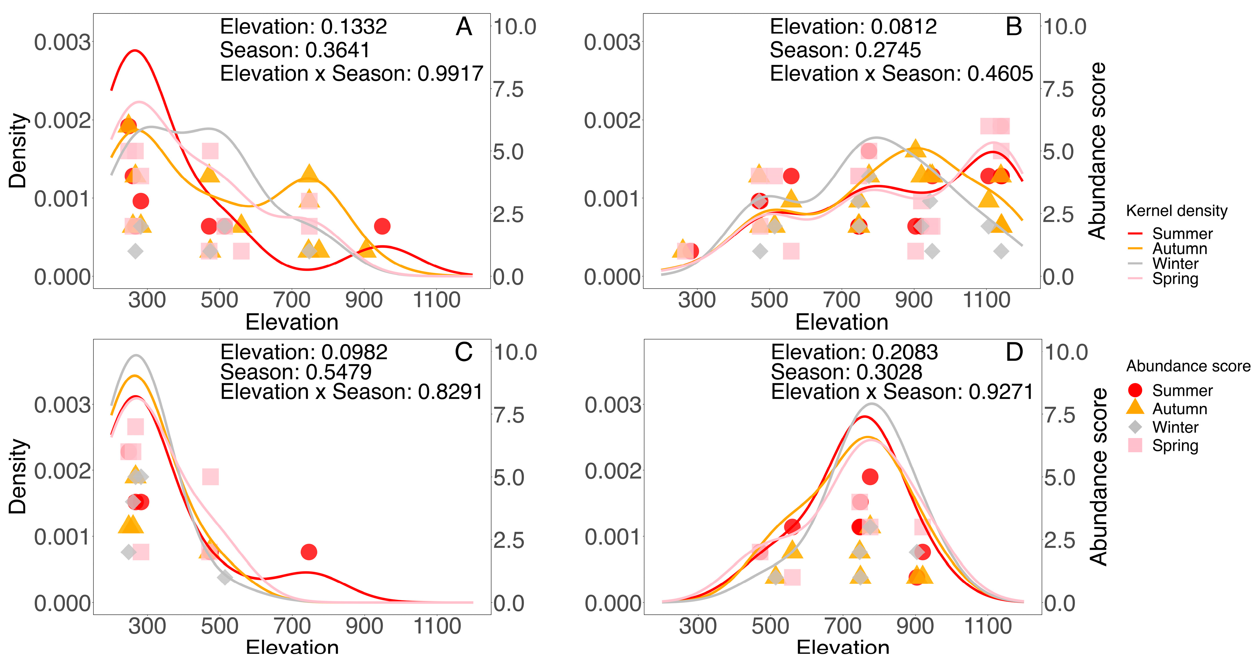
3.3. Species Richness (Alpha Diversity) and Abundance Scores

Both elevation and season significantly influenced the species richness and total abundance score of ground and arboreal ants (Table 1). However, the interaction between elevation and season was significant only for the abundance score of the ground active ants. Ant species richness declined with increasing elevation across all seasons (Figure 2A,B). Significant differences in ground ant richness among all elevational bands except 300 and 500 m were observed (Figure 2A). Similarly, arboreal ants showed the highest richness at 300, 500, and 700 m, then progressively declined at 900 and 1100 m a.s.l. (Figure 2B). The abundance scores of ground ants were the lowest at 1100 m a.s.l. but showed variable elevational patterns across seasons in the lower elevations (i.e., interaction effect; Figure 2C). For arboreal ants, elevational patterns in abundance scores did not vary with season and showed no significant differences across 300, 500, and 700 m but declined at 900 and 1100 m a.s.l. (Figure 2D).

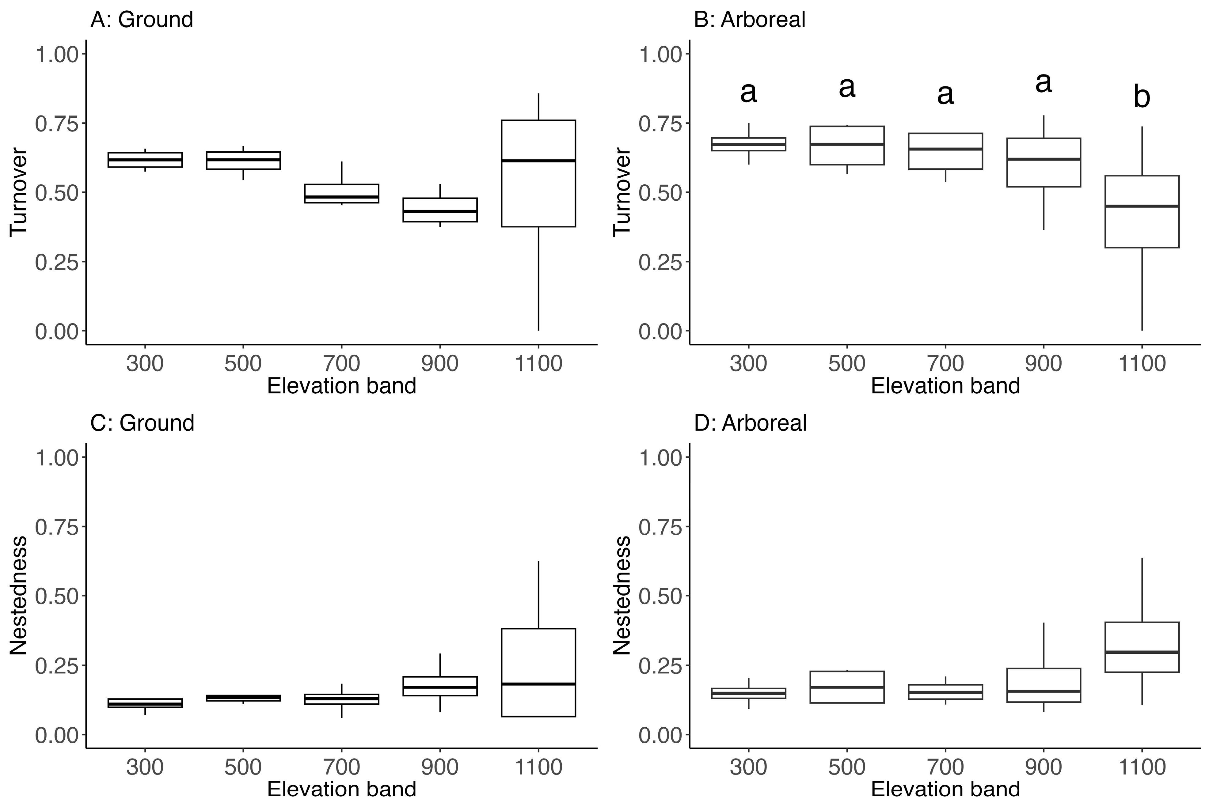
3.4. Beta Turnover and Nestedness

For both ground and arboreal ants, beta turnover decreased while beta nestedness increased with elevation (Figure 3). However, the results of GLMMs showed that elevation was only significant for arboreal ant turnover (Table S1), with only the 1100 m band being significantly lower than others (Figure 3B).

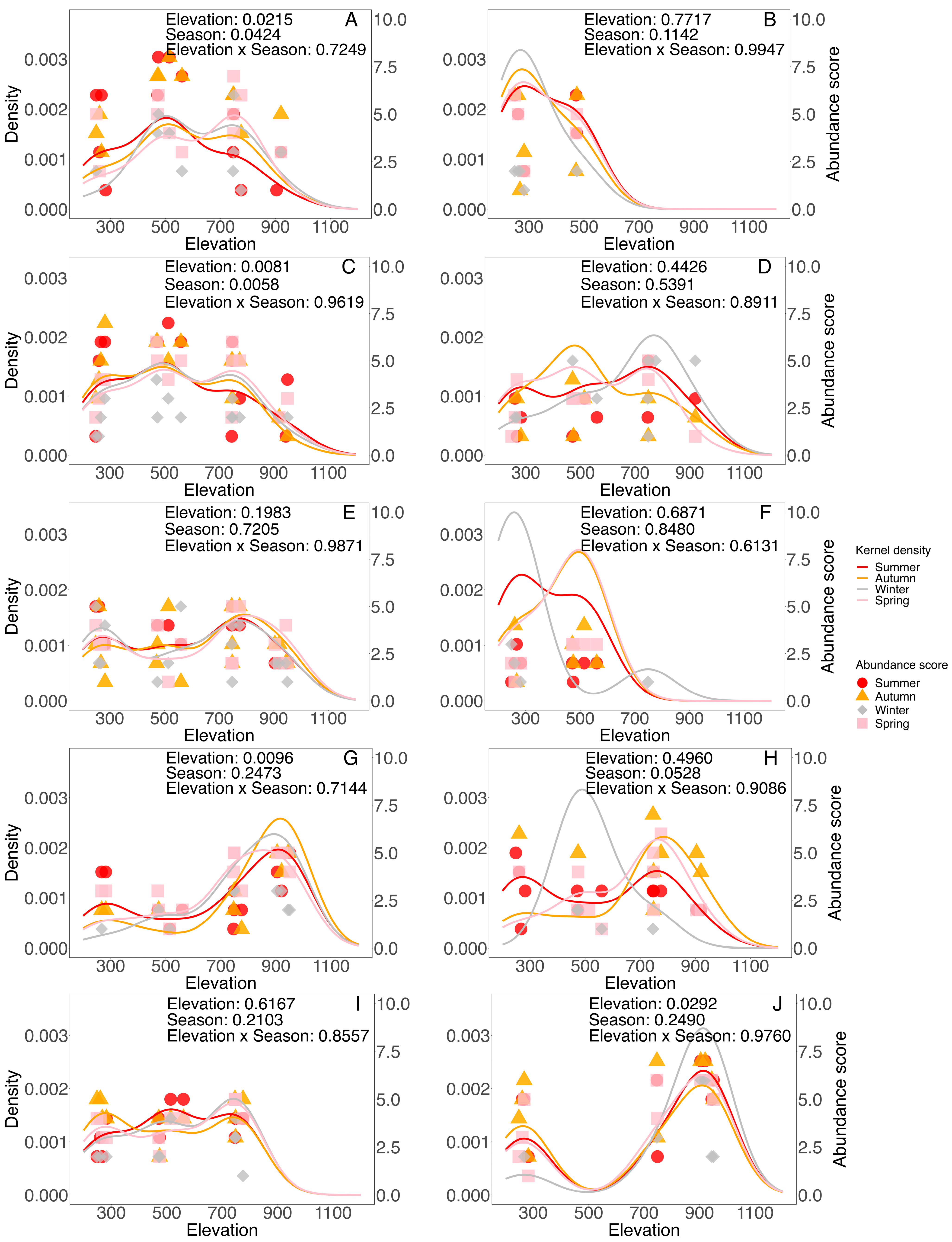
3.5. Individual Ant Species

The GLMM analysis of individual ant species showed significant effects of elevation on the abundance scores of some ant species (Table S2; see also insets in Figure 4 and Figure 5). Two commonly collected ant species, Carebara BATH1 (Figure 4A) and Hypoponera BATH2 (Figure 4C), showed strong affiliations towards lower elevational bands (300–900 m), whereas Pheidole BATH1 was more commonly collected at mid-elevation (700 and 900 m) (Figure 4G). Solenopsis BATH1 showed bimodal distribution at low (300 m) and mid-elevations (700 and 900 m) (Figure 4J). Season had significant effects on the abundance scores of only Carebara BATH1 and Hypoponera BATH2 (Figure 4A,C), but they remained strongly affiliated with lower elevations.

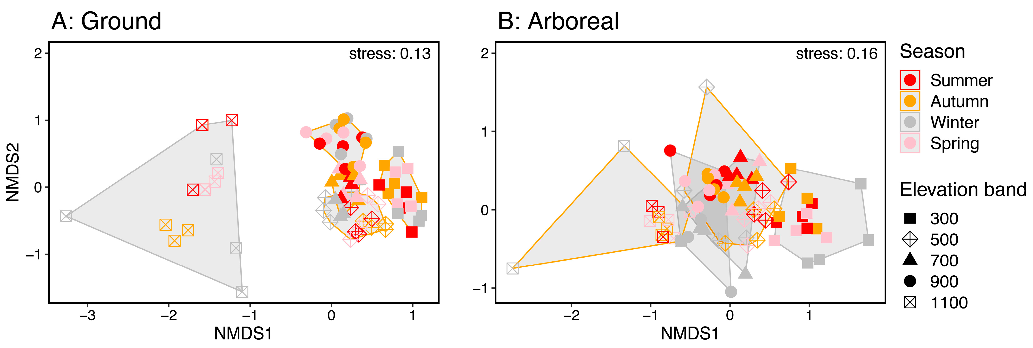
3.6. Species Composition

Ground ants showed progressive changes in community composition from 300 to 900 m elevational bands, but ant communities at 1100 m were substantially different from other elevations (Figure 6A). Arboreal ants also showed progressive changes across the elevations, but some plots at mid-elevations (500–900 m) were similar and showed overlapping patterns on the ordination (Figure 6B). The PERMANOVA confirmed the significant effects of elevation on both ground and arboreal ant community composition (Table 2). The results also showed significant effects of season and the interaction between elevation and season (Table 2). Despite the significant effects of season, all ant communities showed similar composition within each elevational band (Figure S4). Procrustes analyses showed significant correlations between any pairs of seasons in both ground and arboreal ant communities, suggesting similar elevational patterns across the seasons (Table S3).

3.7. Indicator Species

The indicator value protocol identified only two arboreal species as indicators for certain seasons (Table S5). None of the ground species were identified as indicators for any season. For elevation, a total of 43 species (27 ground and 22 arboreal species) were identified as indicators for specific elevational bands (or a range of successive elevational bands). Among these, six were found to be indicative of the same elevational band for both ground and arboreal strata (Chelaner BATH3 for 700 m; Monomorium BATH2 for 1100 m; Notoncus capitatus, Pheidole BATH6, and Pheidole BATH4 for 300–500 m; and Rhytidoponera victoriae for 300–700 m). All indicator species identified were strong indicators (i.e., indicator value > 0.7).

4. Discussion

Elevational diversity patterns have been well researched for various taxa and from many different locations, yet the importance of temporal (e.g., seasonality) and spatial dynamics (e.g., microhabitat use) has been largely overlooked. In this study, we conducted intensive ant sampling and investigated elevational diversity patterns between two different strata (ground vs. arboreal) across four seasons along the same elevational transect. These results expanded on a previous study [37] and incorporated vertical strata and seasonal samples into the analyses. Our sampling demonstrated high sampling efficiency, achieving 80% coverage for all seasons except winter, when ant activity was limited. During winter, we observed a reduced number of ant species and individuals, which were collected sporadically. Despite the seasonal fluctuations in ant activity, our results highlight a general decline in ant species richness and abundance scores and progressive changes in ant community compositions with increasing elevation. More importantly, we found that the elevational patterns were similar between ground and arboreal ants and remained consistent across the four seasons.
The elevational decline in species richness has also been observed in earlier studies from the study region [37,60] and elsewhere [23,61,62]. Theoretical predictions suggest that the mid-elevation peak in species richness is the most common pattern [21,63], and this too has been previously documented for ants [22,64]. Despite using ants from only litter extraction and bark spray samples, we showed consistent elevational declines in ant diversity across seasons for both ground and arboreal ants. However, a mid-elevation peak still might have emerged if samples from lower elevations were available. Regrettably, lower elevation sites were available only in small rainforest remnants, wherein assemblages may not be comparable to those of the continuous rainforest used in the study [37].
Our findings regarding seasonal ant distributions along elevational gradients differ from the uphill and downhill seasonal shifts reported for many tropical lepidopteran groups [26]. They hypothesized that these shifts are caused by seasonality in weather and resource availability, leading to delays in adult emergence and adult migration, respectively. Another study on tropical ants found size and position changes in the mid-elevation peak depending on the season [22]. They showed that more intense seasonal fluctuations in temperature at lower elevations allowed for greater variation in ant richness, which resulted in the seasonal peak changes. In contrast, we found that ant diversity did not change their elevational patterns seasonally. Although seasonal nest relocation is practiced by many ant species [65], the distances moved during relocation may not be long enough to affect their elevational distributions. Instead, seasonal influence affects only their activity levels, as reflected by lower ant numbers during winter rather than their spatial distribution.
For both ground and arboreal ant beta diversity, seasonal turnover was greater than nestedness across all elevations. It is important to note that some species may remain present but undetected during cooler seasons due to reduced activity. Thus, seasonal turnover patterns may partly reflect detection biases associated with surface-based sampling. The observed richness from our sampling showed that species composition changes across seasons, with different ant species replacing one another rather than simply being subsets of the same community. This would predict distinct sets of indicator species across seasons. However, we did not find many indicator species for the individual (or combinations of) seasons. Furthermore, when analyzing individual species, we found that both ground and arboreal ants exhibited consistent elevational patterns across seasons. These indicate that seasonal effects influence community structure more strongly than the distributions of individual species. As our analysis was limited to common ant species, turnover may operate more strongly on rarer species. Interestingly, we found decreasing turnover and increasing nestedness with elevation, especially for arboreal ant communities. This may be due to the harsh environmental conditions in arboreal habitats that work as environmental filters across the seasons, causing certain species to disappear in the winter [66].
We predicted that arboreal ants are less sensitive to elevational differences than ground ants. However, we found that ground and arboreal ant communities exhibited similar patterns along the elevational gradient of the subtropical rainforest. Similarly, a study on Middle American wet forest ants found similar overall patterns in ground and arboreal ants [64]. A potential explanation is that the arboreal sampling (sweeping and vegetation beating used by Longino et al. [64] and bark spraying in this study) was limited to within 3 m aboveground. Although ants sampled from this height can be classified as arboreal species, they may also include ground-foraging arboreal species and canopy-foraging ground species [67] that may have been sampled in both the ground and arboreal strata. In fact, 44 of the 80 ground and 88 arboreal species were shared between strata. Our methods presumably missed canopy-dwelling ants that inhabit tree holes, epiphytes, or arboreal soil [68]. These upper canopy taxa could exhibit different elevational patterns compared to the arboreal species sampled in this study, potentially affecting the observed differences between ground and arboreal ant communities [32].
Our study demonstrates how ants can serve as valuable indicators of climate change, as their strong elevational distribution patterns have been observed across studies worldwide [21]. Unlike other taxa that exhibit seasonal shifts in response to short-term environmental fluctuations, ants appear to be less affected by intra-annual seasonal changes. This stability suggests that their distributions reflect long-term climatic trends rather than temporary seasonal variations [69]. As a result, ants may serve as effective bioindicators for monitoring the long-term impacts of climate change on biodiversity.

5. Conclusions

Ant diversity declined consistently with increasing elevation across both ground and arboreal strata and remained stable across seasons, highlighting the robustness of elevational patterns despite seasonal variation in activity levels. Unlike other insect taxa that show seasonal upslope or downslope shifts, ants exhibited consistent elevational distributions throughout the year, suggesting their sensitivity to long-term environmental gradients rather than short-term climatic fluctuations. Beta diversity patterns showed that seasonal turnover dominated over nestedness at all elevations, though high-elevation sites—especially for arboreal ants—exhibited increased nestedness, likely due to harsher environmental filtering. Interestingly, ground and arboreal ant communities responded similarly to elevational gradients, possibly due to the overlap in foraging height and limitations in canopy sampling. These findings underscore the value of ants as bioindicators for long-term climate monitoring. By integrating spatial (vertical stratification) and temporal (seasonal) perspectives, this study contributes novel insights into how insect communities, particularly ants, respond to elevational and seasonal dynamics in subtropical rainforests. Given their ecological sensitivity and predictability, monitoring ant communities along elevation gradients may provide an effective and early-warning system for assessing the impacts of climate change and informing biodiversity conservation strategies.

Supplementary Materials

The following supporting information can be downloaded at: https://www.mdpi.com/article/10.3390/f16040664/s1, Figure S1: Sample-based species accumulation curves of the ground ants and arboreal ants; Figure S2: Sample-based sample coverage curves of the ground ants and arboreal ants collected from different elevational bands; Figure S3: Sample-based sample coverage curves of the ground ants and arboreal ants collected from different seasons; Figure S4: NMDS ordination of ground and arboreal ant communities collected from different elevational bands and seasons; Table S1: Summary result of the generalized linear mixed models on beta turnover and nestedness components of ant communities collected from ground and arboreal habitats; Table S2: Summary result of the generalized linear mixed models on the abundance scores of individual ground and arboreal species; Table S3: Summary result of the Procrustes analysis on the ground and arboreal ant communities; Table S4: Significant ground and arboreal indicator ant species for the different elevational bands across the four seasons; Table S5: Significant indicator arboreal ant species for the different seasons across the five elevational bands; Table S6: List of ant species across seasons and elevations from both ground and arboreal habitats.

Author Contributions

Conceptualization, C.J.B., L.A.A., R.L.K., M.C. and A.N.; methodology, C.J.B., L.A.A., R.L.K., M.C. and A.N.; validation, C.J.B. and A.N.; formal analysis, P.K., L.P., M.J.M.A. and A.N.; investigation, C.J.B., L.A.A., R.L.K., M.C. and A.N.; resources, C.J.B., R.L.K. and M.C.; data curation, C.J.B. and A.N.; writing—original draft preparation, P.K., M.J.M.A. and A.N.; writing—review and editing, P.K., B.D.B., M.J.M.A. and A.N.; visualization, P.K., L.P., M.J.M.A. and A.N.; supervision, A.N.; project administration, C.J.B., R.L.K., M.C. and A.N.; funding acquisition, R.L.K., M.C. and A.N. All authors have read and agreed to the published version of the manuscript.

Funding

This research was funded by the Queensland–Chinese Academy of Sciences Biotechnology Fund, grant number GJHZ1130, Queensland Government Smart State Grant, Griffith University, Queensland Museum, Queensland Herbarium, SEQ Catchments Network, and the Global Canopy Programme. A.N. was funded by the National Natural Science Foundation of China International (Regional) Cooperation and Exchange Project, grant number 32161160324, and the 14th Five-Year Plan of Xishuangbanna Tropical Botanical Garden, Chinese Academy of Sciences, grant number E3ZKFF1K.

Data Availability Statement

The data presented in this study are available upon request from the corresponding author.

Acknowledgments

We thank David Putland, Heather Christensen, and all other IBISCA Queensland support staff and volunteers for their assistance during the project. Susan Wright, Geoff Thompson, and Anna Marcora (Queensland Museum) are thanked for conducting ant sampling. Other IBISCA Queensland participants, particularly Geoff Monteith, Christine Lambkin, Kyran Staunton, Frode Ødegaard, Juergen Scmidl, and Torsten Bitner provided access to the ants from their sampling programs.

Conflicts of Interest

The authors declare no conflicts of interest. The funders had no role in the design of the study; in the collection, analyses, or interpretation of data; in the writing of the manuscript; or in the decision to publish the results.

Appendix A

Table A1. List of ant species collected across arboreal and ground habitats. A check mark (✓) indicates presence; a cross (✗) indicates absence.
Species NumberSpecies NameArborealGround
1Amblyopone australis Erichson, 1842
2Anonychomyrma QM3
3Anonychomyrma QM9
4Arnoldius QM2
5Camponotus BATH1
6Camponotus BATH2
7Camponotus froggatti Forel, 1902
8Carebara BATH1
9Carebara BATH2
10Chelaner BATH3
11 Chelaner BATH4
12Chelaner BATH6
13Chelaner kiliani (Forel, 1902)
14Chelaner nigriceps (Heterick, 2001)
15Chelaner tambourinensis (Forel, 1915)
16Colobopsis BATH3
17Colobopsis BATH4
18Colobostruma biconvexa Shattuck, 2000
19Colobostruma froggatti (Forel, 1913)
20Crematogaster BATH1
21Crematogaster BATH3
22Cryptopone BATH1
23Cryptopone BATH2
24Discothyrea BATH1
25Discothyrea BATH2
26Discothyrea BATH3
27Discothyrea BATH4
28Eurhopalothrix australis Brown & Kempf, 1960
29Heteroponera BATH1
30Heteroponera BATH2
31Hypoponera BATH1
32Hypoponera BATH2
33Hypoponera BATH3
34Hypoponera BATH5
35Hypoponera BATH6
36Hypoponera BATH7
37Leptogenys BATH1
38Leptogenys mjobergi Forel, 1915
39Leptogenys sjostedti Forel, 1915
40Leptomyrmex burwelli Smith, D.J. & Shattuck, 2009
41Leptomyrmex cnemidatus Wheeler, W.M., 1915
42Leptomyrmex tibialis Emery, 1895
43Lioponera BATH1
44Lioponera BATH2
45Lioponera BATH3
46Lordomyrma BATH1
47Mayriella abstinens Forel, 1902
48Mayriella overbecki Viehmeyer, 1925
49Mayriella spinosior Wheeler, W.M., 1935
50Mesoponera australis (Forel, 1900)
51Monomorium BATH2
52Monomorium BATH5
53Monomorium BATH7
54Myrmecia brevinoda Forel, 1910
55Myrmecia nigrocincta Smith, F., 1858
56Myrmecina australis Wheeler, G.C. & Wheeler, J., 1973
57Myrmecorhynchus carteri Clark, 1934
58Myrmecorhynchus emeryi André, 1896
59Notoncus capitatus Forel, 1915
60Notoncus spinisquamis (André, 1896)
61Notostigma foreli Emery, 1920
62Nylanderia QM1
63Ochetellus BATH2
64Orectognathus antennatus Smith, F., 1853
65Orectognathus elegantulus Taylor, 1977
66Orectognathus phyllobates Brown, 1958
67Orectognathus robustus Taylor, 1977
68Orectognathus rostratus Lowery, 1967
69Orectognathus versicolor Donisthorpe, 1940
70Paraparatrechina QM4
71Paraparatrechina QM8
72Pheidole BATH1
73Pheidole BATH2
74Pheidole BATH3
75Pheidole BATH4
76Pheidole BATH5
77Pheidole BATH6
78Pheidole BATH7
79Pheidole BATH10
80Pheidole BATH11
81Pheidole dispar (Forel, 1895)
82Plagiolepis QM2
83Platythyrea parallela (Smith, F., 1859)
84Podomyrma BATH1
85Podomyrma BATH2
86Podomyrma BATH3
87Podomyrma BATH6
88Podomyrma BATH7
89Podomyrma BATH8
90Polyrhachis BATH1
91Polyrhachis clio Forel, 1902
92Polyrhachis maculata Forel, 1915
93Polyrhachis ornata Mayr, 1876
94Polyrhachis pilosa Donisthorpe, 1938
95Ponera leae Forel, 1913
96Prionopelta robynmae Shattuck, 2008
97Pristomyrmex wheeleri Taylor, 1965
98Probolomyrmex greavesi Taylor, 1965
99Prolasius QM1
100Prolasius QM2
101Prolasius QM4
102Prolasius QM6
103Prolasius QM7
104Prolasius QM8
105Prolasius QM9
106Pseudoneoponera BATH1
107Rhopalomastix BATH1
108Rhopalothrix orbis Taylor, 1968
109Rhytidoponera chalybaea Emery, 1901
110Rhytidoponera croesus Emery, 1901
111Rhytidoponera victoriae (André, 1896)
112Solenopsis BATH1
113Stigmacros major McAreavey, 1957
114Stigmacros QM22
115Stigmatomma QM1
116Strumigenys deuteras Bolton, 2000
117Strumigenys harpyia Bolton, 2000
118Strumigenys perplexa (Smith, F., 1876)
119Tapinoma QM2
120Tapinoma QM3
121Tapinoma QM4
122Tapinoma QM6
123Technomyrmex jocosus Forel, 1910
124Zasphinctus BATH1

References

  1. Rosenzweig, M.L. Species Diversity in Space and Time; Cambridge University Press: Cambridge, UK, 1995. [Google Scholar]
  2. Magurran, A.E. Species abundance distributions over time. Ecol. Lett. 2007, 10, 347–354. [Google Scholar] [CrossRef]
  3. Willig, M.R.; Presley, S.J. Latitudinal gradients of biodiversity. In Reference Module in Life Sciences; Elsevier Inc.: Amsterdam, The Netherlands, 2017; pp. 1–17. [Google Scholar]
  4. Mannion, P.D.; Upchurch, P.; Benson, R.B.J.; Goswami, A. The latitudinal biodiversity gradient through deep time. Trends Ecol. Evol. 2014, 29, 42–50. [Google Scholar] [CrossRef] [PubMed]
  5. Willig, M.R.; Kaufman, D.M.; Stevens, R.D. Latitudinal gradients of biodiversity: Pattern, process, scale, and synthesis. Annu. Rev. Ecol. Evol. Syst. 2003, 34, 273–309. [Google Scholar] [CrossRef]
  6. Lundholm, J.T. Plant species diversity and environmental heterogeneity: Spatial scale and competing hypotheses. J. Veg. Sci. 2009, 20, 377–391. [Google Scholar] [CrossRef]
  7. Körner, C. The use of “altitude” in ecological research. Trends Ecol. Evol. 2007, 22, 569–574. [Google Scholar] [CrossRef]
  8. Sanders, N.J.; Rahbek, C. The patterns and causes of elevational diversity gradients. Ecography 2012, 35, 1–3. [Google Scholar] [CrossRef]
  9. Barry, R.G. Mountain Weather and Climate; Routledge: Abingdon, UK, 2013. [Google Scholar]
  10. Zhang, L.; Hay, W.W.; Wang, C.; Gu, X. The evolution of latitudinal temperature gradients from the latest cretaceous through the present. Earth-Sci. Rev. 2019, 189, 147–158. [Google Scholar] [CrossRef]
  11. Sundqvist, M.K.; Sanders, N.J.; Wardle, D.A. Community and ecosystem responses to elevational gradients: Processes, mechanisms, and insights for global change. Annu. Rev. Ecol. Evol. Syst. 2013, 44, 261–280. [Google Scholar] [CrossRef]
  12. Rahbek, C. The elevational gradient of species richness: A uniform pattern? Ecography 1995, 18, 200–205. [Google Scholar] [CrossRef]
  13. Kessler, M.; Kluge, J.; Hemp, A.; Ohlemüller, R. A global comparative analysis of elevational species richness patterns of ferns. Glob. Ecol. Biogeogr. 2011, 20, 868–880. [Google Scholar] [CrossRef]
  14. Sanders, N.J. Elevational gradients in ant species richness: Area, geometry, and Rapoport’s rule. Ecography 2002, 25, 25–32. [Google Scholar] [CrossRef]
  15. McCain, C.M.; Grytnes, J. Elevational gradients in species richness. In Encyclopedia of Life Sciences; Wiley: Hoboken, NJ, USA, 2010. [Google Scholar] [CrossRef]
  16. Dehling, D.M.; Töpfer, T.; Schaefer, H.M.; Jordano, P.; Böhning-Gaese, K.; Schleuning, M. Functional relationships beyond species richness patterns: Trait matching in plant-bird mutualisms across scales. Glob. Ecol. Biogeogr. 2014, 23, 1085–1093. [Google Scholar] [CrossRef]
  17. Stark, J.; Lehman, R.; Crawford, L.; Enquist, B.J.; Blonder, B. Does environmental heterogeneity drive functional trait variation? A test in montane and alpine meadows. Oikos 2017, 126, 1650–1659. [Google Scholar] [CrossRef]
  18. Rahbek, C. The Role of spatial scale and the perception of large-scale species-richness patterns. Ecol. Lett. 2005, 8, 224–239. [Google Scholar] [CrossRef]
  19. Brehm, G.; Colwell, R.K.; Kluge, J. The role of environment and mid-domain effect on moth species richness along a tropical elevational gradient. Glob. Ecol. Biogeogr. 2007, 16, 205–219. [Google Scholar] [CrossRef]
  20. Sanders, N.J.; Moss, J.; Wagner, D. Patterns of ant species richness along elevational gradients in an arid ecosystem. Glob. Ecol. Biogeogr. 2003, 12, 93–102. [Google Scholar] [CrossRef]
  21. Szewczyk, T.; McCain, C.M. A systematic review of global drivers of ant elevational diversity. PLoS ONE 2016, 11, e0155404. [Google Scholar] [CrossRef]
  22. Bishop, T.R.; Robertson, M.P.; van Rensburg, B.J.; Parr, C.L. Elevation–diversity patterns through space and time: Ant communities of the Maloti-Drakensberg Mountains of southern Africa. J. Biogeogr. 2014, 41, 2256–2268. [Google Scholar] [CrossRef]
  23. Marathe, A.; Priyadarsanan, D.R.; Krishnaswamy, J.; Shanker, K. Spatial and climatic variables independently drive elevational gradients in ant species richness in the eastern Himalaya. PLoS ONE 2020, 15, e0227628. [Google Scholar] [CrossRef]
  24. Sanders, N.J.; Lessard, J.; Fitzpatrick, M.C.; Dunn, R.R. Temperature, but not productivity or geometry, predicts elevational diversity gradients in ants across spatial grains. Glob. Ecol. Biogeogr. 2007, 16, 640–649. [Google Scholar] [CrossRef]
  25. Schebeck, M.; Lehmann, P.; Laparie, M.; Bentz, B.J.; Ragland, G.J.; Battisti, A.; Hahn, D.A. Seasonality of forest insects: Why diapause matters. Trends Ecol. Evol. 2024, 39, 757–770. [Google Scholar] [CrossRef] [PubMed]
  26. Maicher, V.; Sáfián, S.; Murkwe, M.; Delabye, S.; Przybyłowicz, Ł.; Potocký, P.; Kobe, I.N.; Janeček, Š.; Mertens, J.E.J.; Fokam, E.B.; et al. Seasonal shifts of biodiversity patterns and species’ elevation ranges of butterflies and moths along a complete rainforest elevational gradient on Mount Cameroon. J. Biogeogr. 2020, 47, 342–354. [Google Scholar] [CrossRef]
  27. Kishimoto-Yamada, K.; Itioka, T. How much have we learned about seasonality in tropical insect abundance since Wolda (1988)? Entomol. Sci. 2015, 18, 407–419. [Google Scholar] [CrossRef]
  28. Araújo, C.d.O.; Hortal, J.; de Macedo, M.V.; Monteiro, R.F. Elevational and seasonal distribution of scarabaeinae dung beetles (Scarabaeidae: Coleoptera) at Itatiaia National Park (Brazil). Int. J. Trop. Insect Sci. 2022, 42, 1579–1592. [Google Scholar] [CrossRef]
  29. Kaspari, M.; Donnell, S.; Kercher, J.R. Energy, density, and constraints to species richness: Ant assemblages along a productivity gradient. Am. Nat. 2000, 155, 280–293. [Google Scholar] [CrossRef]
  30. Scheffers, B.R.; Phillips, B.L.; Laurance, W.F.; Sodhi, N.S.; Diesmos, A.; Williams, S.E. Increasing arboreality with altitude: A novel biogeographic dimension. Proc. R. Soc. B Biol. Sci. 2013, 280, 20131581. [Google Scholar] [CrossRef]
  31. Leahy, L.; Scheffers, B.R.; Andersen, A.N.; Hirsch, B.T.; Williams, S.E. Vertical niche and elevation range size in tropical ants: Implications for climate resilience. Divers. Distrib. 2021, 27, 485–496. [Google Scholar] [CrossRef]
  32. Leahy, L.; Scheffers, B.R.; Andersen, A.N.; Williams, S.E. Rates of species turnover across elevation vary with vertical stratum in rainforest ant assemblages. Ecography 2024, 2024, e06972. [Google Scholar] [CrossRef]
  33. Nakamura, A.; Kitching, R.L.; Cao, M.; Creedy, T.J.; Fayle, T.M.; Freiberg, M.; Hewitt, C.N.; Itioka, T.; Koh, L.P.; Ma, K.; et al. Forests and their canopies: Achievements and horizons in canopy science. Trends Ecol. Evol. 2017, 32, 438–451. [Google Scholar] [CrossRef]
  34. Oliveira, B.F.; Scheffers, B.R. Vertical stratification influences global patterns of biodiversity. Ecography 2019, 42, 249. [Google Scholar] [CrossRef]
  35. Arruda, F.V.; Camarota, F.; Ramalho, W.P.; Izzo, T.J.; Santos Almeida, R.P. Seasonal variation of ground and arboreal ants in forest fragments in the highly-threatened Cerrado-Amazon transition. J. Insect Conserv. 2021, 25, 897–904. [Google Scholar] [CrossRef]
  36. Basset, Y.; Cizek, L.; Cuénoud, P.; Didham, R.K.; Novotny, V.; Ødegaard, F.; Roslin, T.; Tishechkin, A.K.; Schmidl, J.; Winchester, N.N.; et al. Arthropod distribution in a tropical rainforest: Tackling a four dimensional puzzle. PLoS ONE 2015, 10, e0144110. [Google Scholar] [CrossRef]
  37. Burwell, C.J.; Nakamura, A. Distribution of ant species along an altitudinal transect in continuous rainforest in subtropical Queensland, Australia. Mem. Queensl. Mus. 2011, 55, 403–411. [Google Scholar]
  38. Kitching, R.L.; Putland, D.; Ashton, L.A.; Laidlaw, M.J.; Boulter, S.L.; Christensen, H.; Lambkin, C.L. Detecting biodiversity changes along climatic gradients: The IBISCA-Queensland project. Mem. Queensl. Mus. 2011, 55, 235–250. [Google Scholar]
  39. Laidlaw, M.J.; McDonald, W.J.F.; Hunter, R.J.; Kitching, R.L. Subtropical rainforest turnover along an altitudinal gradient. Mem. Queensl. Mus. 2011, 55, 271–290. [Google Scholar]
  40. Strong, C.L.; Boulter, S.L.; Laidlaw, M.J.; Maunsell, S.C.; Putland, D.; Kitching, R.L. The physical environment of an altitudinal gradient in the rainforest of Lamington National Park, Southeast Queensland. Mem. Queensl. Mus. 2011, 55, 251–270. [Google Scholar]
  41. Northcote, K.H. A Factual Key for the Recognition of Australian Soils; Rellium Technical Publications: Glenside, Australia, 1979. [Google Scholar]
  42. FAO. World Reference Base for Soil Resources; Food and Agriculture Organization of the United Nations: Rome, Italy, 1998. [Google Scholar]
  43. Bolton, B. Synopsis and classification of Formicidae. Mem. Am. Entomol. Inst. 2003, 71, 1–370. [Google Scholar]
  44. Shattuck, S.; Barnett, N. Australian Ants Online: The Guide to Australian Ant Fauna. 2001. Available online: http://www.ento.csiro.au/science/ants/ (accessed on 29 October 2007).
  45. Hoffmann, B.D.; Kay, A. Pisonia grandis monocultures limit the spread of an invasive ant—A case of carbohydrate quality? Biol. Invasions 2009, 11, 1403–1410. [Google Scholar] [CrossRef]
  46. R Core Team. R: A Language and Environment for Statistical Computing; R Foundation for Statistical Computing: Vienna, Austria, 2022; Available online: https://www.R-project.org/ (accessed on 25 March 2025).
  47. Wickham, H. ggplot2: Elegant Graphics for Data Analysis; Springer: New York, NY, USA, 2016. [Google Scholar]
  48. Hsieh, T.C.; Ma, K.H.; Chao, A. iNEXT: An R package for rarefaction and extrapolation of species diversity (Hill numbers). Methods Ecol. Evol. 2016, 7, 1451–1456. [Google Scholar] [CrossRef]
  49. Chao, A.; Gotelli, N.J.; Hsieh, T.C.; Sander, E.L.; Ma, K.H.; Colwell, R.K.; Ellison, A.M. Rarefaction and extrapolation with Hill numbers: A framework for sampling and estimation in species diversity studies. Ecol. Monogr. 2014, 84, 45–67. [Google Scholar] [CrossRef]
  50. Brooks, M.E.; Kristensen, K.; van Benthem, K.J.; Magnusson, A.; Berg, C.W.; Nielsen, A.; Skaug, H.J.; Mächler, M.; Bolker, B.M. glmmTMB balances speed and flexibility among packages for zero-inflated generalized linear mixed modeling. R J. 2017, 9, 378–400. [Google Scholar] [CrossRef]
  51. Lüdecke, D.; Ben-Shachar, M.S.; Patil, I.; Waggoner, P.; Makowski, D. performance: An R package for assessment, comparison and testing of statistical models. J. Open Source Softw. 2021, 6, 3139. [Google Scholar] [CrossRef]
  52. Fox, J.; Weisberg, S. Using Car and Effects Functions in Other Functions. 2020. Available online: http://download.nust.na/pub3/cran/web/packages/car/vignettes/embedding.pdf (accessed on 25 March 2025).
  53. Lenth, R. Emmeans: Estimated Marginal Means, Aka Least-Squares Means. R Package Version 1.10.2. 2024. Available online: https://CRAN.R-project.org/package=emmeans (accessed on 25 March 2025).
  54. Baselga, A.; Orme, D.; Villéger, S.; De Bortoli, J.; Leprieur, F.; Logez, M. Betapart: Partitioning Beta Diversity into Turnover and Nestedness Components. R Package Version 1.5.6. 2022. Available online: https://cran.r-project.org/web/packages/betapart/index.html (accessed on 25 March 2025).
  55. Baselga, A.; Orme, C.D.L. Betapart: An R package for the study of beta diversity. Methods Ecol. Evol. 2012, 3, 808–812. [Google Scholar] [CrossRef]
  56. Oksanen, J.; Simpson, G.; Blanchet, F.; Kindt, R.; Legendre, P.; Minchin, P.; O’Hara, R.; Solymos, P.; Stevens, M.; Szoecs, E.; et al. Vegan: Community Ecology Package; R Package Version 2.6-4. 2022. Available online: https://CRAN.R-project.org/package=vegan (accessed on 25 March 2025).
  57. Dufrene, M.; Legendre, P. Species assemblages and indicator species: The need for a flexible asymmetrical approach. Ecol. Monogr. 1997, 67, 345–366. [Google Scholar] [CrossRef]
  58. McGeoch, M.A.; Van Rensburg, B.J.; Botes, A. The verification and application of bioindicators: A case study of dung beetles in a savanna ecosystem. J. Appl. Ecol. 2002, 39, 661–672. [Google Scholar] [CrossRef]
  59. De Cáceres, M.; Legendre, P. Associations between species and groups of sites: Indices and statistical inference. Ecology 2009, 90, 3566–3574. [Google Scholar] [CrossRef] [PubMed]
  60. Burwell, C.J.; Nakamura, A. Can changes in ant diversity along elevational gradients in tropical and subtropical Australian rainforests be used to detect a signal of past lowland biotic attrition? Austral Ecol. 2016, 41, 209–218. [Google Scholar] [CrossRef]
  61. Liu, C.; Dudley, K.L.; Xu, Z.; Economo, E.P. Mountain metacommunities: Climate and spatial connectivity shape ant diversity in a complex landscape. Ecography 2018, 41, 101–112. [Google Scholar] [CrossRef]
  62. Fontanilla, A.M.; Nakamura, A.; Xu, Z.; Cao, M.; Kitching, R.L.; Tang, Y.; Burwell, C.J. Taxonomic and functional ant diversity along tropical, subtropical, and subalpine elevational transects in Southwest China. Insects 2019, 10, 128. [Google Scholar] [CrossRef]
  63. Bertuzzo, E.; Carrara, F.; Mari, L.; Altermatt, F.; Rodriguez-Iturbe, I.; Rinaldo, A. Geomorphic controls on elevational gradients of species richness. Proc. Natl. Acad. Sci. USA 2016, 113, 1737–1742. [Google Scholar] [CrossRef]
  64. Longino, J.T.; Branstetter, M.G.; Ward, P.S. Ant diversity patterns across tropical elevation gradients: Effects of sampling method and subcommunity. Ecosphere 2019, 10, e02798. [Google Scholar] [CrossRef]
  65. McGlynn, T.P. The ecology of nest movement in social insects. Annu. Rev. Entomol. 2012, 57, 291–308. [Google Scholar] [CrossRef] [PubMed]
  66. Reeve, C.; Robichaud, J.A.; Fernandes, T.; Bates, A.E.; Bramburger, A.J.; Brownscombe, J.W.; Davy, C.M.; Henry, H.A.L.; McMeans, B.C.; Moise, E.R.D.; et al. Applied winter biology: Threats, conservation and management of biological resources during winter in cold climate regions. Conserv. Physiol. 2023, 11, coad027. [Google Scholar] [CrossRef]
  67. Hashimoto, Y.; Morimoto, Y.; Widodo, E.S.; Mohamed, M.; Fellowes, J.R. Vertical habitat use and foraging activities of arboreal and ground ants (Hymenoptera: Formicidae) in a Bornean tropical rainforest. Sociobiology 2010, 56, 435–448. [Google Scholar]
  68. Floren, A.; Wetzel, W.; Staab, M. The contribution of canopy species to overall ant diversity (Hymenoptera: Formicidae) in temperate and tropical ecosystems. Myrmecol. News 2014, 19, 65–74. [Google Scholar]
  69. Parr, C.L.; Bishop, T.R. The response of ants to climate change. Glob. Change Biol. 2022, 28, 3188–3205. [Google Scholar] [CrossRef]
Figure 1. Sample-based species accumulation curves based on Hill number q = 0 (species richness) of the ground (A) and arboreal ants (B) collected from different seasons (elevational samples pooled; N = 20 within each season: diamond = summer, circle = autumn, square = winter, triangle = spring). Dashed lines are extrapolated by doubling the number of samples within each elevational band, and shaded areas denote 95% confidence intervals.
Forests 16 00664 g001
Figure 2. Box plots showing species richness (A,B; top) and total abundance scores (C,D; bottom) for ground (A,C) and arboreal ants (B,D), collected at different elevational bands across the four austral seasons (red = summer; orange = autumn; gray = winter; pink = spring). Letters (uppercase letters for seasons and lowercase letters for elevational bands) indicate significant differences based on the post hoc tests. Note that we found significant interaction effects between elevation and season on the abundance scores of ground ants (C), so post hoc tests were conducted for elevational differences within each season.
Forests 16 00664 g002
Figure 3. Box plots showing the turnover (top) and nestedness (bottom) components measured among the ant community samples collected in the four seasons from the same plot. Ants were collected from the ground (left) and arboreal (right) habitats. Letters in panel (B) indicate the significant differences based on the post hoc tests of turnover components of arboreal ants where a significant effect of elevation was found in the GLMM. No post hoc tests were performed for ground ant turnover (A) and ground (C) and arboreal ant nestedness (D).
Forests 16 00664 g003
Figure 4. Kernel density estimation curves (lines; left y-axis) and abundance scores (points, right y-axis) of selected ground ant species along the elevational gradient across the four austral seasons (red = summer; orange = autumn; gray = winter; pink = spring). A total of 10 species (those collected from at least four plots in each season) were selected. (A) Carebara BATH1, (B) Carebara BATH2, (C) Hypoponera BATH2, (D) Mayriella abstinens, (E) Chelaner tambourinensis, (F) Notoncus capitatus, (G) Pheidole BATH1, (H) Prionopelta robynmae, (I) Rhytidoponera victoriae, and (J) Solenopsis BATH1.
Forests 16 00664 g004
Figure 5. Kernel density estimation curves (lines; left y-axis) and abundance scores (points, right y-axis) of selected arboreal ant species along the elevational gradient across the four austral seasons (red = summer; orange = autumn; gray = winter; pink = spring). A total of four commonly collected ant species (those collected from at least four plots in each season) were selected. (A) Crematogaster BATH1, (B) Chelaner BATH4, (C) Paraparatrechina QM4, and (D) Prolasius QM6.
Forests 16 00664 g005
Figure 6. NMDS ordination of ground (A) and arboreal (B) ant communities collected from different elevational bands and seasons based on the Jaccard index. Convex hulls are drawn by the elevational band (see Figure S4 for the same ordinations with convex hulls by season and the elevational band). Colors and shapes indicate different seasons and elevational bands, respectively.
Forests 16 00664 g006
Table 1. Effects of elevation, season, and their interaction on the species richness and abundance score of ground and arboreal ants, showing chi-squared values from type II analysis of variance tables, degrees of freedom, and p values (significant values highlighted in bold).
HabitatModelChi-Squaredfp
GroundSpecies richness (Poisson)
Elevation band138.974<0.0001
Season23.583<0.0001
Elevation band × Season10.19120.5993
Abundance score (Poisson)
Elevation band175.834<0.0001
Season101.103<0.0001
Elevation band × Season45.4212<0.0001
ArborealSpecies abundance (Poisson)
Elevation band70.374<0.0001
Season87.233<0.0001
Elevation band × Season4.50120.9727
Abundance score (negative Binomial)
Elevation band69.254<0.0001
Season165.983<0.0001
Elevation band × Season16.15120.1844
Table 2. Summary results from the PERMANOVA on the influence of the season and elevational band on the ground and arboreal ant composition. p values highlighted in bold denote significant effects.
HabitatFactorsPseudo-Fdfp
GroundElevation band22.4640.0001
Season2.6030.0011
Elevation band–Season1.57120.0059
ArborealElevation band13.6540.0001
Season3.8730.0001
Elevation band–Season1.64120.0005
Disclaimer/Publisher’s Note: The statements, opinions and data contained in all publications are solely those of the individual author(s) and contributor(s) and not of MDPI and/or the editor(s). MDPI and/or the editor(s) disclaim responsibility for any injury to people or property resulting from any ideas, methods, instructions or products referred to in the content.

