Abstract
Tropical forests are abundant in biodiversity and carbon stock, and the simulation of carbon flux in tropical forests is particularly challenged due to their immense biodiversity, complex and dynamic ecological processes, diverse soil and hydrological profiles, complex microclimate, and frequent human disturbance. Therefore, the process-based Biome-BGCMuSo model was applied in this study to obtain accurate regional forest carbon fluxes. The model was first calibrated using eddy covariance data and a Gaussian process regression algorithm by the most sensitivity parameters for natural forests and rubber plantations. The results from the calibrated Biome-BGCMuSo model were validated against observed carbon fluxes. Finally, the carbon sink differences between natural forests and plantations were deeply analyzed. The results showed the following: (1) Sensitivity parameters varied in natural and rubber plantations. The key parameters of carbon flux in natural forests were sensitive to specific leaf area (SLA) and light extinction coefficient (k); carbon fluxes of rubber plantations were mainly affected by maintenance respiration per nitrogen (MRpern). This difference played a role in calibrating the model parameters. (2) The simulation of carbon fluxes improved through the calibrated Biome-BGCMuSo model, with the average RMSE between simulated and observed carbon fluxes reduced by 60.23%. (3) The calibration effect of the model in natural forests is better than that in plantations with less standard deviation. In summary, this study developed a region-specific calibration of the Biome-BGCMuSo model designed to enhance the precision of carbon flux estimations within tropical forests. This advancement refines the understanding of carbon dynamics and lays a pivotal foundation for scaling up to regional modeling frameworks.
1. Introduction
As an important terrestrial ecosystem, forests occupy the world’s largest carbon pool, and small changes in forests can lead to significant impacts on the global carbon cycle [1,2]. Tropical forests, compared to their non-tropical counterparts, possess superior carbon sequestration capabilities, playing an essential role in the global carbon cycle [3]. By all metrics, tropical forests dominate terrestrial carbon dynamics, with the carbon sequestration of 1.2 ± 0.4 pg/year in intact forests and 1.6 ± 0.5 pg/year in regenerating forests, which accounts for nearly 70% of the total global forest carbon sink [4,5,6]. Given the substantial uncertainties associated with the spatial and temporal patterns of different forest species in the tropics and large variations in carbon stocks [7], understanding the mechanisms of the carbon cycle across various forest ecosystems has emerged as a key research priority and challenge.
Tropical forests play an instrumental role in the global carbon cycle, due largely to their high productivity and metabolic activities that foster carbon sequestration. Research has explored the mechanisms and processes of carbon cycling within tropical forest ecosystems. Mitchard et al. have leveraged remote sensing data to assess the contribution of tropical forests to the global carbon cycle, finding that by occupying almost half of the world’s forested area, the tropical forests offer a substantial contribution to carbon storage [6]. Their findings highlight the significant carbon density of tropical forests, which is crucial for mitigating global climate change. There are many factors that influence tropical forest carbon sinks and annual fluctuations, such as climatic factors (temperature, rainfall), deforestation, and land-use changes [8,9]. Hofhansl et al. examined the effects of rainforest heterogeneity on carbon stocks, emphasizing the importance of regional differences in species richness and carbon storage for climate change predictions and the localized heterogeneity of resource availability and plant functional composition under future scenarios [10]. Li et al. investigated the inter-annual variability of tropical evergreen forests and found that there was a high sensitivity of GPP to inter-annual variability in precipitation [11]. Nevertheless, a multitude of investigations have revealed that the complexity and diversity of tropical forest ecosystems contribute to considerable uncertainties in carbon flux dynamics.
Currently, less attention has been paid to the use of ecological process-based models to simulate forest carbon fluxes in the tropics, preventing the public and policy makers from understanding the carbon cycles of various forest species over long periods of time and at large scales. Recent advances in tropical carbon flux modeling have been achieved through diverse process-based frameworks. Recent tropical carbon modeling advancements include the Community Land Model (CLM5.0) for its detailed soil biogeochemical processes [12], ORCHIDEE-MICT for capturing boreal–tropical interactions [13], and LPJ-GUESS for simulating semi-arid carbon dynamics [14]. Ecosystem process-based models, such as Biome-BGC, provide vital insights into biogeochemical cycles, yet their effectiveness hinges on precise input data and calibration, balancing comprehensive ecosystem simulation with inherent simplifications [15]. Biome-BGCMuSo demonstrates distinct advantages for tropical ecosystems compared to other process-based models. Biome-BGCMuSo’s six-layer design enhances computational efficiency without compromising accuracy in tropical clay soils [15]. And for complex situations in different areas, this model integrated plantation management modules—such as rubber-specific carbon allocation and harvest cycles—addressing critical gaps in tropical agroforestry modeling [16]. Studies have been conducted to assess planted ecosystems using process-based models, such as the Biome-BGC model. An analysis explored the effects of selective logging methods on age structure, ecological processes, and management practices in bamboo forests by incorporating the management module into the Biome-BGC model [17]. Due to the complexity of tropical forests and the diversity of model parameters, there were still many limitations in simulation studies [18]. Liu et al. highlighted the inadequacies of current ecosystem process-based models, particularly for tropical forests, suggesting a gap in testing and parameterization efforts [19]. Another study delved into the difficulties of applying forest gap models to tropical forests, emphasizing the complexities of estimating carbon fluxes in such diverse and dynamic ecosystems [20]. So far, there are still few studies using ecosystem process-based models to study carbon flux changes in tropical forests. The carbon cycle mechanism has spatial heterogeneity, and regional-scale simulation and research are urgently needed. As a result, a thorough understanding of the similarities and differences in the key processes of carbon cycling in natural and planted tropical forests, as well as accurate modeling of their carbon fluxes, is critical not only for scientific research but also for national and local forest management.
In this study, a sensitivity analysis was first conducted using multiple linear regression; the Biome-BGCMuSo model was calibrated according to the most sensitivity parameters for natural forest and rubber plantations. Finally, simulated carbon fluxes at different sites were evaluated against observations. And to explore the local application of ecological process models in tropical areas and estimate the carbon flux of tropical natural forests and plantations, we selected four tropical forest sites in China. We aimed at (1) exploring the sensitivity parameter analysis for natural forests and rubber plantations, respectively; (2) calibrating the sensitivity parameters using a Gaussian process regression method; (3) providing scientific basis and data support for national and forest policy managers.
2. Materials and Methods
2.1. Model and Data
2.1.1. Biome-BGCMuSo Model
Biome-BGCMuSo model originated from Biome-BGC, which integrates biology and geochemistry into a solid theoretical foundation for simulating ecosystem carbon, water, and nutrients cycles [21]. The model uses a photosynthetic enzymatic reaction mechanism model to calculate carbon fluxes and simulates the water cycle process to calculate evapotranspiration, while energy transfer processes such as radiative fluxes are also considered. Improvements have been made by adding cropland management and multilayered soil module, now called Biome-BGCMuSo (latest version 6.2) [22]. The model simulation process consists of two phases: equilibrium simulation (spin-up) and normal run. Spin-up mode allows the model to simulate in the most pristine ecosystem environment until the ecosystem reaches a steady state, and then normal-run simulation is carried out based on the results.
The process of simulation is illustrated in Figure 1. While Biome-BGCMuSo model starts simulating, four main driving files are indispensably needed. These data are shown in Table 1 in details.
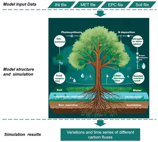
Figure 1.
Ecosystem carbon cycle and Biome-BGCMuSo model structure.

Table 1.
Categories of model input data.
Initialization file: The model needs to run two initialization files in sequence, namely s.ini and n.ini, which contain basic information such as simulation time, geographical location information of the simulation area, information of the model driving file, and output parameter information. The difference between s.ini and n.ini files is that the former is used in the spin-up phase, with a relatively long simulation time (40 years in this study), while the latter is used in the regular simulation phase.
2.1.2. Observations
In this study, the eddy covariance data of the stations were obtained from National Ecosystem Science Data Center, National Science & Technology Infrastructure of China. (http://www.nesdc.org.cn, accessed on 13 August 2023), which usually contains flux data at 30-min, daily, monthly, and annual scales. The eddy covariance technique is a widely recognized method observing fluxes of energy and material exchange between vegetation canopies and atmosphere [23]. Modern eddy correlation techniques could measure NEE directly. Based on the carbon flux data obtained from eddy observations, NEE can be directly obtained. GPP and RE can be calculated separately from NEE in this study, because vegetation does not photosynthesize at night without light, and the NEE at night is regarded as ecosystem respiration.
2.1.3. Spatial Products
Remote sensing spatial products provide long-term, multi-dimensional information for this study. By extracting site information, they can be used as input data to drive the model.
Meteorological data: Climate data were obtained from the National Centers for Environmental Information (NCEI) (https://www.ncei.noaa.gov, accessed on 17 August 2023). The data of national meteorological station were obtained from 1975 to 2020. The datasets include daily total precipitation, daily mean temperature, daily maximum temperature, daily minimum temperature, mean wind speed, and relative air humidity. Meteorological data during 1975–2020 (daily precipitation, Tmax/Tmin) were obtained from NCEI. Linear interpolation was used to address missing records by the values of adjacent days if the temporal gaps were less than 5 consecutive days; for more than 5 consecutive days, gaps were filled with 30-year monthly climatology from the same station. Spatial consistency was conducted by cross-validation against WorldClim v2.1 (1 km resolution) products, which were produced by quantile mapping to correct systematic biases in precipitation extremes [24].
According to the format requirements in the Biome-BGCMuSo model for meteorological data, we selected three meteorological indicators, including maximum temperature, minimum temperature, and precipitation. These indicators were input into the mountain microclimate simulation model (MT-CLIM). Whole meteorological data were then input to MT-CLIM 4.3 to generate daily surface radiation and humidity, with elevation-adjusted lapse rates (−6.5 °C/km for temperature).
Vegetation types data: The driving data of Biome-BGCMuSo model also require ecophysiological parameters of vegetation and soil data. The EPC file is a critical document that describes the physiological and ecological parameters of vegetation and contains default parameters for seven vegetation types: evergreen broadleaf forest, evergreen needleleaf forest, deciduous broadleaf forest, deciduous needleleaf forest, C3 grassland, C4 grassland, and shrubs. These parameters are universal empirical values based on extensive field surveys and synthesizing many previous studies [25].
Soil data: Soil data were from Soil SubCenter, National Earth System Science Data Center, National Science & Technology Infrastructure of China (https://soil.geodata.cn, accessed on 17 August 2023). The soil depth, sand percentage, silt percentage, and soil PH data were extracted based on the latitude and longitude of the site and used to drive the soil module of the model.
2.2. Fluxnet Sites
To correct the Biome-BGCMuSo model and evaluate the efficacy of parameter optimization, observational data from sites were selected from the flux observation network. Eddy covariance has been considered as an effective method for observing time series carbon exchange. A key advantage of this technique exists in directly measuring fluxes across entire ecosystems. Fluxnet is an international network that connects regional networks of Earth system scientists. The third generation of these series, Fluxnet 2015, currently comprises 212 official sites. Each site recorded fluxes of carbon, water, energy, and other ecosystem and biometeorological variables. Combined analysis of flux data from these sites can provide valuable insights into the ecosystem, climate change, and land-use change issues. At present, the Fluxnet network aggregates and disseminates eddy covariance data, encompassing flux networks such as AmeriFlux, AfriFlux, AsiaFlux, and ChinaFlux, among others.
The China Flux Observation and Research Network of Terrestrial Ecosystems (ChinaFLUX), anchored within the Chinese Academy of Sciences, deploys advanced micrometeorological techniques, including eddy covariance and gas chromatography, to monitor the diurnal, seasonal, and inter-annual exchanges of CO2, water vapor, and energy fluxes between China’s quintessential terrestrial ecosystems and the atmosphere [26]. By screening out the outliers and ensuring that these sites are in tropical China, there were 4 sites left with good data quality (Table 2), including two natural and two rubber plantation sites. Forest flux observations were obtained to calibrate and verify the model simulations. The site distribution is shown in Figure 2.
Table 2.
Site descriptions.
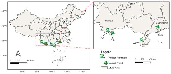
Figure 2.
Site distribution of four tropical forests sites: two natural forest sites (DHS and X_a) and two rubber plantation sites (DZ and X_b).
2.2.1. Natural Forest Sites (DHS Site and X_a Site)
Natural forests are commonly defined as forests that have either not been subjected to human interference, or have been minimally influenced by human activity, where the ecological processes are predominantly driven by natural forces [30]. In this study, there are two natural forest sites, including DHS site (23°10′ N, 112°32′ E) and X_a site (21°36′ N, 101°34′ E).
DHS site is located in Dinghushan Reserve, Zhaoqing City, Guangdong Province, China. The main vegetation type at the site is evergreen broad-leaved forest, belonging to the southern subtropical monsoon humid climate. The site experiences seasonal variations in temperature, with an average annual temperature of 20.9 °C and 1900 mm of rainfall. The soil type is defined as acrisols in World Reference Base for Soil Resources (WRB), with a soil layer depth of 60–90 cm.
The X_a site (Xishuangbanna Tropical Rainforest Flux Site) is in the southern part of Yunnan Province in southwest China, with the soil type defined as ferralsols in WRB. The average annual temperature is 21.8 °C, and the annual precipitation is 1493 mm, mainly concentrating in the rainy season (May to October). The special geomorphology and local climate have led to the development of vegetation types such as tropical rainforests, tropical seasonal wet forests, tropical monsoon rainforests, and tropical montane evergreen broadleaf forests.
2.2.2. Rubber Plantation Sites (DZ Site and X_b Site)
Rubber plantations are typically characterized as cultivated areas of Hevea brasiliensis trees, grown specifically for the production of natural rubber [31]. These plantations have distinct economic significance, primarily harvested for rubber extraction. Two rubber plantation sites are selected for carbon simulation including DZ site and X_b site, located in Hainan Island and Yunnan Province, respectively.
DZ site is located in the northwest of Hainan Island, which experiences two distinct seasons: the wet season from May to October, and the dry season from November to April. The average annual temperature is 21.5~28.5 °C, and the average annual rainfall is 1607 mm, with July, August, and September receiving the majority of this total, accounting for more than 70% of the annual rainfall. Bowfruit millet (Cyrtococcum Patens), airplane grass (Eupatorium odoratum), Xiao Fantian (Urena lobata), and other plants make up most of the understory herbaceous vegetation. The soil type was defined as ferralsols in WRB.
The Xishuangbanna rubber plantation site(X_b) is in the artificial community test area of Xishuangbanna Tropical Forest Ecosystem Research Station of the Chinese Academy of Sciences. It is a single-optimized artificial community dominated by 30-year-old rubber forests, with a planting pattern of wide and narrow rows and dense planting (plant spacing of 3.1 m, narrow rows spacing of 2.5 m, and wide rows spacing of 19.0 m), with a height of 20~30 m, and the planting density of rubber trees being 370 plants hm−2. The soil type was defined as ferralsols in WRB.
2.3. Methods
2.3.1. Sensitivity Analysis
Sensitivity analysis aims to select the most influential ecophysiological parameters of the model [25]. We selected 51 physiological and ecological parameters (Table A1) and chose 20% as the sensitivity interval. We generated multiple sets of inputs and their corresponding output datasets through Monte Carlo simulation [32], and statistically analyzed the sensitivity information about the effect of input parameter variations. Multiple linear regression has been widely used in sensitivity analysis due to its computational simplicity and sensitivity [33]. Standardized regression coefficients are used when the input factors have different units of measure. The linear least squares estimation of the regression coefficients is a measure of sensitivity with the following formula:
where denotes the sensitivity of the ith parameter, denotes the regression coefficient, denotes the standard deviation of the ith parameter sampled multiple times, and denotes the standard deviation of the corresponding result Y.
2.3.2. Calibration of Model Parameters
Among numerous parameterization algorithms, parameter estimation (PEST) and Markov chain Monte Carlo (MCMC) are popular in mode calibration. For example, the scheme of Bayesian optimization and Gaussian Process Regression (BO-GPR) has demonstrated superior performance over other parameter calibration algorithms in terrestrial biosphere model optimization [34], particularly when handling high-dimensional parameter space using process-based model like Biome-BGCMuSo.
UltraOpt framework is selected in this study for parametrization of Biome-BGCMuSo model, which combines Bayesian optimization and evolutionary algorithms. In UltraOpt, GPR is applied to model the objective function, and acquisition functions are used to guide sampling to achieve efficient search for the optimal parameter combination [35]. Suppose we want to fit a function f(x), then the Gaussian process assumes that for any set of input points x1, x2, …, xn, the corresponding function values f(x1), f(x2), …, f(xn) obey a multivariate Gaussian distribution:
where m(x) is the mean function (commonly assumed to be zero), and k(x,x′) is the covariance function (kernel), which describes the relationship between input points. For a given training dataset , the observed values are modeled as the sum of the target function and Gaussian noise:
where is the variance of the observation noise.
2.3.3. Model Validation
The model behavior can be evaluated with a goodness-of-fit of the simulated data to the observed data. We used the correlation coefficient (r), mean absolute error (MAE), and root mean square error (RMSE) as performance indicators:
where n is the number of observations; and are simulated and observed data, respectively, which can be the variables of GPP, RE, and NEE; and and are the means of variables.
3. Results
3.1. Sensitivity Analysis of Ecophysiological Parameters
For natural forest sites, both the DHS and X_a sites showed a sensitivity to SLA and k in carbon fluxes (Figure 3), yet there were still nuances differentiated. RE at the DHS site aligned closely with its GPP parameters, primarily influenced by k and SLA (16.17 and 45.71). SLA denotes the area of a leaf per unit of dry weight and reflects the photosynthetic capacity and resource utilization strategy of the leaf. The k is a coefficient that describes the degree of attenuation of light as it passes through a plant canopy or leaf, and is an important factor affecting the efficiency of photosynthesis and the use of light energy in an ecosystem. Similarly, at X_a site, the principal sensitivity parameters for RE were mainly LFRT and k (38.38 and 19.75). As for NEE, the DHS site is mainly affected by SLA and k (51.29 and 17.03). Conversely, the parameter exerting the most obvious impact on NEE at X_a is the MRpern, with a sensitivity of 61.78. In essence, k and SLA were identified as the key sensitivity parameters for carbon flux variations at DHS, whereas LFRT, k, and MRpern were determinants of carbon flux at the X_a site. The MRpern represents the maintenance respiration coefficient, a linear relationship between tissue N and maintenance respiration, which directly affects GPP and NPP.
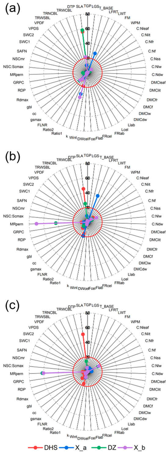
Figure 3.
Sensitivity parameters of Biome-BGCMuSo model for natural and rubber forests. (a), (b), and (c) represent GPP, RE, and NEE, respectively. The length of the line represents the SI. The dotted circles represent the sensitivity, which are 0, 20, 40, 60, and 80 respectively. Red circle represents sensitivity of 20.
Notably, for rubber plantation sites, GPP showed great sensitivity to k, marked at 35.12. The primary sensitivity parameter for RE is the MRpern, with sensitivity values at DZ and X_b sites being 43.4 and 69.83, respectively. Importantly, this parameter also crucially influences NEE variations in these sites, with sensitivities of 61.49 and 60.21. Overall, SLA and k emerged as the chief sensitivity parameters for the rubber plantations’ GPP, while MRpern was pivotal for both RE and NEE.
3.2. Calibration and Validation of Biome-BGCMuSo
A Bayesian optimization approach was used to fine-tune the sensitivity parameters (SI greater than 20%) to localize the Biome-BGCMuSo model. Depending on the a priori model, the Bayesian method estimates afterward parameter values and determines the next samples depending on the available data and the degree of model construction confidence. In this experiment, the Bayesian algorithm will resample 200 times inside a specific parameter space, with 100 iterations at each site.
The simulated daily carbon fluxes for the natural forest from the calibrated Biome-BGCMuSo were validated against observations (Figure 4). The default parameters overestimated GPP and RE for the tropical natural forest. After calibration, the simulations fitted well with the observations. The average value of accuracy (RMSE) for the two natural forest sites basically increased by about 50%. In particular, the DHS site showed the most obvious improvement, probably because of the monoculture of forest types in the area, and the model was able to well simulate the growing progress of natural forests. For the DHS site, the RMSE of GPP and RE decreased significantly, from 6.62 to 1.25 , and 6.79 to 0.72 , respectively. The RMSE of GPP at the DHS site descended by 81.2%, the RMSE of RE descended by 89.4%, and the RMSE of NEE descended by 10.7%, indicating that the localized Biome-BGCMuSo model may greatly enhance the simulation accuracy of tropical natural forests.
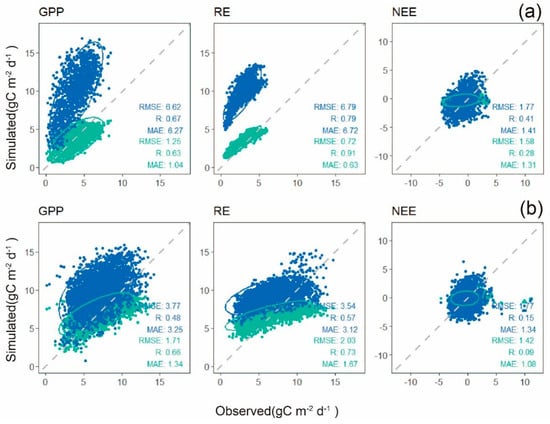
Figure 4.
Scatter plots of simulated daily carbon flux and observed daily carbon flux by the eddy covariance system at DHS site (a) and X_a site (b). The blue points are simulated with original parameters while green points are simulated with calibrated parameters. The number of samples in DHS site is 1460, and 2920 in X_a site. The units of RMSE and MAE are .
The X_a site is a tropical natural rainforest ecosystem with complex forest types, and the calibrated parameters simulated the carbon fluxes well for a complex ecosystem. The RMSE of total GPP decreased from 3.77 to 1.71 , r increased from 0.48 to 0.66, and MAE decreased from 3.25 to 1.34 . The RMSE of total RE decreased from 3.54 to 2.03 , r increased from 0.57 to 0.73, and MAE decreased from 3.12 to 1.67 . The RMSE of total NEE decreased from 1.77 to 1.42 , and MAE decreased from 1.34 to 1.08 . At the X_a site, the RMSE of GPP was decreased by 54.6%, 42.6% for RE and 19.8% for NEE.
Compared to the tropical natural forests, the localized Biome-BGCMuSo model for the two rubber forest sites did not perform as well in the simulation.
As seen from Figure 5a, the localized model performed better with more closely to the observed values as compared with the default parameters of rubber plantations at the DZ site, with the RMSE decreased by about 62.8% for GPP, 68.1% for RE, and 13.8% for NEE. The RMSE of the total GPP decreased from 5.95 to 2.21 , r increased from 0.3 to 0.52, and the MAE decreased from 5.45 to 1.74 . The RMSE of the RE decreased from 4.04 to 1.29 , r increased from 0.46 to 0.66, and the MAE decreased from 3.75 to 1.02 . The RMSE of NEE decreased from 2.39 to 2.06 , r increased from 0.05 to 0.25, and MAE decreased from 1.99 to 1.67 .
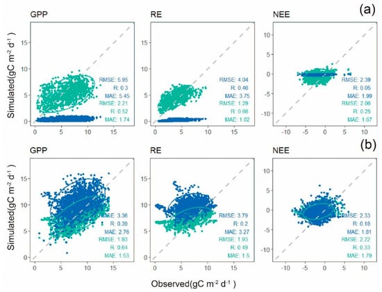
Figure 5.
Scatter plots of simulated daily carbon flux and observed daily carbon flux by the eddy covariance system at DZ site (a) and X_b site (b). The blue points are simulated with original parameters while green points are simulated with calibrated parameters. The number of samples in DZ site is 1073, and1460 in X_b site. The units of RMSE and MAE are .
At the X_b site, the RMSE of GPP decreased by 42.5%, while it decreased by 49.1% for RE and 0.05% for NEE with the localized Biome-BGCMuSo model. The RMSE of the GPP in the X_b site dropped from 3.36 to 1.93 , r increased from 0.39 to 0.64, and the MAE dropped from 2.76 to 1.53 . The RMSE and MAE of the RE dropped from 3.79 to 1.93 and 3.27 to 1.5 , respectively. And the value of r increased from 0.2 to 0.49. For NEE, the RMSE and MAE dropped from 2.33 to 2.22 and 1.81 to 1.79 , respectively, and the value of r increased from 0.18 to 0.33.
To further explore the accuracy of the localized model, we compared the annual values of measured and simulated carbon fluxes (Figure 6). The results show that the standard deviation of GPP for site DHS was 83.44 , the standard deviation of RE was 104.44 , and the standard deviation of NEE was 95.39 . The standard deviation of GPP for site X_a was 202.33 , the standard deviation of RE was 188.91 , and the standard deviation of NEE was 56.61 . For the plantation forest, the standard deviation of GPP for site DZ was 181.99 , the standard deviation of RE was 182.78 and NEE was 264.11 . For site X_b, the standard deviation of GPP was 266.38 , RE was 382.66 and NEE was 255.02 . In comparison, the values simulated for the natural forests (DHS and X_a) were closer to the original flux data with a lower standard deviation.
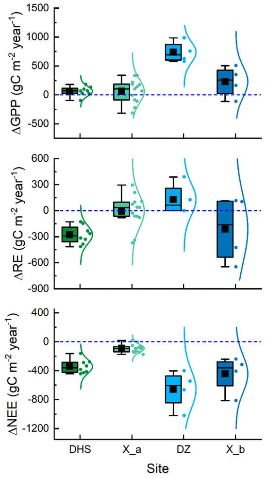
Figure 6.
Standard deviation of annual values for observed and simulated carbon fluxes during 2000 to 2018.
3.3. Inter-Annual and Intra-Annual Carbon Flux Variation of Natural and Planted Rubber Forests
Annual carbon fluxes for the four sites were calculated and performed in Figure 7. With the localized model, we simulated the carbon flux data of each site over the years and made inter-annual comparisons with the observed data. Figure 7 shows the inter-annual variation in GPP at tropical sites from 2000 to 2018 (the DZ site starts from 2001 because rubber forest planting started in 2001 in the region). From the simulation results, the GPP values of both natural and plantation forest sites (X_a and X_b) in the Xishuangbanna region are relatively high, and the values of DHS and DZ are relatively low. The GPP of the three sites showed an increasing trend during 2000 and 2016, except for DHS. The inter-annual trend of RE was similar to that of GPP. For natural forests, the inter-annual changes in simulated NEE at DHS showed that its carbon sink capacity was gradually weakening, and the carbon sink capacity of natural forests in Xishuangbanna was also gradually weakening. The carbon sink capacity of the planted forest (DZ and X_b) sites was both stronger than that of the natural forest, with NEE changes fluctuating within a range of fluctuate.
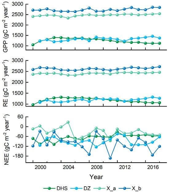
Figure 7.
Simulated annual carbon flux of four sites by localized Biome-BGCMuSo model from 2000 to 2018.
The carbon fluxes of tropical natural forests and rubber plantations, as simulated by Biome-BGCMuSo, are displayed in Figure 8. Simulations and observations of GPP revealed seasonal consistency at the four sites. In the summer, daily photosynthesis peaks and GPP rises to a maximum under favorable environmental conditions; in the winter, GPP is smaller or even negligible because photosynthesis in ecosystems is limited by low temperatures and weak solar radiation during this season. Photosynthesis in biomes is essentially not exactly zero because mixed and evergreen forests dominate vegetative ecosystems in the tropics. RE, which includes heterotrophic, growth, and maintenance respiration, is closely related with photosynthesis in ecosystems. These are the two opposing directions of carbon fluxes in ecosystems during carbon uptake and release. RE usually follows the same pattern as GPP.
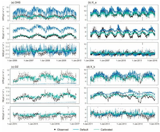
Figure 8.
Temporal variation in daily GPP, RE, and NEE of observed and simulated carbon flues at four sites. Black points represent observed data, values in blue line represent simulated values with default parameters, and values in green line represent simulated values with calibrated parameters.
As the difference between GPP and RE, the NEE is used to represent the net carbon exchange between ecosystems and the atmosphere. However, because the model-simulated NEE values were more continuous and could not more accurately reflect the net carbon exchange between ecosystems, as well as having bigger MAE and RMSE, the error of the simulated NEE was greater than that of the simulated GPP. The tropical forest ecosystems in China were shown by both simulated and observed NEE to be carbon sinks in the summer and carbon sources in the winter. The variation characteristics of carbon exchange at the seasonal scale are more obvious in NEE simulated by Biome-BGCMuSo than those observed.
4. Discussion
Modeling carbon fluxes in tropical forests via process-based models is beset with significant challenges, owing to the intricate nature of these ecosystems, the imperative for precise model parameterization, and the necessity to incorporate the impacts of disturbances. To improve the accuracy of carbon flux simulations and simplify the complexity of ecosystem process-based model parameters, the novelty of our study lies in the sensitivity analyses of physiological and ecological parameters of vegetation in both rubber plantations and natural tropical forests, and the correction of sensitivity parameters to improve the accuracy of model simulations.
Overall, the common sensitivity parameters for both natural and plantation forests include SLA, k, and MRpern. According to linear least squares estimation, the key sensitivity parameters for GPP between natural and plantation forests in Biome-BGCMuSo are SLA and k. Previous studies have also demonstrated this result [25,36]. A machine learning study has further confirmed that C:Nleaf, SLA, FLNR, and k are both direct and indirect parameters affecting photosynthetic capacity [37]. C:Nleaf and SLA determine the rate of carbon assimilation by Rubisco enzyme quantity, which, along with FLNR, controls the maximum carboxylation rate (Vcmax), fundamental for microbial metabolic decomposition and plant nutrient cycling [38]. The k is defined in the Beer–Lambert law as the nonlinear relationship between the absorbed fraction of photosynthetically active radiation (fPAR) and the leaf area index (LAI); a higher k indicates reduced variability and average of projected radiation. For RE, the main sensitivity parameters are MRpern and SLA, with SLA representing the ratio of single-sided leaf area to dry weight. The relative growth rate and net photosynthetic rate of leaves are proportional to SLA, with high SLA plants typically found in resource-rich environments. MRpern represents the maintenance respiration coefficient, a linear relationship between tissue N and maintenance respiration, which directly affects GPP and NPP [39]. Vegetation respiration, a key component of ecosystem carbon balance, is susceptible to environmental factors [40].
Ecosystem process-based models generally provide a better simulation of key processes such as vegetation growth, carbon uptake and release, and contribute to our understanding of ecosystem dynamics in tropical forests [41,42]. Figure 7 and Figure 8 demonstrated the strong carbon sequestration capacity of plantations. The strong carbon sink in rubber plantations may arise from forest age and carbon allocation trade-offs. Rubber plantations’ even-aged structure (30-year rotation) maximizes mid-rotation carbon uptake, contrasting with natural forests’ mixed-age mortality patterns [43]. And as for carbon allocation, about 23% of plantation NPP is allocated to latex production (non-structural carbon), transiently inflating NEE compared to natural forests’ woody biomass sequestration [44]. In Figure 4 and Figure 5, the calibrated simulations show that the default parameters exhibit a more pronounced overestimation when assessing GPP and RE in both natural and planted forests. The localized model performs better in assessing GPP and RE, but the simulated NEE will be lower than the measured value, resulting in an underestimation of ecosystem carbon sink capacity. The first phase in running a Biome-BGC model is rotation, which requires stable beginning conditions to ensure that input and output fluxes are in equilibrium [45]. Taken together, among these sites, the carbon flux simulation results of natural forests in Xishuangbanna are relatively the best. The superior performance of Biome-BGCMuSo in natural forests can be attributed to these key ecological factors. Natural forests’ multi-layered canopy buffers microclimate variability, aligning better with the model’s light attenuation assumptions [46]. And century-old organic horizons stabilize microbial respiration rates, reducing parameterization uncertainty [47].
Although the Biome-BGCMuSo model performs better in the tropics after local validation compared to non-localization, there are still some uncertainties, including inaccuracies in meteorological data, uncertainties in the model structure, and the diversity of vegetation types [48,49,50]. The accuracy of meteorological data is critical to the quality of model simulations because models rely on these data to simulate climate impacts on ecosystems, and errors or incompleteness in meteorological data can lead to biases in the model’s simulation of ecological processes. The meteorological data are obtained by using the collected daily maximum and minimum temperatures, precipitation, and other data of the station, and processed by MT-CLIM 4.3, so there is a certain degree of uncertainty in the meteorological data. The model itself is also an aspect to be considered. The Biome-BGCMuSo model is a structurally complex ecosystem model that simulates multiple processes in a coupled fashion, and a single computational equation may involve multiple parameters, resulting in a high sensitivity to parameters [46]. In addition, the applicability of the model in tropical forests may be affected by vegetation types and geographic differences [51]. As for the tropics, the types of vegetation are complex and the ecosystems have a mixture of tree species, so the diversity of vegetation types is one of the sources of uncertainty that leads to the bias of the model simulation results [5]. For plantation forests, studies have also been conducted to adjust the physiological and ecological parameters of vegetation based on genetic algorithms, and high simulation accuracies have been obtained [52]. Therefore, tuning of ecosystem process-based models using machine learning algorithms to adjust simulated values can contribute to higher accuracy model simulations.
Natural tropical forests, distinguished by their rich biodiversity and intricate ecosystem structures, demonstrate robust resistance to disturbances and exhibit minimal perturbations in their role as carbon sinks [53]. Contrastingly, rubber plantations are frequently characterized by their enhanced carbon sequestration capacity and economic value, yet this is accompanied by a diminished level of biodiversity [54]. Goal 15 of the United Nations Sustainable Development Goals underscores the imperative to protect, restore, and promote the sustainable usage of terrestrial ecosystems, judiciously manage forests, combat desertification, halt and reverse land degradation, and cease the loss of biodiversity. Consequently, identifying a strategy to equilibrate the rapid expansion of economic forestry with the services provided by ecosystems is an exigent challenge that necessitates immediate attention. In future studies, we hope to validate the parameters and structure of the model with more field observation data to verify the localization effect of the model. For plantation forests, it is important to obtain as much information on anthropogenic management as possible, and use the unique anthropogenic management module of Biome-BGCMuSo to study the carbon cycle process of plantation forest ecosystems, and quantify the contribution of anthropogenic management to carbon sequestration.
5. Conclusions
The forest carbon cycle has strong regional heterogeneity, and the sensitivity parameters of different forest types are inconsistent. Therefore, the use of EC data can better calibrate the ecological process model. To evaluate and improve the performances of the Biome-BGCMuSo model in natural and planted forests for tropical regions, we used a machine learning method to calibrate the parameters of the Biome-BGCMuSo model. The sensitivity parameters were first tested, and the model calibration using a Bayesian machine learning algorithm was conducted in this study. We concluded that the sensitivity of vegetation physiological and ecological parameters varied among natural and planted forests. The common sensitivity parameters for both natural and plantation forests include specific leaf area (SLA), extinction coefficient (k), and maintenance respiration per nitrogen (MRpern). The calibrated model significantly improved the performances of carbon fluxes at both natural and planted forest sites with the average accuracy increased by 60.23%. Anthropogenic management led to large differences in carbon flux simulation of natural and planted forests, and the localized Biome-BGCMuSo model performed better in natural forest sites than in planted sites.
Tropical natural forests, with their rich biodiversity and intricate ecosystems, are indispensable in the global carbon cycle. These forests excel in sequestering carbon, thereby playing a crucial role in mitigating climate change and enhancing resilience against environmental fluctuations. The value of carbon stored in these forests extends beyond ecological benefits, as it also holds significant economic potential through carbon credits and sustainable forest management practices. On the other hand, rubber plantations, while exhibiting high carbon storage capacity, tend to support lower biodiversity. Despite this limitation, their contribution to carbon sequestration remains noteworthy, particularly in regions where natural forests have been depleted. The economic value of carbon in rubber plantations can also be harnessed through well-regulated carbon markets and sustainable land-use policies.
Author Contributions
Conceptualization: L.Z.; formal analysis: F.Y.; writing—original draft: F.Y.; supervision: L.Z. and M.Y.; writing—review and editing: L.Z. and B.C.; funding acquisition: L.Z.; methodology: M.Y.; validation: M.Y. and B.C.; data curation: L.R. All authors have read and agreed to the published version of the manuscript.
Funding
This work was financially supported by the Provincial Natural Science Foundation of Hainan (724CXTD434).
Data Availability Statement
The data presented in this study are available on request from the corresponding author (M.Y.).
Acknowledgments
The authors also thank ChinaFLUX for providing the eddy covariance dataset product.
Conflicts of Interest
The authors declare no conflicts of interest.
Appendix A
Table A1.
Candidate parameters of Biome-BGCMuSo model for sensitivity analysis.
Table A1.
Candidate parameters of Biome-BGCMuSo model for sensitivity analysis.
| Number | Parameters | Abbreviation | Default Value | Units |
|---|---|---|---|---|
| 1. | transfer growth period as fraction of growing season (when transferGDD_flag = 0) | TGP | 0.2 | prop. |
| 2. | litterfall as fraction of growing season (when transferGDD_flag = 0) | LGS | 0.2 | prop |
| 3. | base temperature | T_BASE | 0 | Celsius |
| 4. | annual leaf and fine root turnover fraction | LFRT | 0.2 | 1/year |
| 5. | annual live wood turnover fraction | LWT | 0.70 | 1/year |
| 6. | annual fire mortality fraction | FM | 0.00 | 1/year |
| 7. | whole-plant mortality fraction in vegetation period | WPM | 0.001 | 1/vegper |
| 8. | C:N of leaves | C:Nleaf | 42.0 | kgC/kgN |
| 9. | C:N of leaf litter, after retranslocation | C:Nlit | 49.0 | kgC/kgN |
| 10. | C:N of fine roots | C:Nfr | 42.0 | kgC/kgN |
| 11. | C:N of fruit | C:Nf | 46.6 | kgC/kgN |
| 12. | C:N of soft stem | C:Nss | 46.6 | kgC/kgN |
| 13. | C:N of live wood | C:Nlw | 50.0 | kgC/kgN |
| 14. | C:N of dead wood | C:Ndw | 300.0 | kgC/kgN |
| 15. | dry matter carbon content of leaves | DMCleaf | 0.4 | kgC/kgDM |
| 16. | dry matter carbon content of leaf litter | DMClit | 0.4 | kgC/kgDM |
| 17. | dry matter carbon content of fine roots | DMCfr | 0.4 | kgC/kgDM |
| 18. | dry matter carbon content of fruit | DMCf | 0.4 | kgC/kgDM |
| 19. | dry matter carbon content of live wood | DMClw | 0.4 | kgC/kgDM |
| 20. | dry matter carbon content of dead wood | DMCdw | 0.4 | kgC/kgDM |
| 21. | leaf litter labile proportion | Llab | 0.32 | DIM |
| 22. | leaf litter cellulose proportion | Lcel | 0.44 | DIM |
| 23. | fine root labile proportion | FRlab | 0.30 | DIM |
| 24. | fine root cellulose proportion | FRcel | 0.45 | DIM |
| 25. | fruit litter labile proportion | Flab | 0.68 | DIM |
| 26. | fruit litter cellulose proportion | Fcel | 0.23 | DIM |
| 27. | dead wood cellulose proportion | DWcel | 0.76 | DIM |
| 28. | canopy water interception coefficient | Wint | 0.041 | 1/LAI/d |
| 29. | canopy light extinction coefficient | k | 0.7 | DIM |
| 30. | all-sided to projected leaf area ratio | Ratio1 | 2.0 | DIM |
| 31. | ratio of shaded SLA/sunlit SLA | Ratio2 | 2.0 | DIM |
| 32. | fraction of leaf N in Rubisco | FLNR | 0.06 | DIM |
| 33. | maximum stomatal conductance (projected area basis) | gsmax | 0.005 | m/s |
| 34. | cuticular conductance (projected area basis) | cc | 0.00001 | m/s |
| 35. | boundary layer conductance (projected area basis) | gbl | 0.01 | m/s |
| 36. | maximum depth of rooting zone | Rdmax | 2.0 | m |
| 37. | root distribution parameter | RDP | 2.0 | DIM |
| 38. | growth resp per unit of C grown | GRPC | 0.3 | prop |
| 39. | maintenance respiration in kgC/day per kg of tissue N | MRpern | 0.218 | kgC/kgN/d |
| 40. | theoretical maximum prop. of non-structural and structural carbohydrates | NSC:Scmax | 0.1 | DIM |
| 41. | prop. of non-structural carbohydrates available for maintanance respiration | NSCmr | 0.1 | DIM |
| 42. | symbiotic + asymbiotic fixation of N | SAFN | 0.0015 | kgN/m2/year |
| 43. | VWC ratio to calc. soil moisture limit 1 (prop. to FC-WP) | SWC1 | 0.3 | prop |
| 44. | VWC ratio to calc. soil moisture limit 2 (prop. to SAT-FC) | SWC2 | 0.99 | prop |
| 45. | vapor pressure deficit: start of conductance reduction | VPDS | 1800 | Pa |
| 46. | vapor pressure deficit: complete conductance reduction | VPDF | 4800 | Pa |
| 47. | turnover rate of wilted standing biomass to litter | TRWSBL | 0.01 | prop |
| 48. | turnover rate of non-woody cut-down biomass to litter | TRNCBL | 0.01 | prop |
| 49. | turnover rate of woody cut-down biomass to litter | TRWCBL | 0.0009 | prop |
| 50. | drought tolerance parameter (critical value of DSWS) | DTP | 30 | nday |
| 51. | canopy average specific leaf area (projected area basis) | SLA | 8 | m2/kgC |
References
- Pan, Y.; Birdsey, R.A.; Phillips, O.L.; Jackson, R.B. The Structure, Distribution, and Biomass of the World’s Forests. Annu. Rev. Ecol. Evol. Syst. 2013, 44, 593–622. [Google Scholar] [CrossRef]
- Mo, L.; Zohner, C.M.; Reich, P.B.; Liang, J.; De Miguel, S.; Nabuurs, G.-J.; Renner, S.S.; Van Den Hoogen, J.; Araza, A.; Herold, M.; et al. Integrated Global Assessment of the Natural Forest Carbon Potential. Nature 2023, 624, 92–101. [Google Scholar] [CrossRef] [PubMed]
- Yu, K.; Ciais, P.; Seneviratne, S.I.; Liu, Z.; Chen, H.Y.H.; Barichivich, J.; Allen, C.D.; Yang, H.; Huang, Y.; Ballantyne, A.P. Field-Based Tree Mortality Constraint Reduces Estimates of Model-Projected Forest Carbon Sinks. Nat. Commun. 2022, 13, 2094. [Google Scholar] [CrossRef] [PubMed]
- Pan, Y.; Birdsey, R.A.; Fang, J.; Houghton, R.; Kauppi, P.E.; Kurz, W.A.; Phillips, O.L.; Shvidenko, A.; Lewis, S.L.; Canadell, J.G.; et al. A Large and Persistent Carbon Sink in the World’s Forests. Science 2011, 333, 988–993. [Google Scholar] [CrossRef]
- Powers, J.S.; Marín-Spiotta, E. Ecosystem Processes and Biogeochemical Cycles in Secondary Tropical Forest Succession. Annu. Rev. Ecol. Evol. Syst. 2017, 48, 497–519. [Google Scholar] [CrossRef]
- Mitchard, E.T.A. The Tropical Forest Carbon Cycle and Climate Change. Nature 2018, 559, 527–534. [Google Scholar] [CrossRef]
- Grainger, A.; Malayang, B.S. A Model of Policy Changes to Secure Sustainable Forest Management and Control of Deforestation in the Philippines. For. Policy Econ. 2006, 8, 67–80. [Google Scholar] [CrossRef]
- Liu, J.; Bowman, K.W.; Schimel, D.S.; Parazoo, N.C.; Jiang, Z.; Lee, M.; Bloom, A.A.; Wunch, D.; Frankenberg, C.; Sun, Y.; et al. Contrasting Carbon Cycle Responses of the Tropical Continents to the 2015–2016 El Niño. Science 2017, 358, eaam5690. [Google Scholar] [CrossRef]
- Feng, Y.; Zeng, Z.; Searchinger, T.D.; Ziegler, A.D.; Wu, J.; Wang, D.; He, X.; Elsen, P.R.; Ciais, P.; Xu, R.; et al. Doubling of Annual Forest Carbon Loss over the Tropics during the Early Twenty-First Century. Nat. Sustain. 2022, 5, 444–451. [Google Scholar] [CrossRef]
- Hofhansl, F.; Chacón-Madrigal, E.; Fuchslueger, L.; Jenking, D.; Morera-Beita, A.; Plutzar, C.; Silla, F.; Andersen, K.M.; Buchs, D.M.; Dullinger, S.; et al. Climatic and Edaphic Controls over Tropical Forest Diversity and Vegetation Carbon Storage. Sci. Rep. 2020, 10, 5066. [Google Scholar] [CrossRef]
- Li, Z.; Ahlström, A.; Tian, F.; Gärtner, A.; Jiang, M.; Xia, J. Minimum Carbon Uptake Controls the Interannual Variability of Ecosystem Productivity in Tropical Evergreen Forests. Glob. Planet. Change 2020, 195, 103343. [Google Scholar] [CrossRef]
- Lawrence, D.M.; Fisher, R.A.; Koven, C.D.; Oleson, K.W.; Swenson, S.C.; Bonan, G.; Collier, N.; Ghimire, B.; van Kampenhout, L.; Kennedy, D.; et al. The Community Land Model Version 5: Description of New Features, Benchmarking, and Impact of Forcing Uncertainty. J. Adv. Model. Earth Syst. 2019, 11, 4245–4287. [Google Scholar] [CrossRef]
- Guimberteau, M.; Zhu, D.; Maignan, F.; Huang, Y.; Yue, C.; Dantec-Nédélec, S.; Ottlé, C.; Jornet-Puig, A.; Bastos, A.; Laurent, P.; et al. ORCHIDEE-MICT (v8.4.1), a Land Surface Model for the High Latitudes: Model Description and Validation. Geosci. Model. Dev. 2018, 11, 121–163. [Google Scholar] [CrossRef]
- Ahlström, A.; Raupach, M.R.; Schurgers, G.; Smith, B.; Arneth, A.; Jung, M.; Reichstein, M.; Canadell, J.G.; Friedlingstein, P.; Jain, A.K.; et al. The Dominant Role of Semi-Arid Ecosystems in the Trend and Variability of the Land CO2 Sink. Science 2015, 348, 895–899. [Google Scholar] [CrossRef]
- Hidy, D.; Barcza, Z.; Hollós, R.; Dobor, L.; Ács, T.; Zacháry, D.; Filep, T.; Pásztor, L.; Incze, D.; Dencső, M.; et al. Soil-Related Developments of the Biome-BGCMuSo v6.2 Terrestrial Ecosystem Model. Geosci. Model. Dev. 2022, 15, 2157–2181. [Google Scholar] [CrossRef]
- Erb, K.-H.; Fetzel, T.; Plutzar, C.; Kastner, T.; Lauk, C.; Mayer, A.; Niedertscheider, M.; Körner, C.; Haberl, H. Biomass Turnover Time in Terrestrial Ecosystems Halved by Land Use. Nat. Geosci. 2016, 9, 674–678. [Google Scholar] [CrossRef]
- Mao, F.; Zhou, G.; Li, P.; Du, H.; Xu, X.; Shi, Y.; Mo, L.; Zhou, Y.; Tu, G. Optimizing Selective Cutting Strategies for Maximum Carbon Stocks and Yield of Moso Bamboo Forest Using BIOME-BGC Model. J. Environ. Manag. 2017, 191, 126–135. [Google Scholar] [CrossRef]
- Brinck, K.; Fischer, R.; Groeneveld, J.; Lehmann, S.; Dantas De Paula, M.; Pütz, S.; Sexton, J.O.; Song, D.; Huth, A. High Resolution Analysis of Tropical Forest Fragmentation and Its Impact on the Global Carbon Cycle. Nat. Commun. 2017, 8, 14855. [Google Scholar] [CrossRef]
- Liu, S.; Bond-Lamberty, B.; Hicke, J.A.; Vargas, R.; Zhao, S.; Chen, J.; Edburg, S.L.; Hu, Y.; Liu, J.; McGuire, A.D.; et al. Simulating the Impacts of Disturbances on Forest Carbon Cycling in North America: Processes, Data, Models, and Challenges. J. Geophys. Res. 2011, 116, G00K08. [Google Scholar] [CrossRef]
- Fischer, R.; Bohn, F.; Dantas de Paula, M.; Dislich, C.; Groeneveld, J.; Gutiérrez, A.G.; Kazmierczak, M.; Knapp, N.; Lehmann, S.; Paulick, S.; et al. Lessons Learned from Applying a Forest Gap Model to Understand Ecosystem and Carbon Dynamics of Complex Tropical Forests. Ecol. Model. 2016, 326, 124–133. [Google Scholar] [CrossRef]
- Ueyama, M.; Ichii, K.; Hirata, R.; Takagi, K.; Asanuma, J.; Machimura, T.; Nakai, Y.; Ohta, T.; Saigusa, N.; Takahashi, Y.; et al. Simulating Carbon and Water Cycles of Larch Forests in East Asia by the BIOME-BGC Model with AsiaFlux Data. Biogeosciences 2010, 7, 959–977. [Google Scholar] [CrossRef]
- Hidy, D.; Barcza, Z.; Haszpra, L.; Churkina, G.; Pintér, K.; Nagy, Z. Development of the Biome-BGC Model for Simulation of Managed Herbaceous Ecosystems. Ecol. Model. 2012, 226, 99–119. [Google Scholar] [CrossRef]
- Velasco, E.; Roth, M. Cities as Net Sources of CO2: Review of Atmospheric CO2 Exchange in Urban Environments Measured by Eddy Covariance Technique: Urban CO2 Flux Measurements by Eddy Covariance. Geogr. Compass 2010, 4, 1238–1259. [Google Scholar] [CrossRef]
- Fick, S.E.; Hijmans, R.J. WorldClim 2: New 1-Km Spatial Resolution Climate Surfaces for Global Land Areas. Int. J. Climatol. 2017, 37, 4302–4315. [Google Scholar] [CrossRef]
- White, M.A.; Thornton, P.E.; Running, S.W.; Nemani, R.R. Parameterization and Sensitivity Analysis of the BIOME–BGC Terrestrial Ecosystem Model: Net Primary Production Controls. Earth Interact. 2000, 4, 1–85. [Google Scholar] [CrossRef]
- Li, S.; Wang, G.; Sun, S.; Chen, H.; Bai, P.; Zhou, S.; Huang, Y.; Wang, J.; Deng, P. Assessment of Multi-Source Evapotranspiration Products over China Using Eddy Covariance Observations. Remote Sens. 2018, 10, 1692. [Google Scholar] [CrossRef]
- Zhou, G.; Houlton, B.Z.; Wang, W.; Huang, W.; Xiao, Y.; Zhang, Q.; Liu, S.; Cao, M.; Wang, X.; Wang, S.; et al. Substantial Reorganization of China’s Tropical and Subtropical Forests: Based on the Permanent Plots. Glob. Change Biol. 2014, 20, 240–250. [Google Scholar] [CrossRef]
- Li, Z.; Zhang, Y.; Wang, S.; Yuan, G.; Yang, Y.; Cao, M. Evapotranspiration of a Tropical Rain Forest in Xishuangbanna, Southwest China. Hydrol. Process. 2010, 24, 2405–2416. [Google Scholar] [CrossRef]
- Sun, R.; Wu, Z.; Lan, G.; Yang, C.; Fraedrich, K. Effects of Rubber Plantations on Soil Physicochemical Properties on Hainan Island, China. J. Environ. Qual. 2021, 50, 1351–1363. [Google Scholar] [CrossRef]
- Chazdon, R.L.; Brancalion, P.H.S.; Laestadius, L.; Bennett-Curry, A.; Buckingham, K.; Kumar, C.; Moll-Rocek, J.; Vieira, I.C.G.; Wilson, S.J. When Is a Forest a Forest? Forest Concepts and Definitions in the Era of Forest and Landscape Restoration. Ambio 2016, 45, 538–550. [Google Scholar] [CrossRef]
- Azizan, F.A.; Kiloes, A.M.; Astuti, I.S.; Abdul Aziz, A. Application of Optical Remote Sensing in Rubber Plantations: A Systematic Review. Remote Sens. 2021, 13, 429. [Google Scholar] [CrossRef]
- Zagayevskiy, Y.; Deutsch, C.V. A Methodology for Sensitivity Analysis Based on Regression: Applications to Handle Uncertainty in Natural Resources Characterization. Nat. Resour. Res. 2015, 24, 239–274. [Google Scholar] [CrossRef]
- Ashley, R.A.; Parmeter, C.F. Sensitivity Analysis of an OLS Multiple Regression Inference with Respect to Possible Linear Endogeneity in the Explanatory Variables, for Both Modest and for Extremely Large Samples. Econometrics 2020, 8, 11. [Google Scholar] [CrossRef]
- Shahriari, B.; Swersky, K.; Wang, Z.; Adams, R.P.; de Freitas, N. Taking the Human Out of the Loop: A Review of Bayesian Optimization. Proc. IEEE 2016, 104, 148–175. [Google Scholar] [CrossRef]
- Falkner, S.; Klein, A.; Hutter, F. BOHB: Robust and Efficient Hyperparameter Optimization at Scale. In Proceedings of the 35th International Conference on Machine Learning, Stockholm, Sweden, 10–15 July 2018. [Google Scholar]
- Raj, R.; Hamm, N.A.S.; van der Tol, C.; Stein, A. Variance-Based Sensitivity Analysis of BIOME-BGC for Gross and Net Primary Production. Ecol. Model. 2014, 292, 26–36. [Google Scholar] [CrossRef]
- Dagon, K.; Sanderson, B.M.; Fisher, R.A.; Lawrence, D.M. A Machine Learning Approach to Emulation and Biophysical Parameter Estimation with the Community Land Model, Version 5. Adv. Stat. Climatol. Meteorol. Oceanogr. 2020, 6, 223–244. [Google Scholar] [CrossRef]
- Ferlian, O.; Wirth, C.; Eisenhauer, N. Leaf and Root C-to-N Ratios Are Poor Predictors of Soil Microbial Biomass C and Respiration across 32 Tree Species. Pedobiologia 2017, 65, 16–23. [Google Scholar] [CrossRef]
- Ryan, M.G. Effects of Climate Change on Plant Respiration. Ecol. Appl. 1991, 1, 157–167. [Google Scholar] [CrossRef]
- O’Leary, B.M.; Asao, S.; Millar, A.H.; Atkin, O.K. Core Principles Which Explain Variation in Respiration across Biological Scales. New Phytol. 2019, 222, 670–686. [Google Scholar] [CrossRef]
- Pan, S.; Tian, H.; Dangal, S.R.S.; Ouyang, Z.; Tao, B.; Ren, W.; Lu, C.; Running, S. Modeling and Monitoring Terrestrial Primary Production in a Changing Global Environment: Toward a Multiscale Synthesis of Observation and Simulation. Adv. Meteorol. 2014, 2014, 965936. [Google Scholar] [CrossRef]
- Bonan, G.B.; Doney, S.C. Climate, Ecosystems, and Planetary Futures: The Challenge to Predict Life in Earth System Models. Science 2018, 359, eaam8328. [Google Scholar] [CrossRef] [PubMed]
- Brienen, R.J.W.; Caldwell, L.; Duchesne, L.; Voelker, S.; Barichivich, J.; Baliva, M.; Ceccantini, G.; Di Filippo, A.; Helama, S.; Locosselli, G.M.; et al. Forest Carbon Sink Neutralized by Pervasive Growth-Lifespan Trade-Offs. Nat. Commun. 2020, 11, 4241. [Google Scholar] [CrossRef] [PubMed]
- Hertel, D.; Moser, G.; Culmsee, H.; Erasmi, S.; Horna, V.; Schuldt, B.; Leuschner, C. Below- and above-Ground Biomass and Net Primary Production in a Paleotropical Natural Forest (Sulawesi, Indonesia) as Compared to Neotropical Forests. For. Ecol. Manag. 2009, 258, 1904. [Google Scholar] [CrossRef]
- Du, L.; Zeng, Y.; Ma, L.; Qiao, C.; Wu, H.; Su, Z.; Bao, G. Effects of Anthropogenic Revegetation on the Water and Carbon Cycles of a Desert Steppe Ecosystem. Agric. For. Meteorol. 2021, 300, 108339. [Google Scholar] [CrossRef]
- Fisher, R.A.; Koven, C.D.; Anderegg, W.R.L.; Christoffersen, B.O.; Dietze, M.C.; Farrior, C.E.; Holm, J.A.; Hurtt, G.C.; Knox, R.G.; Lawrence, P.J.; et al. Vegetation Demographics in Earth System Models: A Review of Progress and Priorities. Glob. Change Biol. 2018, 24, 35–54. [Google Scholar] [CrossRef]
- Powers, J.S.; Corre, M.D.; Twine, T.E.; Veldkamp, E. Geographic Bias of Field Observations of Soil Carbon Stocks with Tropical Land-Use Changes Precludes Spatial Extrapolation. Proc. Natl. Acad. Sci. USA 2011, 108, 6318–6322. [Google Scholar] [CrossRef]
- Melbourne-Thomas, J.; Johnson, C.R.; Fulton, E.A. Characterizing Sensitivity and Uncertainty in a Multiscale Model of a Complex Coral Reef System. Ecol. Model. 2011, 222, 3320–3334. [Google Scholar] [CrossRef]
- Ma, H.; Ma, C.; Li, X.; Yuan, W.; Liu, Z.; Zhu, G. Sensitivity and Uncertainty Analyses of Flux-Based Ecosystem Model towards Improvement of Forest GPP Simulation. Sustainability 2020, 12, 2584. [Google Scholar] [CrossRef]
- Fodor, N.; Pásztor, L.; Szabó, B.; Laborczi, A.; Pokovai, K.; Hidy, D.; Hollós, R.; Kristóf, E.; Kis, A.; Dobor, L.; et al. Input Database Related Uncertainty of Biome-BGCMuSo Agro-Environmental Model Outputs. Int. J. Digit. Earth 2021, 14, 1582–1601. [Google Scholar] [CrossRef]
- Zhang, L.; Xiao, J.; Zhou, Y.; Zheng, Y.; Li, J.; Xiao, H. Drought Events and Their Effects on Vegetation Productivity in China. Ecosphere 2016, 7, e01591. [Google Scholar] [CrossRef]
- Imvitthaya, C. Calibration of a Biome-Biogeochemical Cycles Model for Modeling the Net Primary Production of Teak Forests through Inverse Modeling of Remotely Sensed Data. J. Appl. Remote Sens. 2011, 5, 053516. [Google Scholar] [CrossRef]
- Gough, C.M.; Atkins, J.W.; Bond-Lamberty, B.; Agee, E.A.; Dorheim, K.R.; Fahey, R.T.; Grigri, M.S.; Haber, L.T.; Mathes, K.C.; Pennington, S.C.; et al. Forest Structural Complexity and Biomass Predict First-Year Carbon Cycling Responses to Disturbance. Ecosystems 2021, 24, 699–712. [Google Scholar] [CrossRef]
- Singh, A.K.; Liu, W.; Zakari, S.; Wu, J.; Yang, B.; Jiang, X.J.; Zhu, X.; Zou, X.; Zhang, W.; Chen, C.; et al. A Global Review of Rubber Plantations: Impacts on Ecosystem Functions, Mitigations, Future Directions, and Policies for Sustainable Cultivation. Sci. Total Environ. 2021, 796, 148948. [Google Scholar] [CrossRef] [PubMed]
Disclaimer/Publisher’s Note: The statements, opinions and data contained in all publications are solely those of the individual author(s) and contributor(s) and not of MDPI and/or the editor(s). MDPI and/or the editor(s) disclaim responsibility for any injury to people or property resulting from any ideas, methods, instructions or products referred to in the content. |
© 2025 by the authors. Licensee MDPI, Basel, Switzerland. This article is an open access article distributed under the terms and conditions of the Creative Commons Attribution (CC BY) license (https://creativecommons.org/licenses/by/4.0/).