Integrating Hyperspectral Images and LiDAR Data Using Vision Transformers for Enhanced Vegetation Classification

Abstract

This study proposes PlantViT, a Vision Transformer (ViT)-based framework for high-precision vegetation classification by integrating hyperspectral imaging (HSI) and Light Detection and Ranging (LiDAR) data. The dual-branch architecture optimizes feature fusion across spectral and spatial dimensions, where the LiDAR branch extracts elevation and structural features while minimizing information loss and the HSI branch applies involution-based feature extraction to enhance spectral discrimination. By leveraging involution-based feature extraction and a Lightweight ViT (LightViT), the proposed method demonstrates superior classification performance. Experimental results on the Houston 2013 and Trento datasets show that PlantViT achieves an overall accuracy of 99.0% and 97.4%, respectively, with strong agreement indicated by Kappa coefficients of 98.7% and 97.2%. These results highlight PlantViT’s robust capability in classifying heterogeneous vegetation, outperforming conventional CNN-based and other ViT-based models. This study advances Unmanned Aerial Vehicle (UAV)-based remote sensing (RS) for environmental monitoring by providing a scalable and efficient solution for wetland and forest ecosystem assessment.

1. Introduction

Accurate vegetation classification plays a crucial role in biodiversity conservation, ecosystem monitoring, and sustainable forest management [1]. Remote sensing (RS) technologies, particularly hyperspectral imaging (HSI) and Light Detection and Ranging (LiDAR), have significantly enhanced classification accuracy by providing complementary information [2,3]. HSI provides detailed spectral information that enables species differentiation, whereas LiDAR captures three-dimensional structural attributes such as canopy height and biomass distribution [4,5]. The integration of these two modalities has emerged as a promising approach to improving classification robustness, especially in heterogeneous landscapes such as forests and wetlands [6,7].

Unmanned Aerial Vehicles (UAVs) equipped with RS sensors further enhance vegetation classification by offering high spatial resolution, flexibility, and cost efficiency compared to traditional satellite-based monitoring [8,9]. Recent studies have demonstrated the effectiveness of UAV-borne HSI and LiDAR data in monitoring restored forests, wetland ecosystems, and invasive species [10,11]. The combination of UAV-based RS and deep learning (DL) models has significantly improved classification accuracy, yet challenges remain in effectively utilizing these technologies for large-scale, real-time vegetation monitoring [12,13,14].

DL techniques, especially convolutional neural networks (CNNs), have achieved considerable success in hyperspectral and LiDAR data classification [15,16]. However, CNN-based models rely heavily on local feature extraction, which limits their ability to capture long-range dependencies and global contextual information [17,18]. Although recent efforts have incorporated attention mechanisms and residual learning [19,20], CNNs still face difficulties in classifying heterogeneous vegetation types, particularly in complex environments such as multi-layered mangrove forests and mixed-species woodlands [21].

The complementary nature of HSI and LiDAR data presents significant potential for enhanced vegetation classification, yet their integration remains a major challenge [8,12]. Spectral data from HSI provide high-dimensional information but are prone to redundancy and noise, while LiDAR-derived structural features, such as canopy height and terrain variation, require effective feature transformation for optimal fusion [5]. Traditional fusion techniques, including pixel-level and feature-level fusion, often fail to preserve high-dimensional spectral details while effectively incorporating structural variations, leading to information loss and suboptimal classification performance [3,22].

Vision Transformers (ViTs) have emerged as powerful models for long-range feature modeling, particularly in RS applications [23]. However, standard ViT architectures are computationally intensive, making them impractical for UAV-based real-time monitoring [24]. Furthermore, ViTs require extensive labeled training datasets, which limits their applicability in ecological studies where labeled samples are scarce [25,26]. Although lightweight transformer models, such as lightweight Vision Transformer (LightViT) [27], have been proposed to reduce computational complexity [28], there is a trade-off between efficiency and classification accuracy, and achieving a balance between these factors remains a challenge. Moreover, the ability of ViTs to generalize across different vegetation types and environments is still an ongoing concern [29].

These challenges highlight the need for an efficient and scalable DL framework that can effectively integrate HSI and LiDAR data, enhance spectral–spatial feature fusion, and maintain computational efficiency for real-time UAV applications. The proposed PlantViT framework addresses these limitations by leveraging a dual-branch transformer architecture with involution-based feature extraction and LightViT, achieving robust and high-precision vegetation classification [30]. By addressing key challenges in accurate vegetation classification in complex environments, this study demonstrates PlantViT’s capability to handle diverse ecological systems.

2. Materials and Methods

2.1. Material

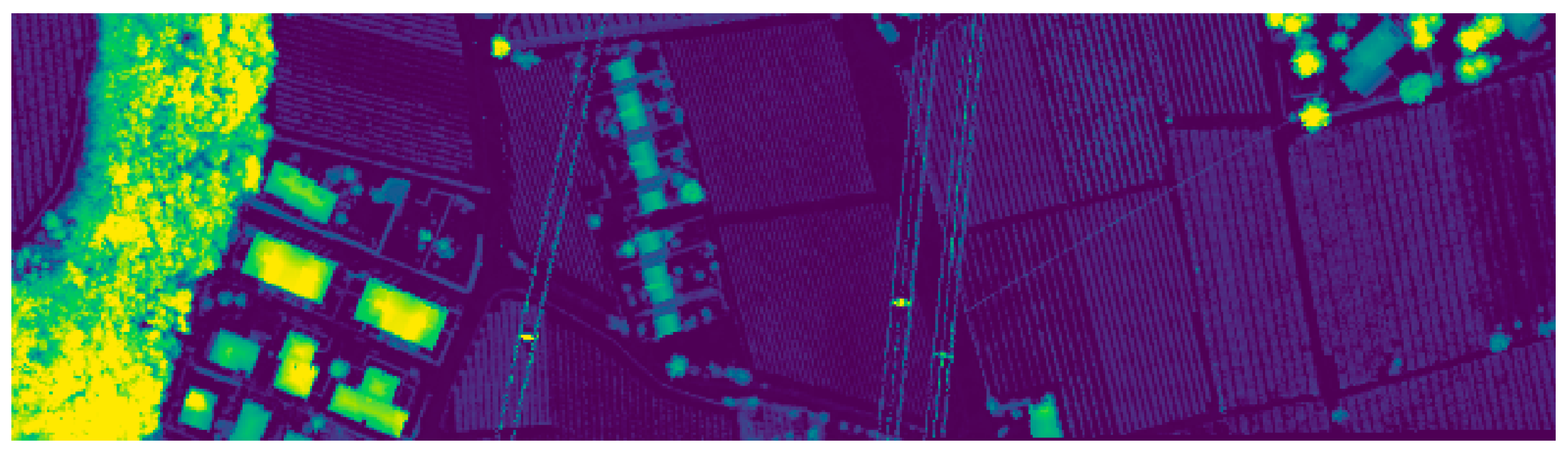
2.1.1. The Trento Dataset

The Trento dataset [31] is an integrated collection of HSI and LiDAR data focused on a rural region in southern Trento, Italy. It incorporates HSI with 63 spectral bands covering wavelengths from 402.89 nm to 989.09 nm, alongside LiDAR data used to generate a Digital Surface Model (DSM). Both the HSI and LiDAR datasets are characterized by a spatial resolution of 1 m and dimensions of 166 × 600 pixels (Figure 1). This dataset includes six well-defined land cover categories, comprising a total of 30,214 sample pixels (

Table 1. Trento dataset.

No.	Class Name	Training	Test	Samples
1	Apple Trees	129	3905	4034
2	Buildings	125	2778	2903
3	Ground	105	374	479
4	Wood	154	8969	9123
5	Vineyard	184	10,317	10,501
6	Roads	122	3052	3174
	Total	819	29,395	30,214

). The hyperspectral data were captured using the AISA Eagle sensor, while LiDAR data acquisition was performed with the Optech ALTM 3100EA system. To ensure precise alignment, these datasets underwent pixel-level registration. The high-resolution nature of this dataset, along with its multimodal integration, provides a significant asset for RS applications, particularly in environmental assessment, precision agriculture, and rural landscape characterization.

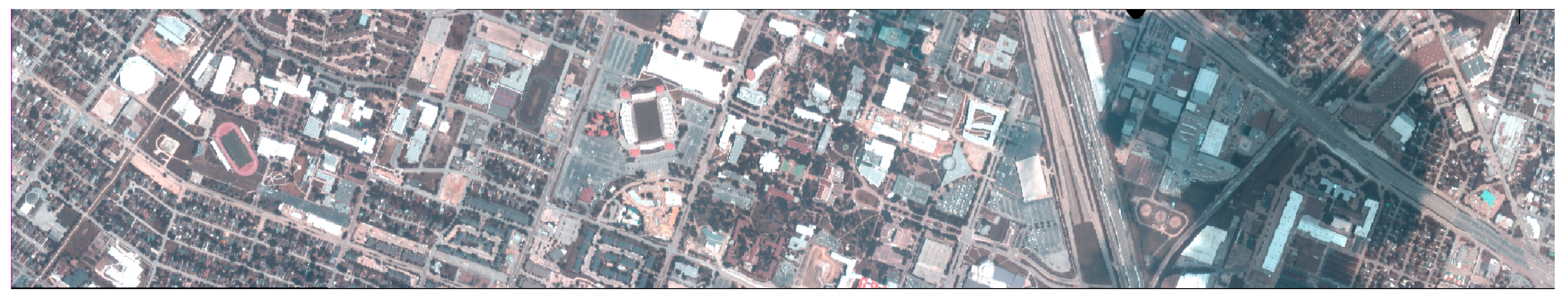
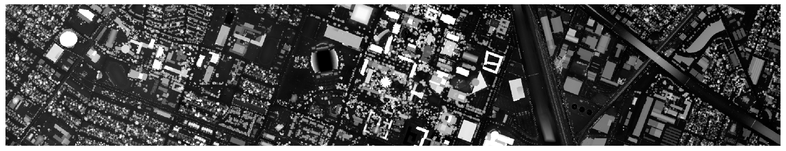
2.1.2. The Houston 2013 Dataset

The Houston 2013 dataset [32] represents a crucial benchmark in the field of RS, encompassing both HSI and LiDAR data collected over the University of Houston campus and adjacent urban regions. This dataset was acquired through an aerial survey conducted by the National Center for Airborne Laser Mapping (NCALM) with financial support from the National Science Foundation (NSF), USA. The hyperspectral component consists of 144 spectral bands, spanning wavelengths from 380 nm to 1050 nm, with a spatial resolution of 2.5 m, covering an area of 349 × 1905 pixels (Figure 2). Meanwhile, the co-registered LiDAR dataset offers detailed elevation insights, complementing the spectral information (Figure 3). Captured on 22–23 June 2012, this dataset serves as a valuable resource for multiple applications, including environmental assessment, urban development planning, and scientific investigations (

Table 2. Houston 2013 dataset.

No.	Class Name	Training	Test	Samples
1	Healthy Grass	198	1053	1251
2	Stressed Grass	190	1064	1254
3	Synthetic Grass	192	505	697
4	Tree	188	1056	1244
5	Soil	186	1056	1242
6	Water	182	143	325
7	Residential	196	1072	1268
8	Commercial	191	1053	1244
9	Road	193	1059	1252
10	Highway	191	1036	1227
11	Railway	181	1054	1235
12	Parking Lot 1	192	1041	1233
13	Parking Lot 2	184	285	469
14	Tennis Court	181	247	428
15	Running Track	187	473	660
	Total	2832	12,197	15,029

), making it particularly useful for advancing RS methodologies.

2.2. Methods

In this section, we present the methodological framework developed for plant classification within wetland ecosystems. This approach is tailored to integrate HSI and LiDAR data, harnessing their complementary attributes to enhance classification accuracy and model robustness. The proposed framework is structured around three key components. These modules operate in a sequential and interdependent manner, facilitating data preprocessing, feature extraction, multimodal fusion, and species classification. A detailed discussion of each module is provided in the subsequent subsections.

2.2.1. Overall Framework

The proposed PlantViT model introduces an innovative framework that leverages attention mechanisms to explore inherent correlations and complementary features within fused HSI and LiDAR multimodal data. By integrating these multimodal datasets, the model effectively captures spatial–spectral dependencies, enhancing classification accuracy and robustness. As shown in Figure 4, PlantViT is built upon the LightViT foundation and is structured into three components: the modules for feature extraction, fusion, and classification. The primary objective of this framework is to handle the cross-modal feature fusion of spectral and spatial channels while incorporating attention mechanisms that focus on both local and global information. Through this design, our framework offers a lightweight solution for the PlantViT model, enabling more efficient identification of vegetation categories with enhanced performance and scalability.

2.2.2. Spectral–Spatial Extractor Module (SSE)

The Spectral–Spatial Extractor Module (SSE) is responsible for extracting meaningful features from both HSI and LiDAR data. This module comprises the following submodules: Feature_HSI, Spectral Weight (implemented using the involution method), Spatial Feature, and Spatial Weight. This integrated approach ensures that spectral and spatial characteristics are optimally utilized, laying a solid foundation for subsequent multimodal fusion and advanced processing tasks. The precise fusion of these features improves both the accuracy and granularity of the combined dataset, enabling more informed analyses and decision making in intricate environmental and geographical contexts.

1.

Feature HSI

The Feature_HSI module extracts spectral–spatial features from the HSI data through sequential convolutional layers, using dynamic kernel generation via the involution mechanism. The process involves matrix multiplication, bias addition, and non-linear activation, as described by the following equation:

$${\mathrm{X}}_{\mathrm{HSI}}^{\left(l+1\right)}=\varphi \left({\mathrm{W}}^{\left(l\right)}\cdot {\mathrm{X}}_{\mathrm{HSI}}^{\left(l\right)}+{\mathrm{b}}^{\left(l\right)}\right)$$

(1)

Here, ${\mathrm{X}}_{\mathrm{HSI}}^{\left(l\right)}$ represents the matrix of input features to layer $l$, ${\mathrm{W}}^{\left(l\right)}$ is the matrix of weights corresponding to the convolution filters (Spectral Weight), and ${\mathrm{b}}^{\left(l\right)}$ is the bias vector. The operation $\cdot$ denotes matrix multiplication, and $\varphi$ represents a non-linear activation function such as ReLU.

The involution operation, which dynamically adjusts the convolutional kernels based on the input features, can be more formally represented as

$${\mathrm{K}}_{\mathrm{HSI}}^{\left(l\right)}={\mathrm{vec}}^{-1}\left({\mathrm{G}}^{\left(l\right)}\left(\varphi \left({\mathrm{F}}^{\left(l\right)}\cdot \mathrm{vec}\left({\mathrm{X}}_{\mathrm{HSI}}^{\left(l\right)}\right)\right)\right)\right)$$

(2)

Here, ${\mathrm{F}}^{\left(l\right)}$ and ${\mathrm{G}}^{\left(l\right)}$ are the matrices that transform the feature space to generate kernel weights. The function $\mathrm{vec}$ vectorizes its matrix argument, and ${\mathrm{vec}}^{-1}$ converts a vector back into a matrix form suitable for convolution. ${\mathrm{K}}_{\mathrm{HSI}}^{\left(l\right)}$ represents the matrix of dynamically adjusted kernel weights. The application of dynamically generated kernels to the input features is captured by

$${\mathrm{Y}}_{\mathrm{HSI}}^{\left(l\right)}={\mathrm{K}}_{\mathrm{HSI}}^{\left(l\right)}\ast {\mathrm{X}}_{\mathrm{HSI}}^{\left(l\right)}$$

(3)

Here, $\ast$ denotes the convolution operation applied using the dynamic kernels ${\mathrm{K}}_{\mathrm{HSI}}^{\left(l\right)}$ on the input feature matrix ${\mathrm{X}}_{\mathrm{HSI}}^{\left(l\right)}$. This operation can be seen as a matrix multiplication where each element of the output matrix ${\mathrm{Y}}_{\mathrm{HSI}}^{\left(l\right)}$ is computed as a weighted sum of local patches of ${\mathrm{X}}_{\mathrm{HSI}}^{\left(l\right)}$, with weights provided by ${\mathrm{K}}_{\mathrm{HSI}}^{\left(l\right)}$.

2.

Feature LiDAR

The LiDAR feature extraction module utilizes a convolutional layer to derive spatial characteristics from LiDAR data. Unlike HSI, LiDAR data do not provide spectral information but focus on capturing spatial structures. The convolutional operation is similar to the HSI extraction:

$${\mathrm{X}}_{\mathrm{LiDAR}}=\varphi \left(\mathrm{W}\cdot {\mathrm{X}}_{\mathrm{LiDAR}}+\mathrm{b}\right)$$

(4)

Here, ${\mathrm{X}}_{\mathrm{LiDAR}}$ represents the matrix of input features, $\mathrm{W}$ is the matrix of weights corresponding to the convolutional filters, and $\mathrm{b}$ is the bias vector. The operation $\cdot$ denotes convolution, and $\varphi$ corresponds to a non-linear activation function, including ReLU.

To further enhance the extracted spatial features from LiDAR, spectral–spatial features from HSI data are integrated dynamically. The joint features of LiDAR and HSI are concatenated to generate context-aware convolutional kernels, formally represented as

$${\mathrm{K}}_{\mathrm{LiDAR}-\mathrm{HSI}}={\mathrm{vec}}^{-1}\left(\mathrm{G}\cdot \left(\varphi \left(\mathrm{F}\cdot \mathrm{vec}\left({\mathrm{X}}_{\mathrm{LiDAR}}{+\mathrm{X}}_{\mathrm{HSI}}\right)\right)\right)\right)$$

(5)

Here, $\mathrm{F}$ and $\mathrm{G}$ are the matrices that transform the joint feature space to generate kernel weights, $+$ combines LiDAR and HSI features along the channel dimension, $\mathrm{vec}\left(\cdot \right)$ vectorizes the joint features, and ${\mathrm{vec}}^{-1}\left(\cdot \right)$ converts a vector back into a matrix suitable for convolution. ${\mathrm{K}}_{\mathrm{LiDAR}-\mathrm{HSI}}$ represents the matrix of dynamically adjusted kernel weights (Spatial Weight).

The dynamically generated kernels are then applied to the input LiDAR features as

$${\mathrm{Y}}_{\mathrm{LiDAR}}^{\left(l\right)}={\mathrm{K}}_{\mathrm{LiDAR}-\mathrm{HSI}}\ast {\mathrm{X}}_{\mathrm{LiDAR}}^{\left(l\right)}$$

(6)

These joint features are processed through dynamic kernels to extract refined spatial features.

2.2.3. Multimodal Fusion Integrator (MFI)

The Multimodal Fusion Integrator (MFI) is responsible for combining features from different data sources, ensuring they are properly aligned for further processing. Initially, each feature set undergoes transformation through a dimension module that standardizes and refines the feature representations:

$${\mathrm{F}}_i^{\left(l\right)}=\varphi \left(\mathrm{BN}\left({\mathrm{W}}_i^{\left(l\right)}\cdot {\mathrm{X}}_i^{\left(l\right)}+{\mathrm{b}}_i^{\left(l\right)}\right)\right)$$

(7)

where ${\mathrm{X}}_i^{\left(l\right)}$ denotes the input features to the $l$ dimension module for the $i$ modality, ${\mathrm{W}}_i^{\left(l\right)}$ and ${\mathrm{b}}_i^{\left(l\right)}$ are the weights and biases of the module, $\cdot$ denotes matrix multiplication, BN represents batch normalization, and $\varphi$ is the ReLU activation function.

After dimension transformation, the features from different sources are concatenated along the feature dimension:

$$\mathrm{Z}=\mathrm{Concat}\left({\mathrm{F}}_1^{\left(l\right)},{\mathrm{F}}_2^{\left(l\right)},\dots ,{\mathrm{F}}_n^{\left(l\right)}\right)$$

(8)

where $\mathrm{Z}$ represents the concatenated feature vector from $n$ different transformed feature sets.

The concatenated features are fused through a weighted sum, employing learnable parameters to balance the contribution of each feature set:

$${\mathrm{F}}_{\mathrm{fused}}={\displaystyle \sum _{i=1}^n{\lambda }_i{\mathrm{Z}}_i}$$

(9)

where ${\lambda }_i$ are learnable weights associated with each feature set ${\mathrm{Z}}_i$, optimized during training to maximize fusion effectiveness.

A transformer-based module (PlantViT) can further process the fused features to capture complex dependencies:

$$\mathrm{Y}=\mathrm{PlantViT}\left({\mathrm{F}}_{\mathrm{fused}}\right)$$

(10)

where $\mathrm{ViT}$ denotes the LightViT operation and $\mathrm{Y}$ represents the output feature map, which combines the local and global context derived from the fused input data.

2.2.4. Deep Feature Classifier (DFC)

The Deep Feature Classifier model utilizes a LightViT-based architecture, adapted for handling complex spatial data such as the data encountered in RS applications. This section thoroughly details the DFC in conjunction with the parameter configurations.

1.

Patch Embedding

The initial step involves transforming the spatial image data into a sequence of flattened patches. The image $X$ with dimensions $C_{in}=8$ channels is partitioned into patches of size $P=2\times 2$, which are then embedded into vectors of dimension $D$, where $D$ changes through the layers [96, 192, 384]:

$$Z_0=\left[X_1^P{W}^E;\dots ;X_N^P{W}^E\right]+B^E$$

(11)

Here, $W^E\in {ℝ}^{\left(P^2·C_{in}\right)\times D}$ is the embedding matrix tailored to the initial dimension $D=96$, and $B^E$ is the corresponding bias. This configuration allows the model to transform raw pixel values into a high-dimensional feature space conducive to the self-attention mechanism.

2.

Positional Encoding

Positional encodings $E_{pos}$ are added to the embedded patches to maintain the spatial context within the sequence. The dimension of $E_{pos}$ matches that of $Z_0=Z_0+E_{pos}$. This addition ensures that despite the transformation, spatial information is preserved and utilized in subsequent layers.

3.

Transformer Blocks

Configured with different layers and heads at each stage ([2, 2, 2] layers and [3, 6, 12] heads), the transformer blocks process the data as follows.

In Multi-Head Self-Attention (MHA), for each $hea{d}_i$ in each layer, the queries $Q$, key $K$, and values $V$ are computed from $Z$ using separate learned matrices for each dimension set:

$$MHA\left(Q,K,V\right)=Concat\left(hea{d}_1,\dots ,hea{d}_h\right)W^O$$

(12)

$$hea{d}_i=soft\max \left({\displaystyle \frac{Q_i{K}_i^T}{\sqrt{d_k}}}\right)V_i$$

(13)

Here, $Q_i=Z{W}_i^Q$, $K_i=Z{W}_i^K$, $V_i=Z{W}_i^V$ for each $hea{d}_i$, and $d_k$ is the dimensionality of the keys. The Feed-Forward Network (FFN) is computed as follows:

$$FFN\left(Z\right)\sigma \left(Z{W}_1+b_1\right)W_2+b_2$$

(14)

where $W_1$, $W_2$ are the weight matrices and $b_1$, $b_2$ as are the biases. The expansion ratios for the FFNs are [8, 4, 4], allowing varying degrees of complexity in the transformations.

4.

Classification

After each sublayer

$$Z=LayerNorm\left(Z+Sublayer\left(Z\right)\right)$$

(15)

These components help stabilize the learning process and promote the integration of features across different layers.

$$Y=Z_L{W}^C+b^C$$

(16)

$$\mathrm{Probabilities}=soft \max \left(Y\right)$$

(17)

where $W^c$ and $b^C$ are the weights and bias of the output projection layer, respectively. This final step converts the complex feature interactions captured by the transformer into actionable class predictions.

3. Experiments and Results

3.1. Experimental Setup

In this section, we outline the setup for the experiments conducted to evaluate the performance of the proposed model. The experiments were performed using two distinct datasets: the Trento dataset and the Houston 2013 dataset. These datasets differ significantly in terms of geographical location, landscape characteristics, and vegetation types, making them suitable for assessing the generalization ability of the model across varied environments. Detailed descriptions of both datasets were provided in Section 2.

3.2. Implementation Details and Evaluation

In this study, we detail the implementation and evaluation of the Fusion model using the PyTorch framework (version 1.11.0), emphasizing our rigorous experimental setup designed to assess its performance across diverse datasets. Below is a consolidated overview of the optimizer, loss function, training parameters, and evaluation metrics used in the experiments.

Data were split into training and testing sets, with the Trento dataset having a smaller proportion of training samples (2.71%) compared to the Houston dataset (18.84%). This setup tests the model’s learning efficiency and generalization capability from limited data.

3.2.1. Model Implementation and Training

To ensure optimal training stability and classification performance, hyperparameters were selected based on prior studies and empirical evaluations.

• Optimizer and learning rate. The Adam optimizer was used for training with a learning rate of 0.01. A comparison among 0.001, 0.005, 0.01, and 0.05 indicated that 0.01 provided the best balance between convergence speed and accuracy. Betas and Epsilon were set to default values, supported by prior studies on ViT in RS.
• Loss function: Soft-Target Cross-Entropy was employed to enhance class separability and mitigate class imbalance, which is common in RS datasets.
• Batch size: A batch size of 32 was chosen, as it balances computational efficiency and generalization ability. Tests with 16, 32, and 64 showed that 32 provided stable gradient updates without excessive memory consumption.
• Number of training epochs: The model was trained for 100 epochs, determined through validation loss convergence analysis. Training with 50 epochs was insufficient, while exceeding 100 epochs led to diminishing returns and increased overfitting risk.
• Regularization techniques: To prevent overfitting, L2 regularization (weight decay = 1 × 10⁻⁴) and Dropout (0.3) were applied in the transformer layers, following best practices in DL.

Overall, the hyperparameter selection was systematically optimized to maximize classification performance while ensuring computational efficiency and model adaptability to varying environmental conditions.

3.2.2. Model Evaluation and Metrics

To assess the effectiveness and robustness of the Fusion model, we employed several key performance metrics:

• Overall accuracy (OA): measures the proportion of correctly predicted observations to the total observations, providing a holistic view of model accuracy.
• Average accuracy (AA): represents the average of accuracies computed for each class, offering insights into class-wise performance.
• Kappa coefficient ($\kappa$): quantifies the agreement of prediction with the true labels, corrected by the randomness of agreement, serving as a robust statistic for classification accuracy.

These evaluation metrics are extracted from the confusion matrix, enabling an in-depth assessment of the model’s classification performance across multiple categories.

The experimental design, model deployment, and validation strategy presented in this study are systematically incorporated to highlight the Fusion model’s enhanced ability to process complex datasets by leveraging HSI and LiDAR data. This comprehensive evaluation not only substantiates the model’s effectiveness in classification but also reinforces its potential applicability in RS and other scientific domains.

3.3. Experimental Results

In this section, we report the Fusion model’s classification performance on both the Trento and Houston 2013 datasets. The evaluation was conducted using multiple metrics, including OA, class-specific accuracy, and $\kappa$, with additional performance indicators to ensure a comprehensive assessment.

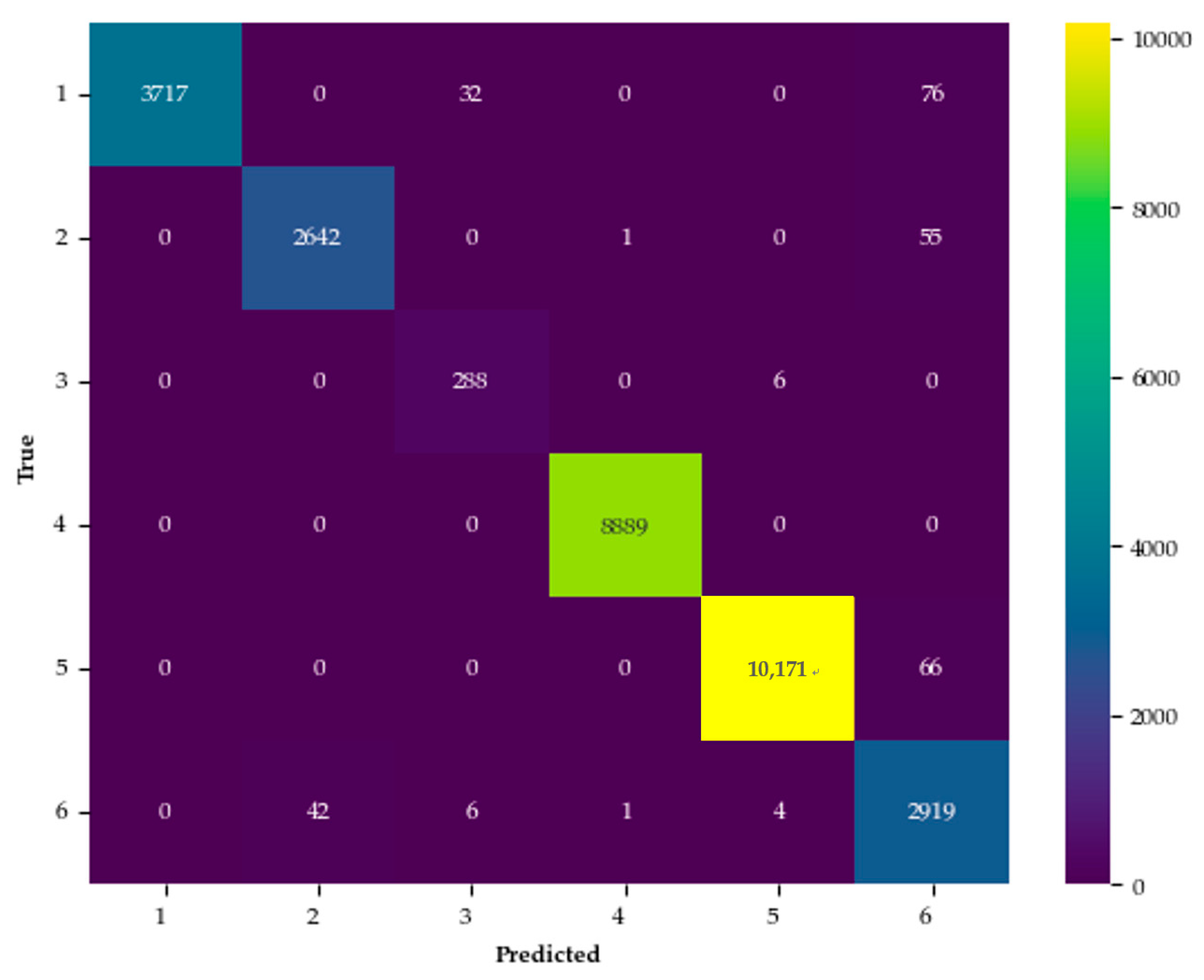
3.3.1. Performance on the Trento Dataset

The Trento dataset, representing natural landscapes in northern Italy, showed excellent performance in vegetation classification. The Fusion model achieved an OA of 99.00%, an AA of 98.44%, and a $\kappa$ of 98.66 (see

Table 3. Performance metrics (in%).

No.	Class Name	Accuracy	Precision	Recall	F1-Score
1	Apple trees	97.18	99.18	97.33	98.25
2	Buildings	97.92	98.23	97.92	98.07
3	Ground	97.96	95.68	97.96	96.81
4	Wood	100.00	99.99	99.99	99.99
5	Vineyard	99.36	99.35	99.35	99.35
6	Roads	98.22	96.82	97.46	97.14
OA					99.00
AA					98.44
$\kappa$					98.66

). The model demonstrated promising results across all vegetation classes, particularly in the Wood class, where it achieved 100% accuracy in both precision and recall. The Vineyard class also showed high accuracy (99.36%), indicating the model’s capability in distinguishing vegetation types with distinct spectral signatures.

Despite the overall high accuracy, the Apple Trees class exhibited slightly lower recall (97.33%) than other classes, likely due to variations in the appearance of the trees under different environmental conditions. Nevertheless, the model’s performance remained strong across the board.

However, such perfect accuracy, especially in the Wood class, raises concerns about potential overfitting. Achieving 100% accuracy in real-world RS applications is rare. Although overfitting concerns exist, it is important to note that steps such as regularization techniques were applied to mitigate these risks, as discussed in earlier sections. These measures help ensure that the model’s performance is not over-optimized for a specific dataset, thereby improving its generalization ability.

To further assess the model’s classification performance, we present the confusion matrix for the Trento dataset (Figure 5). The matrix highlights the model’s ability to correctly classify most vegetation classes, with a minimal number of misclassifications. Notably, the Wood and Vineyard classes exhibited near-perfect classification, confirming the model’s effectiveness in these categories. The confusion matrix also reveals slight misclassifications in Apple Trees, but overall, the results demonstrate the model’s strong ability to differentiate between vegetation classes.

3.3.2. Performance on the Houston 2013 Dataset

The Houston 2013 dataset, which includes a mixture of urban and natural land cover types, presented a more complex classification task. Despite this, the Fusion model achieved an OA of 97.41%, an AA of 97.59%, and a $\kappa$ of 97.19 (see

Table 4. Classification performance by class (in%).

No.	Class Name	Accuracy	Precision	Recall	F1-Score
1	Healthy Grass	97.15	97.00	98.00	98.00
2	Stressed Grass	97.46	97.00	98.00	98.00
3	Synthetic Grass	99.80	99.00	99.00	99.00
4	Trees	95.55	100.00	98.00	97.00
5	Soil	100.00	100.00	100.00	100.00
6	Water	97.20	97.00	98.00	98.00
7	Residential	92.82	97.00	95.00	94.00
8	Commercial	96.39	96.00	96.00	95.00
9	Road	97.92	98.00	97.00	97.00
10	Highway	100.00	100.00	100.00	100.00
11	Railway	96.39	97.00	96.00	95.00
12	Parking Lot 1	99.62	100.00	99.00	99.00
13	Parking Lot 2	98.60	100.00	99.00	99.00
14	Tennis Court	100.00	100.00	100.00	100.00
15	Running Track	94.93	95.00	96.00	94.00
OA					97.41
AA					97.59
$\kappa$					97.19

). The model achieved high classification accuracy across various vegetation categories, including Healthy Grass (97.15%) and Stressed Grass (97.46%), exhibiting precision and recall values.

However, the classification accuracy for the Trees category was slightly lower at 95.55%, likely due to spectral similarities with nearby urban structures. Similarly, the Residential class showed a marginally reduced accuracy of 92.82%, potentially influenced by the spectral mixing of vegetation and built-up areas. Despite these challenges, the model maintained robust performance in vegetation classification, even within complex urban landscapes.

The confusion matrix for the Houston 2013 dataset (Figure 6) offers a comprehensive analysis of the classification outcomes. The results indicate high accuracy in vegetation-related categories, including Healthy Grass, Synthetic Grass, and Soil. However, some misclassification was observed between Trees and Urban classes, particularly in areas with complex spectral characteristics. This finding highlights the inherent challenge of vegetation classification in urban environments while also showcasing the model’s ability to effectively distinguish diverse land cover types.

4. Discussion

In this section, we compare the performance of the proposed PlantViT model with other approaches across two benchmark datasets: Trento and Houston 2013. The objective is to assess PlantViT’s effectiveness in vegetation classification and examine its advantages in adapting to diverse geographical landscapes and varied land cover types.

4.1. Performance Comparison on the Trento Dataset

As shown in

Table 5. Accuracy of classification (%) on the Trento dataset.

No.	Class Name	PlantViT	EndNet [33]	DCT [16]	MBF [34]	AM3Net [35]	HES2T [36]	BTRF [37]	TTCNN [38]
1	Apple Trees	97.18	88.19	99.13	98.71	97.12	99.46	95.92	98.07
2	Buildings	97.92	98.49	99.44	98.87	96.73	91.65	98.04	95.21
3	Ground	97.96	95.19	99.94	97.79	98.96	87.43	80.33	93.32
4	Wood	100.00	99.30	92.76	99.89	99.12	98.33	99.83	99.93
5	Vineyard	99.36	91.96	86.37	99.25	98.22	97.65	99.29	98.78
6	Roads	98.22	90.14	92.78	92.38	93.76	68.94	97.66	89.98
	OA	99.00	94.17	97.45	98.62	97.75	94.42	98.66	97.92
	AA	98.44	93.88	95.07	98.14	97.32	90.58	95.30	96.19
	$\kappa$	98.66	92.22	96.58	97.81	97.00	92.54	98.20	96.81

, the PlantViT model outperforms all other models in terms of OA, AA, and $\kappa$ on the Trento dataset. The OA of 99.00% achieved by PlantViT is substantially higher than that of the other models, with EndNet achieving 94.17% and DCT reaching 97.45%. This result highlights the robustness of PlantViT in accurately classifying natural landscape features, including diverse vegetation types such as Apple Trees, Vineyards, and Woods. In particular, PlantViT excels in the classification of challenging classes such as “Apple Trees” (97.18% accuracy). On the other hand, some models like DCT and MBF show lower performance on these classes, underscoring the advantages of using DL-based feature fusion and classification approaches like PlantViT. Additionally, the $\kappa$ of 98.66% confirms the high level of agreement between predicted and true labels, reinforcing the model’s strong classification reliability.

4.2. Performance Comparison on the Houston 2013 Dataset

The results for the Houston 2013 dataset in

Table 6. Accuracy of classification (%) on the Houston 2013 dataset.

No.	Class Name	PlantViT	MSST [39]	mFormer [40]	S2CA [41]	RFFT [42]	MATA [43]	CSF [44]	SFE-FN [22]
1	Healthy Grass	97.15	89.12	82.37	84.62	87.96	91.64	82.72	95.06
2	Stressed Grass	97.46	92.85	85.03	95.68	95.90	83.83	82.24	96.52
3	Synthetic Grass	99.80	95.43	98.09	100.00	97.41	100.00	100.00	100.00
4	Trees	95.55	91.13	95.23	99.62	97.74	99.24	92.52	100.00
5	Soil	100.00	100.00	99.15	100.00	95.32	99.34	98.67	99.81
6	Water	97.20	86.31	98.14	100.00	97.84	100.00	95.10	97.20
7	Residential	92.82	72.35	89.61	87.03	92.57	85.91	80.97	93.00
8	Commercial	96.39	76.87	72.33	93.02	95.42	94.59	81.67	88.98
9	Road	97.92	79.40	88.86	89.71	91.74	91.78	86.87	87.44
10	Highway	100.00	99.57	61.97	71.43	99.10	91.12	79.63	98.17
11	Railway	96.39	98.06	96.24	98.96	96.86	97.91	83.30	93.55
12	Parking Lot 1	99.62	98.09	94.46	98.94	94.56	95.39	88.95	96.35
13	Parking Lot 2	98.60	80.35	87.02	85.67	95.30	92.98	87.37	81.40
14	Tennis Court	100.00	100.00	99.73	91.90	93.22	100.00	100.00	100.00
15	Running Track	94.93	100.00	96.69	100.00	97.57	100.00	99.52	100.00
	OA	97.41	90.29	87.85	92.52	95.01	93.83	89.42	95.11
	AA	97.59	90.63	89.66	93.11	95.23	94.92	89.24	95.17
	$\kappa$	97.19	89.50	86.81	92.52	94.60	93.31	88.51	94.68

show that PlantViT maintains its superiority over other models across various metrics. Specifically, PlantViT achieves an OA of 97.41%, which is substantially higher than the second-best model, MSST (90.29%), and the other models such as mFormer (87.85%) and RFFT (92.52%). These results demonstrate PlantViT’s effectiveness in urban landscape classification, where the task is more complex due to the mixture of vegetation and man-made structures.

Notably, PlantViT presents promising result in classifying “Synthetic Grass” (99.80%), “Soil” (100%), and “Tennis Court” (100%), where it surpasses other models by a significant margin. The model’s performance on urban classes like “Road” (97.92%), “Residential” (92.82%), and “Commercial” (96.39%) further confirms its adaptability to both natural and urban environments. In contrast, other models struggle with accuracy in these classes, particularly “Residential” and “Road”, where PlantViT’s more robust feature extraction and classification strategies help in achieving higher accuracy.

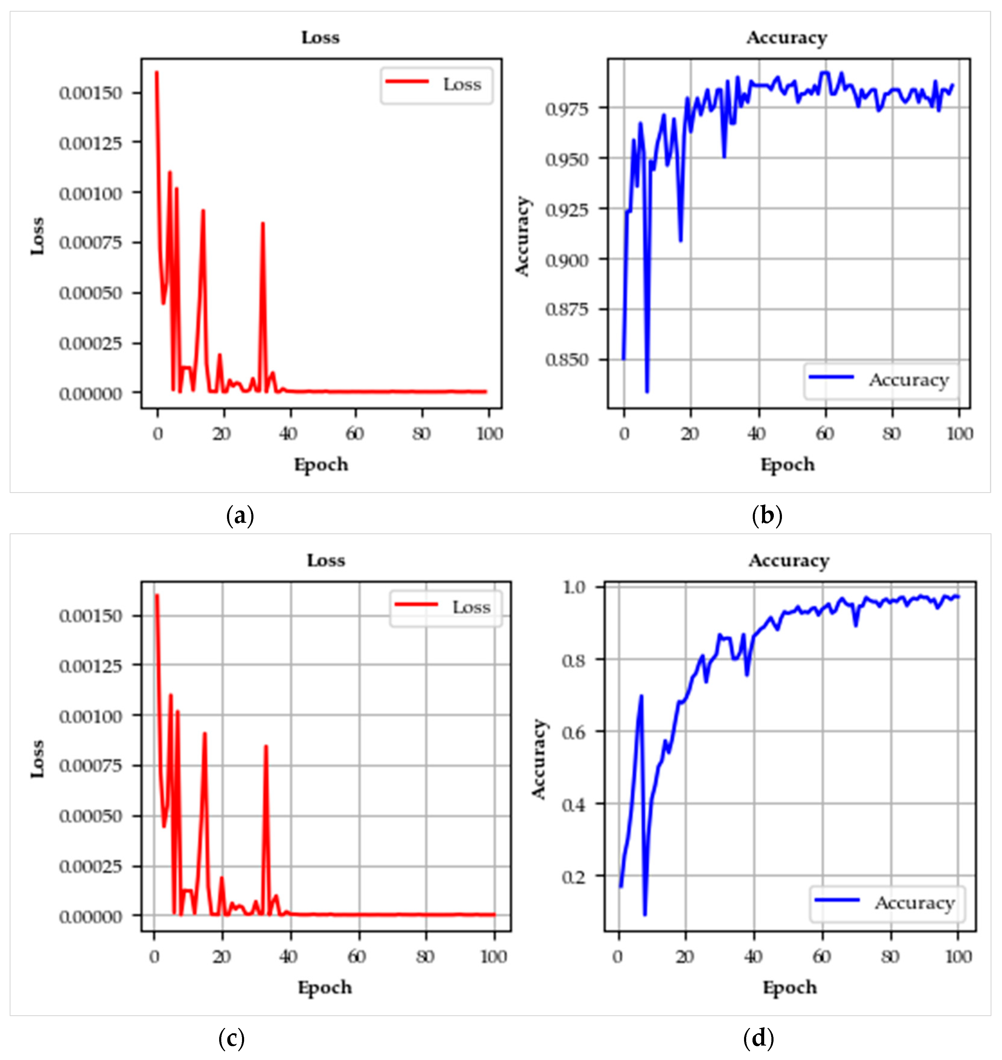
4.3. Learning Curve Insights

The learning curves derived from the Trento and Houston 2013 datasets demonstrate the steady and efficient convergence of PlantViT (Figure 7). In both cases, the training and validation loss decrease steadily across epochs, with minimal signs of overfitting, which suggests that the model is well-regularized and able to generalize effectively. For the Trento dataset, the model reaches near-optimal classification accuracy after relatively few epochs, confirming its ability to learn from limited training data. Similarly, for the Houston 2013 dataset, the learning curves show consistent performance improvement, indicating that PlantViT can adapt to more complex and diverse environments.

4.4. Model Strengths and Advantages

The strong performance of PlantViT can be attributed to several fundamental aspects.

• The integration of high-resolution HSI and LiDAR data enables PlantViT to effectively combine spectral and spatial features, which are essential for accurate vegetation and land cover classification. With its multimodal fusion capability, the model excels in detecting fine-scale landscape features, making it particularly advantageous for monitoring both urban and natural ecosystems.
• Advanced DL architecture: The incorporation of LightViT, a lightweight Vision Transformer, significantly enhances computational efficiency while preserving high classification accuracy. By selectively focusing on the most relevant features within the dataset, LightViT minimizes the need for overly complex network architectures and excessive computational resources, ensuring scalability for large-scale applications.
• Generalization across datasets: The consistent performance of PlantViT on both the Trento and Houston 2013 datasets highlights its robustness and adaptability across different geographical regions and land cover types. This strong generalization capability makes it well-suited for large-scale RS tasks, including vegetation analysis and land-use mapping.

4.5. Conclusion of Comparative Performance

The evaluation results from both datasets confirm that PlantViT surpasses existing models in various vegetation classification tasks. Its consistently strong performance across multiple metrics (e.g., OA, AA, and$\kappa$) on both natural and urban landscapes highlights its practical value in RS applications. The fusion of HSI and LiDAR data, coupled with the efficiency of its lightweight transformer architecture, offers a competitive edge in terms of both classification accuracy and computational efficiency.

In conclusion, PlantViT exhibits substantial potential for large-scale vegetation analysis, environmental assessment, and other RS-driven applications, making it a valuable tool for diverse geographical and ecological contexts.

5. Conclusions

The proposed PlantViT model in this study integrates HSI and LiDAR datasets to improve plant monitoring accuracy. The model addresses critical scientific challenges in plant classification, particularly the issue of cross-environment adaptability and the limitations of traditional DL approaches. The following points summarize the key contributions and innovations of this research:

• Cross-environment adaptability. By integrating HSI and LiDAR data, the model effectively enhances its generalization capability across diverse environmental conditions. Utilizing multiple datasets, including the Trento and Houston 2013 datasets, we demonstrated its adaptability across distinct geographical regions and plant communities. This advancement directly addresses a well-documented challenge in RS—ensuring classification accuracy across heterogeneous ecosystems.
• Overcoming CNN limitations in complex environments. Traditional convolutional neural networks (CNNs) often encounter difficulties in extracting fine-grained spatial–spectral features within intricate plant environments. To mitigate this issue, we incorporated involution-based operations, enabling the model to efficiently capture subtle feature variations while reducing the computational burden typically associated with CNN-based approaches. This enhancement is particularly advantageous for distinguishing morphologically similar plant species within highly heterogeneous landscapes.
• Cross-environment attention mechanism. The fusion of involution with LightViT introduces an innovative attention mechanism that dynamically adjusts to varying environmental contexts. This mechanism enables the model to selectively focus on the most relevant plant features, thereby improving classification robustness and accuracy across diverse ecosystems.

While the PlantViT model demonstrated strong performance across both natural and urban datasets, there are some limitations to be acknowledged.

Although the model showed high classification accuracy in the test datasets, its performance might be constrained by the availability and diversity of training data. Expanding the dataset to include more varied environmental conditions and plant species would likely improve model robustness and generalizability.

The integration of multiple data types (HSI and LiDAR) along with the use of advanced transformers and involution techniques increases model complexity, which may present challenges in terms of computational cost and real-time deployment in large-scale monitoring systems. The future directions of this approach are as follows:

• Future work will involve evaluating the model on additional RS datasets to further assess its robustness and applicability to broader ecological and environmental monitoring tasks.
• Investigating the potential of transfer learning across diverse ecosystems could further enhance the model’s adaptability and generalization capabilities.
• Future research should explore the feasibility of deploying this model in real-time large-scale wetland monitoring. Additionally, incorporating supplementary data sources, such as UAV-based RGB imagery and satellite observations, could expand its practical applications and operational scalability.

Implications for RS applications: The proposed PlantViT model has significant implications for RS, particularly in wetland management and invasive species monitoring. Its ability to combine multiple data modalities and its improved adaptability to varying environmental conditions make it a valuable tool for large-scale, accurate monitoring of plant biodiversity and ecosystem health. By enabling more precise detection of invasive species, this model supports better-informed conservation efforts and management strategies for protecting wetlands and other sensitive ecosystems.

References

1. Ma, Y.; Zhao, Y.; Im, J.; Zhao, Y.; Zhen, Z. A Deep-Learning-Based Tree Species Classification for Natural Secondary Forests Using Unmanned Aerial Vehicle Hyperspectral Images and LiDAR. Ecol. Indic. 2024, 159, 111608. [Google Scholar] [CrossRef]
2. Shi, Y.; Wang, T.; Skidmore, A.K.; Holzwarth, S.; Heiden, U.; Heurich, M. Mapping Individual Silver Fir Trees Using Hyperspectral and LiDAR Data in a Central European Mixed Forest. Int. J. Appl. Earth Obs. Geoinf. 2021, 98, 102311. [Google Scholar] [CrossRef]
3. de Almeida, D.R.A.; Broadbent, E.N.; Ferreira, M.P.; Meli, P.; Zambrano, A.M.A.; Gorgens, E.B.; Resende, A.F.; de Almeida, C.T.; do Amaral, C.H.; Corte, A.P.D.; et al. Monitoring Restored Tropical Forest Diversity and Structure through UAV-Borne Hyperspectral and Lidar Fusion. Remote Sens. Environ. 2021, 264, 112582. [Google Scholar] [CrossRef]
4. Mohan, M.; Richardson, G.; Gopan, G.; Aghai, M.M.; Bajaj, S.; Galgamuwa, G.A.P.; Vastaranta, M.; Arachchige, P.S.P.; Amorós, L.; Corte, A.P.D.; et al. UAV-Supported Forest Regeneration: Current Trends, Challenges and Implications. Remote Sens. 2021, 13, 2596. [Google Scholar] [CrossRef]
5. Guo, F.; Li, Z.; Meng, Q.; Ren, G.; Wang, L.; Wang, J.; Qin, H.; Zhang, J. Semi-Supervised Cross-Domain Feature Fusion Classification Network for Coastal Wetland Classification with Hyperspectral and LiDAR Data. Int. J. Appl. Earth Obs. Geoinf. 2023, 120, 103354. [Google Scholar] [CrossRef]
6. Baena, S.; Moat, J.; Whaley, O.; Boyd, D.S. Identifying Species from the Air: UAVs and the Very High Resolution Challenge for Plant Conservation. PLoS ONE 2017, 12, e0188714. [Google Scholar] [CrossRef]
7. Roy, S.K.; Deria, A.; Hong, D.; Rasti, B.; Plaza, A.; Chanussot, J. Multimodal Fusion Transformer for Remote Sensing Image Classification. IEEE Trans. Geosci. Remote Sens. 2023, 61, 5515620. [Google Scholar] [CrossRef]
8. Wang, R.; Ma, L.; He, G.; Johnson, B.A.; Yan, Z.; Chang, M.; Liang, Y. Transformers for Remote Sensing: A Systematic Review and Analysis. Sensors 2024, 24, 3495. [Google Scholar] [CrossRef]
9. Asner, G.P.; Ustin, S.L.; Townsend, P.; Martin, R.E. Forest Biophysical and Biochemical Properties from Hyperspectral and LiDAR Remote Sensing. In Remote Sensing Handbook, Volume IV; CRC Press: Boca Raton, FL, USA, 2024; ISBN 978-1-003-54117-2. [Google Scholar]
10. Adegun, A.A.; Viriri, S.; Tapamo, J.-R. Review of Deep Learning Methods for Remote Sensing Satellite Images Classification: Experimental Survey and Comparative Analysis. J. Big Data 2023, 10, 93. [Google Scholar] [CrossRef]
11. Dao, P.D.; Axiotis, A.; He, Y. Mapping Native and Invasive Grassland Species and Characterizing Topography-Driven Species Dynamics Using High Spatial Resolution Hyperspectral Imagery. Int. J. Appl. Earth Obs. Geoinf. 2021, 104, 102542. [Google Scholar] [CrossRef]
12. Li, Q.; Wong, F.K.K.; Fung, T. Mapping Multi-Layered Mangroves from Multispectral, Hyperspectral, and LiDAR Data. Remote Sens. Environ. 2021, 258, 112403. [Google Scholar] [CrossRef]
13. Yang, C. Remote Sensing and Precision Agriculture Technologies for Crop Disease Detection and Management with a Practical Application Example. Engineering 2020, 6, 528–532. [Google Scholar] [CrossRef]
14. Esmaeili, M.; Abbasi-Moghadam, D.; Sharifi, A.; Tariq, A.; Li, Q. ResMorCNN Model: Hyperspectral Images Classification Using Residual-Injection Morphological Features and 3DCNN Layers. IEEE J. Sel. Top. Appl. Earth Obs. Remote Sens. 2024, 17, 219–243. [Google Scholar] [CrossRef]
15. Norton, C.L.; Hartfield, K.; Collins, C.D.H.; van Leeuwen, W.J.D.; Metz, L.J. Multi-Temporal LiDAR and Hyperspectral Data Fusion for Classification of Semi-Arid Woody Cover Species. Remote Sens. 2022, 14, 2896. [Google Scholar] [CrossRef]
16. Dang, Y.; Zhang, X.; Zhao, H.; Liu, B. DCTransformer: A Channel Attention Combined Discrete Cosine Transform to Extract Spatial–Spectral Feature for Hyperspectral Image Classification. Appl. Sci. 2024, 14, 1701. [Google Scholar] [CrossRef]
17. Kuras, A.; Brell, M.; Rizzi, J.; Burud, I. Hyperspectral and Lidar Data Applied to the Urban Land Cover Machine Learning and Neural-Network-Based Classification: A Review. Remote Sens. 2021, 13, 3393. [Google Scholar] [CrossRef]
18. Zhang, M.; Li, W.; Zhang, Y.; Tao, R.; Du, Q. Hyperspectral and LiDAR Data Classification Based on Structural Optimization Transmission. IEEE Trans. Cybern. 2023, 53, 3153–3164. [Google Scholar] [CrossRef]
19. Kashefi, R.; Barekatain, L.; Sabokrou, M.; Aghaeipoor, F. Explainability of Vision Transformers: A Comprehensive Review and New Perspectives. arXiv 2023, arXiv:2311.06786. [Google Scholar]
20. Lecun, Y.; Bottou, L.; Bengio, Y.; Haffner, P. Gradient-Based Learning Applied to Document Recognition. Proc. IEEE 1998, 86, 2278–2324. [Google Scholar] [CrossRef]
21. Li, J.; Hong, D.; Gao, L.; Yao, J.; Zheng, K.; Zhang, B.; Chanussot, J. Deep Learning in Multimodal Remote Sensing Data Fusion: A Comprehensive Review. Int. J. Appl. Earth Obs. Geoinf. 2022, 112, 102926. [Google Scholar] [CrossRef]
22. Shen, X.; Deng, X.; Geng, J.; Jiang, W. SFE-FN: A Shuffle Feature Enhancement-Based Fusion Network for Hyperspectral and LiDAR Classification. IEEE Geosci. Remote Sens. Lett. 2023, 20, 5501605. [Google Scholar] [CrossRef]
23. Shi, Y.; Skidmore, A.K.; Wang, T.; Holzwarth, S.; Heiden, U.; Pinnel, N.; Zhu, X.; Heurich, M. Tree Species Classification Using Plant Functional Traits from LiDAR and Hyperspectral Data. Int. J. Appl. Earth Obs. Geoinf. 2018, 73, 207–219. [Google Scholar] [CrossRef]
24. Zhang, Z.; Zhu, L. A Review on Unmanned Aerial Vehicle Remote Sensing: Platforms, Sensors, Data Processing Methods, and Applications. Drones 2023, 7, 398. [Google Scholar] [CrossRef]
25. Ding, J.; Ren, X.; Luo, R. An Adaptive Learning Method for Solving the Extreme Learning Rate Problem of Transformer. In Proceedings of the Natural Language Processing and Chinese Computing; Liu, F., Duan, N., Xu, Q., Hong, Y., Eds.; Springer: Cham, Switzerland, 2023; pp. 361–372. [Google Scholar]
26. Tusa, E.; Laybros, A.; Monnet, J.-M.; Dalla Mura, M.; Barré, J.-B.; Vincent, G.; Dalponte, M.; Féret, J.-B.; Chanussot, J. Chapter 2.11—Fusion of Hyperspectral Imaging and LiDAR for Forest Monitoring. In Data Handling in Science and Technology; Amigo, J.M., Ed.; Hyperspectral Imaging; Elsevier: Amsterdam, The Netherlands, 2019; Volume 32, pp. 281–303. [Google Scholar]
27. Huang, T.; Huang, L.; You, S.; Wang, F.; Qian, C.; Xu, C. LightViT: Towards Light-Weight Convolution-Free Vision Transformers. arXiv 2022, arXiv:2207.05557. [Google Scholar]
28. Wäldchen, J.; Rzanny, M.; Seeland, M.; Mäder, P. Automated Plant Species Identification—Trends and Future Directions. PLoS Comput. Biol. 2018, 14, e1005993. [Google Scholar] [CrossRef]
29. Ding, M.; Xiao, B.; Codella, N.; Luo, P.; Wang, J.; Yuan, L. DaViT: Dual Attention Vision Transformers. In Proceedings of the Computer Vision—ECCV 2022, Tel Aviv, Israel, 23–27 October 2022; Avidan, S., Brostow, G., Cissé, M., Farinella, G.M., Hassner, T., Eds.; Springer: Cham, Switzerland, 2022; pp. 74–92. [Google Scholar]
30. Li, D.; Hu, J.; Wang, C.; Li, X.; She, Q.; Zhu, L.; Zhang, T.; Chen, Q. Involution: Inverting the Inherence of Convolution for Visual Recognition. arXiv 2021, arXiv:2103.06255. [Google Scholar]
31. Available online: https://github.com/shuxquan/PlantViT/tree/main/trento (accessed on 30 March 2025).
32. Available online: https://github.com/shuxquan/PlantViT/tree/main/Houston%202013 (accessed on 30 March 2025).
33. Hong, D.; Gao, L.; Hang, R.; Zhang, B.; Chanussot, J. Deep Encoder–Decoder Networks for Classification of Hyperspectral and LiDAR Data. IEEE Geosci. Remote Sens. Lett. 2022, 19, 5500205. [Google Scholar] [CrossRef]
34. Wang, J.; Tan, X. Mutually Beneficial Transformer for Multimodal Data Fusion. IEEE Trans. Circuits Syst. Video Technol. 2023, 33, 7466–7479. [Google Scholar] [CrossRef]
35. Wang, J.; Li, J.; Shi, Y.; Lai, J.; Tan, X. AM3Net: Adaptive Mutual-Learning-Based Multimodal Data Fusion Network. IEEE Trans. Circuits Syst. Video Technol. 2022, 32, 5411–5426. [Google Scholar] [CrossRef]
36. Wang, W.; Liu, L.; Zhang, T.; Shen, J.; Wang, J.; Li, J. Hyper-ES2T: Efficient Spatial–Spectral Transformer for the Classification of Hyperspectral Remote Sensing Images. Int. J. Appl. Earth Obs. Geoinf. 2022, 113, 103005. [Google Scholar] [CrossRef]
37. Song, T.; Zeng, Z.; Gao, C.; Chen, H.; Li, J. Joint Classification of Hyperspectral and LiDAR Data Using Height Information Guided Hierarchical Fusion-and-Separation Network. IEEE Trans. Geosci. Remote Sens. 2024, 62, 5505315. [Google Scholar] [CrossRef]
38. Xu, X.; Li, W.; Ran, Q.; Du, Q.; Gao, L.; Zhang, B. Multisource Remote Sensing Data Classification Based on Convolutional Neural Network. IEEE Trans. Geosci. Remote Sens. 2018, 56, 937–949. [Google Scholar] [CrossRef]
39. Ma, Y.; Lan, Y.; Xie, Y.; Yu, L.; Chen, C.; Wu, Y.; Dai, X. A Spatial–Spectral Transformer for Hyperspectral Image Classification Based on Global Dependencies of Multi-Scale Features. Remote Sens. 2024, 16, 404. [Google Scholar] [CrossRef]
40. Roy, S.K.; Deria, A.; Shah, C.; Haut, J.M.; Du, Q.; Plaza, A. Spectral–Spatial Morphological Attention Transformer for Hyperspectral Image Classification. IEEE Trans. Geosci. Remote Sens. 2023, 61, 5503615. [Google Scholar] [CrossRef]
41. Wang, X.; Zhu, J.; Feng, Y.; Wang, L. MS2CANet: Multiscale Spatial–Spectral Cross-Modal Attention Network for Hyperspectral Image and LiDAR Classification. IEEE Geosci. Remote Sens. Lett. 2024, 21, 5501505. [Google Scholar] [CrossRef]
42. Shen, X.; Zhu, H.; Meng, C. Refined Feature Fusion-Based Transformer Network for Hyperspectral and LiDAR Classification. In Proceedings of the 2023 International Conference on Image Processing, Computer Vision and Machine Learning (ICICML), Chengdu, China, 3–5 November 2023; pp. 789–793. [Google Scholar]
43. Liu, H.; Li, W.; Xia, X.-G.; Zhang, M.; Tao, R. Multiarea Target Attention for Hyperspectral Image Classification. IEEE Trans. Geosci. Remote Sens. 2023, 61, 5524916. [Google Scholar] [CrossRef]
44. Sun, Y.; Wang, Z.; Li, A.; Jiang, H. Cross-Stage Fusion Network Based Multi-Modal Hyperspectral Image Classification. In Proceedings of the 6GN for Future Wireless Networks, Shanghai, China, 7–8 October 2023; Li, A., Shi, Y., Xi, L., Eds.; Springer Nature Switzerland: Cham, Switzerland, 2023; pp. 77–88. [Google Scholar]
Figure 1. Light Detection and Ranging (LiDAR) Data for Trento dataset.
Forests 16 00620 g001
Figure 2. Hyperspectral imaging (HSI) for Houston 2013 dataset.
Forests 16 00620 g002
Figure 3. LiDAR data for Houston 2013 dataset.
Forests 16 00620 g003
Figure 4. Illustration to clarify the network architecture of the proposed PlantViT for multimodal RS data classification [27,30].
Forests 16 00620 g004
Figure 5. Confusion matrix for Trento dataset.
Forests 16 00620 g005
Figure 6. Confusion matrix for Houston 2013 dataset.
Forests 16 00620 g006
Figure 7. Learning curves: (a,c) the learning curve for loss during the training and validation phases on the Trento and Houston 2013 datasets; (b,d) the learning curve for accuracy during the training and validation phases on the Trento and Houston 2013 datasets.
Forests 16 00620 g007