Article

Enhanced Climate-Sensitive Crop Planning Models for Multiple Criteria Decision-Making When Managing Jack Pine and Red Pine Forest Types

Great Lakes Forestry Centre, Canadian Forest Service, Natural Resources Canada, 1219 Queen Street, Sault Sainte Marie, ON P6A 2E5, Canada
Forests 2025, 16(4), 610; https://doi.org/10.3390/f16040610
Submission received: 11 February 2025 / Revised: 20 March 2025 / Accepted: 26 March 2025 / Published: 30 March 2025
(This article belongs to the Section Wood Science and Forest Products)

Abstract

:
For jack pine (Pinus banksiana Lamb.) and red pine (Pinus resinosa Aiton) forest types, the goal of this study was to develop and demonstrate enhanced climate-smart crop planning models that are capable of simultaneously addressing both conventional and evolving forest management objectives, i.e., volumetric yield, wood quality, carbon storage-based harvestable wood product (HWP) production, and biodiversity-driven deadwood accumulation objectives. Procedurally, this involved the following: (1) development and integration of species-specific cambial age prediction equations and associated integration of whole-stem fibre attribute prediction equation suites, previously developed for wood density (Wd), microfibril angle (Ma), modulus of elasticity (Me), fibre coarseness (Co), tracheid wall thickness (Wt), tracheid radial (Dr) and tangential (Dt) diameters, and specific surface area (Sa), into climate-sensitive structural stand density management models (SSDMMs); (2) modification of the computational pathway of the SSDMMs to enable the estimation of abiotic stem volume production; and (3) given (1) and (2), exemplifying the potential utility of the enhanced SSDMMs in operational crop planning. Analytically, to generate whole-stem attribute predictions and derive HWP estimates, species-specific hierarchical mixed-effects cambial age models were specified, parameterized, and statistically validated. The previously developed attribute equation suites along with the new cambial age models were then integrated within the species-specific SSDMMs. In order to facilitate the calculation of accumulated deadwood production arising from density-dependent (self-thinning) and density-independent (non-self-thinning) mortality, the computational pathways of the SSDMMs were augmented and modified. The utility of the resultant enhanced SSDMMs was then exemplified by generating and contrasting rotational volumetric yield, wood quality attribute property maps, quantity and quality (grade) of solid wood and non-solid wood HWPs, and deadwood production forecasts, for species–locale–RCP-specific crop plan sets. These analytical model-based innovations, along with the crop planning exemplifications, confirmed the adaptability and potential utility of the enhanced SSDMMs in mitigating the complexities of multiple criteria decision-making when managing jack pine and red pine forest types under climate change.

1. Introduction

Realizing traditional volumetric production, economic worth, and ecosystem service objectives while also accommodating (1) biodiversity, wildlife habitat, and wildfire mitigation goals, (2) adhering to regulatory constraints, and (3) accounting for climate change effects, reflects the complexity and multifaceted nature of boreal crop planning. Furthermore, increasing the production of long-lived harvested wood products (HWPs) in order to enhance long-term carbon storage (carbon retainment) and displace fossil fuel-derived construction materials (material substitution) is viewed as an important resource management opportunity, particularly within the context of natural-based climate change mitigation strategies (sensu [1]). Controlling abiotic mass production in order to elicit a reduction in decay-generated carbon emissions and mitigate wildfire risk while simultaneously attaining abiotic mass requirements for biodiversity maintenance is also an evolving management consideration when crop planning.
Although recent advancements in climate-sensitive structural stand density management models (SSDMMs) have improved the prediction of volumetric yield and wood quality outcomes for Canadian conifers when crop planning [2], they lack the ability to forecast HWP production and deadwood accumulation. Recognition of these analytical shortcomings has recently led to renewed efforts to develop more comprehensive forecasting and decision-support models that are capable of addressing these objectives [3]. More generally, the development and subsequent integration of fibre attribute prediction equation suites within existing tree-level and stand-level decision-support crop planning models have been advanced not only in Canada but also in Europe. These latter efforts have included the hybrid process-based growth and yield tree-level models developed for Scots pine (Pinus sylvestris L.) and Norway spruce (Picea abies (L.) Karst.) [4]. Canadian efforts have included the hybrid average-tree and stand-level distance-independent size distribution yield models developed for jack pine (Pinus banksiana Lamb.), black spruce (Picea mariana (Mill) BSP), and red pine (Pinus resinosa Aiton) [5,6].
The approach used in the development of these Canadian models was one of adaption, i.e., incorporating a suite of spatially invariant hierarchical mixed-effects attribute prediction equations into climate-sensitive SSDMMs. The attributes modelled were considered key determinates of end-product potential (EPP), i.e., wood density (Wd), microfibril angle (Ma), modulus of elasticity (Me), fibre coarseness (Co), tracheid wall thickness (Wt), tracheid radial (Dr) and tangential (Dt) diameters, and specific surface area (Sa). Although promising in terms of providing forest managers with an opportunity to advance end-product-based crop planning, the scope of end-product predictions and associated inferences extracted from these models were limited to a single stem region, principally due to data limitations (i.e., Silviscan-determined attribute estimates were only available for the breast-height (1.3 m) stem position at the time of model development). As a result, these SSDMM variants were of restricted utility in terms of their ability to forecast tree-level end-product outcomes. Hence, end-users were unable to fully evaluate rotational HWP production when crop planning. However, the recent availability of whole-stem attribute data sets for jack pine and red pine has led to the development of hierarchical-structured prediction models. These whole-stem models linked the ring (cambial age), disc (size, age, and stem height position) and tree (total age and size) levels [7], thus providing the foundation for generating EPP attribute determinates and by extension HWPs outcomes throughout the entire tree stem. Given this analytical opportunity and acknowledging the other shortcomings of the SSDMMs, the purpose of this study was to integrate the whole-stem attribute equations into, and modify computational pathways of, climate-smart SSDMMs, previously developed for jack pine and red pine [6,8]. Thus facilitating the ability to predict rotational volumetric yield, wood quality, HWP production, and biodiversity maintenance outcomes when crop planning.
Jack pine and red pine are among the most intensely managed and consequential contributors to the forest product supply chains throughout central North America, particularly with respect to the quantity, quality, diversity, and economic utility of rotational end-products produced from well-managed public and private pine forest estates (sensu [9]). Similar to previously efforts [5,6], a model adaption approach was utilized in this study. Specifically, (1) the previously developed spatiotemporal whole-stem attribute prediction equation suites [7] were integrated into their respective climate-sensitive SSDMMs (i.e., jack pine [8] and red pine [6]) to enable the estimation of whole-stem HWP production; and (2) computational pathways were modified to enable the prediction of density-dependent and density-independent mortality losses and associated deadwood accumulation volumes. The potential utility of the resultant enhanced climate-sensitive SSDMMs was then demonstrated by forecasting and contrasting rotational volumetric, wood quality, HWPs, and deadwood accumulation outcomes for operationally relevant crop plans with plausible climate change scenarios.
Conceptually, this approach leveraged the size-dependent nature of attribute development observed for some coniferous species (e.g., jack pine and red pine [6] and black spruce [10]). The approach also acknowledged that site occupancy treatments that elicit shifts in resource allocation, availability, and competition intensity are among the principal determinants influencing stand structural dynamics inclusive of mortality processes (sensu [11]). Hence, individual tree attribute development trajectories and resultant end-product outcomes along with deadwood production can be managed by manipulating stand structure and its temporal evolution through density management (e.g., initial spacing and thinning [5,12,13,14]; Figure 1).

2. Materials and Methods

2.1. Equation Suites for Predicting End-Product-Based Fibre Attribute Determinates

Briefly, as comprehensively described previously in [7], a total of 27,820 jack pine and 11,291 red pine annual ring-specific attribute estimates were obtained from 610 jack pine and 223 red pine cross-sectional discs. These discs were sampled throughout the main stem of 61 jack pine and 54 red pine sample trees growing within central Canada. These Silviscan-determined attribute estimates were used to develop species-specific tertiary-level mixed-effects attribute equation suites. Analytically, graphical, correlation, and regression analyses yielded species-specific whole-stem prediction equations for Wd, Ma, Me, Co, Wt, Dr, Dt, and Sa. The 1st-level equations used the attribute-specific pith-to-bark cumulative annual ring-area-weighted moving average metric as the dependent variable and cambial age as the independent variable within a modified Hoerl compound exponential specification [7,15]. Note, this metric is a composite descriptive statistic that accounts for all preceding values of a temporally ordered annual ring attribute sequence where terminal values collectively reflect the overall cross-sectional value (Equation (1)).
V ( i j k ) ( l ) = i = 1 I v ( i j k ) ( l ) a i j k i = 1 I a i j k
where V ( i j k ) ( l ) is the cumulative annual ring-area-weighted moving average value up to the ith cambial age (i = 1, …, I; I = cross-sectional total cambial age) specific to the jth cross-sectional disc, kth sample tree, and lth attribute; v ( i j k ) ( l ) is the mean area-weighed attribute value for the annual ring produced in the ith cambial year specific to the jth cross-sectional disc, kth sample tree, and lth attribute; and a i j k is the area (mm2) of the annual ring produced in the ith cambial year specific to the jth cross-sectional disc and kth sample tree. The 2nd-level equations expressed the parameters of the first-level equations as functions of cross-sectional-based covariates (i.e., cross-sectional age, diameter, and stem height position) while the 3rd-level equations expressed the 2nd-level equation intercept terms as functions of a tree-level size covariate (i.e., cumulative breast-height diameter reflective of the acknowledged size dependency effect [5]). The sequential incorporation of these three hierarchical-level models into a composite specification and its subsequent iterative-based parameterization for each attribute and species yielded the equation suites. Overall, the jack pine prediction equations explained 46, 66, 74, 63, 59, 72, 42, and 48% of the variation in Wd, Ma, Me, Co, Wt, Dr, Dt, and Sa, respectively, as measured by the index of fit statistic (Table 2 in [7]). Prediction errors as quantified by positional-based 95% tolerance intervals [16,17] revealed that 95% of future relative errors across all stem height positions would be expected to vary from a minimum of ±11% to a maximum of ±14% for Wd predictions, and likewise ±35% to ±49% for Ma, ±28% to ±65% for Me, ±14% to ±16% for Co, ±13% to ±19% for Wt, ±8% to ±11% for Dr, ±6% to ±7% for Dt, and ±11% to ±14% for Sa (Table 4 in [7]). Similarly, the red pine equations explained 50, 71, 31, 83, 72, 78, 56, and 71% of the variation in Wd, Ma, Me, Co, Wt, Dr, Dt, and Sa, respectively (Table 3 in [7]). Similarly, the 95% of future relative prediction errors would be expected to vary from a minimum of ±8% and a maximum of ±10% for Wd predictions, and likewise ±26% to ±39% for Ma, ±26% to ±64% for Me, ±9% to ±16% for Co, ±9% to ±14% for Wt, ±6% to ±11% for Dr, ±4% to ±8% for Dt, and ±8% to ±14% for Sa (Table 5 in [7]). Based on an assessment of an array of goodness-of-fit, lack-of-fit, and predictive performance metrics for each attribute of both species, it was collectively inferred that the equations were correctly specified and yielded relatively precise and unbiased fibre attribute estimates throughout the entire stem of both species. A complete account of the analytics deployed, inclusive of attribute-specific equation specifications, parameterization, and validation methods and resultant parameter estimates and predictive performance metrics, can be found in [7].

2.2. Development of Whole-Stem Cambial Age Prediction Equations

In order to develop the enhanced SSDMMs, the species-specific fibre attribute equation suites were incorporated into their respective climate-sensitive SSDMMs. This was accomplished through a modification of the Fibre Attribute Estimation Module, as schematically illustrated in Figure 1 of [6], i.e., replacing the spatially invariant attribute equations with their whole-stem spatiotemporal attribute equation equivalents [7]. Although the SSDMMs can generate the prerequisite input values pertaining to the estimation of breast-height diameter via the embedded Weibull-based diameter distribution recovery models, and the cross-sectional diameter at any given stem height via the embedded taper equations, they lack the ability to generate the prerequisite cross-sectional cambial age estimate. Consequently, regression models that would provide the upper stem cross-sectional cambial age estimate for a tree of a given age, breast-height diameter, and total height were developed for each species. Analytically, this involved preliminary graphical and correlative assessments of the species-specific cross-sectional age-stem height relationship for the 61 jack pine and 54 red pine sample trees. The observed graphical trends and statistical associations were used to inform the selection of plausible regression specifications. Ultimately, the results indicated that a second-degree polynomial function would be among the most applicable functional forms for describing the observed polymorphic-like patterns for both species. Furthermore, graphical and correlation assessments of the relationships between the resultant tree-level ordinary least squares parameter estimates and candidate 2nd-level covariates, total tree age, breast-height diameter, and total tree height, suggested that viable linear relationships existed for all three parameters for both species.
Consequently, a two-level hierarchical mixed-effects model specification was selected in which a second-degree polynomial function was used at the 1st-level (Equation (2a)), and multiple variable linear functions were used at the 2nd-level (Equation (2b)).
A ( j k ) = χ 0 ( k ) + χ 1 ( k ) H ( j k ) + χ 2 ( k ) H ( j k ) 2 + ε ( j k )
where A ( j k ) is the cambial age value for the jth cross-sectional disc within the kth sample tree, H ( j k ) is the stem height position (m) of the jth cross-sectional disc within the kth sample tree, χ m ( k ) , m = 0, 1, 2 are species-specific 1st-level model parameters for the kth sample tree, and ε ( j k ) is a species-specific random error term specific to the jth cross-sectional disc and kth sample tree.
χ m ( k ) = δ m 0 + δ m 1 D b ( k ) + δ m 2 H t ( k ) + δ m 3 A t ( k ) + u m ( k )   where   m = 0 , 1 , 2
where δ m n , m = 0, 1, 2 and n = 0, …, 3 are species-specific 2nd-level parameters that quantifies the effect of tree size (breast-height diameter (Db) and total height (Ht)) and total tree age (At) on the 1st-level model parameters, and u m ( k ) is the 2nd-level species-specific random effect error term specific to the mth parameter and kth sample tree. Thus, inserting Equation (2b) into Equation (2a) yielded the composite two-level hierarchical mixed-effects model specification (Equation (3)).
A ( j k ) = δ 00 + δ 01 D b ( k ) + δ 02 H t ( k ) + δ 03 A t ( k ) + δ 10 H ( j k ) + δ 11 D b ( k ) H ( j k ) + δ 12 H t ( k ) H ( j k ) + δ 13 A t ( k ) H ( j k ) + δ 20 H ( j k ) 2 + δ 21 D b ( k ) H ( j k ) 2 + δ 22 H t ( k ) H ( j k ) 2 + δ 23 A t ( k ) H ( j k ) 2 + u 0 ( k ) + u 1 ( k ) H ( j k ) + u 2 ( k ) H ( j k ) 2 + ε ( j k )
Parameter estimates for each species-specific model were determined using the hierarchical linear and nonlinear modelling software program, HLM 8 (Version 8.2.2.1, Scientific Software International, Inc., Skokie, IL, USA) [18]. Statistically, this program calculates empirical Bayes estimates for the 1st-level coefficients, generalized least squares estimates for the 2nd-level coefficients, and maximum-likelihood estimates for the variance and covariance components. For each species, the model specification method included the systematic removal of all insignificant (p > 0.05) random effect terms and covariates. The latter step was conceptually similar to the backward variable selection method commonly deployed in stepwise multiple regression analysis (sensu [19]). Upon subsequent final parameterization, the models were then evaluated on their adherence to the constant variance assumption and absence of potential outliers using raw residual–predicted value scatterplots. The lack of systematic bias was confirmed via an examination of observed–predicted value scatterplots with respect to the diagonal line of equivalence (y = x). The index of fit (I2; Equation (4)), which is analogous to the coefficient of multiple determination, was used as a performance measure in terms of quantifying the degree of variation in cambial age explained by the predictors.
I 2 = 1 k = 1 K j = 1 J A ( j k ) A ^ ( j k ) 2 k = 1 K j = 1 J A ( j k ) A ¯ . . 2
where A ^ ( j k ) is the predicted cross-sectional cambial age value for the jth cross-sectional disc of the kth sample tree.

2.3. Integration of Species-Specific Attribute Equation Suites Within SSDMMs and Resultant Algorithmic Variants

The species-specific attribute equation suites along with the respective parameterized cambial age–stem height position equations were then incorporated into the jack pine and red pine SSDMMs via the Silviscan-based Fibre Attributes Module (Figure 1 in [6]). Due to the complexity of the computational flow and the modular structure of the enhanced SSDMMs, as shown in Figure 1 of [6], a brief textual synopsis is provided as follows.
The core stand dynamic module (Module A) consisted of a climate-sensitive stand density management diagram (SDMD) that embedded static and dynamic yield–density relationships, biophysical site-specific height–age function that was used to account for climate change effects, and a set of sub-models to quantify increased height growth responses arising from tree (genetic worth) improvement and thinning treatments. For a given locale–site-specific crop plan set (n = 3) growing under an end-user chosen climate change scenario (representative concentration pathway (RCP)), this module predicted the expected temporal size–density trajectories from establishment to rotation age. In order to estimate deadwood production for each trajectory so that crop plans could be evaluated in terms of their regulatory compliance with biodiversity maintenance requirements, the volume of stem wood loss to mortality over the rotation was calculated, specifically, as the product of the annual mean stem volume value and the annual mortality density estimate generated within the dynamic SDMD module. Annual values were summed over the rotation for each regime in order to yield a stand-level volumetric estimate of abiotic mass (volume) production.
Module B included both a (1) Weibull-based parameter prediction equation system that was used to recover the grouped diameter distribution for any year in each trajectory, and (2) composite height–diameter prediction equation, which was used to generate height estimates for each recovered diameter class. These diameter, height, and density estimates generated for each recovered diameter class along with stand-level developmental and density–stress variables (mean dominant height and relative density index) were used to populate a composite taper equation in Module C, yielding estimates of the number of pulp logs, sawlogs, and utility poles and stem volumes at the individual tree, diameter class, and stand levels. Deploying the above diameter class variables, the composite tree-stand level biomass equations within Module D were then populated and used to generate biotic and carbon-based equivalent mass estimates for (1) each above-ground component (periderm, stem, branch, and foliage) and (2) all components combined at the individual tree, diameter class, and stand levels. Similarly, composite sawmill-specific (stud and randomized length) product and value equations within Module E were populated and used to generate chip and lumber volume estimates and associated monetary worth estimates at the individual tree, diameter class, and stand levels. Note, for red pine, fiscal worth estimates for recovered utility poles were added to the chip and lumber monetary values in order to generate an overall stand-level revenue estimate (i.e., cumulative chip and lumber inflation-adjusted fiscal worth estimates for the log-producing diameter classes (10–32 cm) plus the worth values for the pole-producing diameter classes (34+ cm)). Lastly, and most pertinent to this study, Module F integrated the species-specific whole-stem attribute equation suites and the newly developed cambial age equations. Output from Modules B (e.g., tree diameter and height estimates for each recovered diameter class) and C (e.g., upper stem diameters for each tree in each recovered diameter class) along with the cambial age prediction equations were then used to populate the whole-stem fibre attribute prediction equations, thus enabling the generation of Wd, Ma, Me, Co, Wt, Dr, Dt, and Sa estimates at any specified height position for each tree within each recovered diameter class.
Furthermore, the following additional sequence of computations were included within the enhanced SSDMMs in order to calculate regime-specific sectional-based attribute estimates for each tree within each recovered diameter class. Firstly, sectional-based attribute values were generated at 10% height intervals by using the stand age, breast-height diameter, and total height values to populate the embedded species-specific stem taper and cambial age–stem height position functions (Equation (3)). Secondly, these input variable values along with the resultant height-specific cross-sectional cambial age and diameter estimates were then used to populate the species-specific whole-stem attribute equation suites, from which sectional-based attribute predictions were generated (Equation (5) in [7]). Thirdly, sectional volume estimates were derived from the taper equations via numerical integration. Ultimately, this sequence of computations yielded sectional-based attribute and associated volume estimates for each 10% height interval for each tree within each recovered diameter class, thus facilitating the calculation of HWP-based individual tree, diameter class, and stand-level volumetric summaries. Further computations enabled the HWPs to be subdivided and graded via the following steps: (1) stratifying and summing sectional volumes into solid wood (SW) and non-solid wood (NSW) HWP categories according to attribute-based performance threshold values; and (2) subdividing the SW HWPs into potential grades based on attribute thresholds defined in lumber grading guides (sensu NLGA [20]). The specific calculations deployed included the end-product-based delineation and volumetric summarization of harvestable SW and NSW HWPs deploying the following Wd and Me thresholds: (1) sections with Wd and Me values of >400 kg/m3 and >8.2 GPa, respectively, were classified as SW HWPs; and (2) sections with Wd and Me values of ≤400 kg/m3 or ≤8.2 GPa were classified as NSW HWPs. For the SW HWPs, additional sub-delineation and volumetric summarization were deployed: SW HWP volumes where stratified into nominal dimensional lumber grade-based categories: low and medium quality classes were inferred from Wd and Me thresholds (NLGA [20]) where the (1) low grade class (1.2 E to 1.7 E) limits were defined as 400 < Wd (kg/m3) ≤ 440 and 8.3 < Me (GPa) ≤ 12.1, and the (2) medium grade class (1.8 E to 1.9 E) limits were defined as 440 < Wd (kg/m3) ≤ 480 and 12.1 < Me (GPa) ≤ 13.5.
In order to facilitate these new computational sequences within the SSDMMs, enhanced software analogue variants were developed. The variants were written in Fortran using the Lahey/Fujitsu Fortran 95 compiler (www.lahey.com) and produced a wide array of rotational forecasts: volumetric yield, end-product types and quantities, HWP production, and ecosystem service metrics, along with estimates of abiotic volume losses for each specified crop plan. The output, as presented later, was provided in both tabular and graphical formats and included regime-specific annual estimates at the individual diameter class and stand levels, regime-specific thinning treatment yields and rotational summaries, and regime-based rotational contrasts across a subset of crop planning performance metrics.

2.4. Exemplifications in Crop Planning Decision-Making

The utility of these species-specific cambial age and attribute equation suites and computational modifications when integrated into their respective climate-sensitive SSDMM algorithms was demonstrated as follows: generating and comparing rotational fibre attribute (wood quality) outcomes and associated HWP production metrics along with volumetric yields and deadwood accumulation volumes for a set of operationally relevant crop plans. As detailed in Table 1, the jack pine crop plan set consisted of three plantations which were established on medium-to-good quality sites (i.e., site index of 18 m @ 50 years (breast-height age [21])) in Northeastern Ontario (Kirkland Lake) and grew under a plausible RCP4.5 climate change scenario [22] over 65 year-long rotations. Silviculturally, the first plantation consisted of an initial spacing (IS) treatment involving the planting of 2400 genetically improved jack pine seedlings per hectare with no subsequent density management treatments (denoted Regime 1 (unthinned control regime)). The second plantation had the same IS treatment as Regime 1 but included a single heavy commercial thinning (CT) treatment at age 30 in which 35% of the standing basal area was removed (denoted Regime 2). The third plantation likewise had the same IS treatment as Regimes 1 and 2 but included two moderate CT treatments, specifically at ages 30 and 45 in which 25% and 20% of the standing basal area was removed, respectively (denoted Regime 3).
The red pine crop plan set, as described in Table 1, consisted of three plantations which were established on medium-to-good quality sites (i.e., site index of 23 m @ 50 years (breast-height age [23])) in northcentral Ontario (Thessalon) and grew under a plausible RCP4.5 climate change scenario [22] over 70 year-long rotations. Silviculturally, the first plantation consisted of an IS treatment that involved the planting of 2000 genetically improved red pine seedlings per hectare but with no subsequent density management treatments (denoted Regime 1 (unthinned control regime)). The second plantation had the identical IS treatment as Regime 1 but included a single heavy CT treatment at age 40 in which 30% of the standing basal area was removed (denoted Regime 2). The third plantation had the same IS treatment as Regimes 1 and 2 but included two moderate CT treatments, specifically, at ages 40 and 55 in which 20% of the standing basal area was removed during each entry (denoted Regime 3). Refer to Table 1 and associated table notes and embedded references for a complete description of the input parameters used in each of the species-specific set of crop plans. Specifically, detailed information on the temporal duration of the crop plan simulations, site, locale and climatic conditions under which the plantations developed, the genetic worth response settings, merchantable specification, and operability and economic assumptions deployed is provided.
Table 1. The crop plan input parameter settings for the enhanced climate-sensitive SSDMM algorithms: (1) triple set of jack pine crop plans for the Kirkland Lake locale, and (2) triple set of red pine crop plans for the Thessalon locale, both sets growing under an RCP4.5 climate change scenario.
Parameter (Units) aRegime 1Regime 2Regime 3
(IS)(IS + 1 CT)(IS + 2 CTs)
Planting year202420242024
Rotation age (yr): jack pine/red pine65/7065/7065/70
Simulation years: jack pine/red pine2024–2089/20942024–2089/20942024–2089/2094
Site index: jack pine/red pine 18/2318/2318/23
Initial planting density (stems/ha): jack pine/red pine2400/20002400/20002400/2000
Genetic worth (%)/selection age (yr)Jack pine7/207/207/20
Red pine8/158/158/15
1st CT: stand age (yr)/basal area removal (%)Jack pine-30/−3530/−25
Red pine-40/−3040/−20
2nd CT: stand age (yr)/basal area removal (%)Jack pine--45/−20
Red pine--55/−20
Operational adjustment factor (%)0.010.010.01
Climate change variable settings
Scenario (RCP) (Kirkland Lake/Thessalon)4.5/4.54.5/4.54.5/4.5
Mean temperature during growing season (°C)
(Kirkland Lake/Thessalon)
2011–204014.14/14.3614.14/14.3614.14/14.36
2041–207014.67/15.0514.67/15.0514.67/15.05
2071–210015.38/15.7315.38/15.7315.38/15.73
Total precipitation during growing season (mm)
(Kirkland Lake/Thessalon)
2011–2040516.9/586.6516.9/586.6516.9/586.6
2041–2070579.0/666.8579.0/666.8579.0/666.8
2071–2100576.8/635.7576.8/635.7576.8/635.7
Merchantable Specifications
Pulp log length (m)2.592.592.59
Pulp log minimum diameter (inside bark; cm)101010
Sawlog length (m)5.035.035.03
Sawlog minimum diameter (inside bark; cm)141414
Merchantable top diameter (inside bark cm)101010
Minimum utility pole length (m)12.212.212.2
Minimum pole upper diameter (inside bark; cm)19.919.919.9
Minimum pole diameter class (outside bark; cm)343434
Product degrade (%)101010
Minimum Operability Targets
Piece-size (merchantable number of stems per cubic metre of merchantable volume)101010
Merchantable volumetric stand yield (m3/ha)200200200
Economic Parameters
Interest rate (%)333
Discount rate (%)444
Mechanical site preparation (CAN/ha)800800800
Planting (CAN/seedling)111
Costs of 1st CT: variable (CAN/m3 of merchantable volume removed)/fixed (CAN/ha)-75/50075/500
Costs of 2nd CT: variable (CAN/m3 of merchantable volume removed)/fixed (CAN/ha)--65/500
Rotational harvesting + stumpage + renewal
+ transportation + manufacturing variable costs (CAN/m3 of merchantable volume harvested)
Jack pine756555
Red pine756555
Current (2024) net pole value (CAN K/pole)0.40.40.4
Note, all fiscal input variable values are informed approximations. Computationally: (1) variable cost estimates for thinning treatments include all on-site equipment operating costs, stumpage payments, renewal fees, transportation expenses, and manufacturing costs, and are collectively expressed as a function of merchantable volume removed (sensu [24]); (2) fixed cost estimates for thinning included forest management fees (e.g., tree marking) and equipment movement costs (e.g., to and from the site) expressed on an areal basis; and (3) rotational variable cost estimates for final harvesting inclusive of all fees associated with operating harvesting equipment, stumpage payments, renewal fees, transportation expenses, and manufacturing processing costs, and are collectively expressed as a function of merchantable volume harvested (sensu [24]). a Medium-to-good quality jack pine and red pine sites were nominally defined as having initial site index values of 18 and 23 m, respectively (i.e., mean dominant height at a breast-height age of 50 [21,23]). Genetic worth is the percentage increase in dominant height growth expected to occur at the specified selection age [25,26]. Operational adjustment factor is the annual mortality rate attributed to non-density-dependent abiotic and biotic causes. Product degrade is an end-user specified allowance for correcting for potential overestimation arising from the use of product prediction functions, which were derived from virtual sawmill-based simulation data (sensu [27]). All forecasted values for climatic parameters were derived from the second generation Canadian Earth System Model (CanESM2 [28]), which consisted of a physical atmosphere–ocean model (CanCM4) coupled to terrestrial (CTEM) and ocean (CMOC) carbon model. Locale-specific climatic forecasts for Kirkland Lake and Thessalon plantations were derived from a tangential geo-referencing algorithm [29].

3. Results

3.1. Species-Specific Cambial Age and Whole-Stem Attribute Equation Suites and Their Integration Within Climate-Sensitive SSDMMs

Firstly, the regression results for the species-specific models used for estimating the prerequisite cambial age value at a given stem height (Equation (3)) are given in Table 2 (i.e., parameter estimates and associated statistics for the two-level hierarchical mixed-effects model). Examination of the species-specific raw residual–predicted value scatterplots (Figure 2a) revealed an adherence to the constant variance assumption and an absence of potential outliers. Furthermore, examining the species-specific observed–predicted value scatterplots (Figure 2b) within the context of the diagonal line of equivalence (y = x) revealed a lack of evidence of systematic bias for either species. Consequently, the species-specific cambial age prediction models were inferred as being correctly specified in terms of the inclusion of random effects and significantly (p ≤ 0.05) contributing covariates and in compliance with the statistical assumptions underlying parameter estimation.
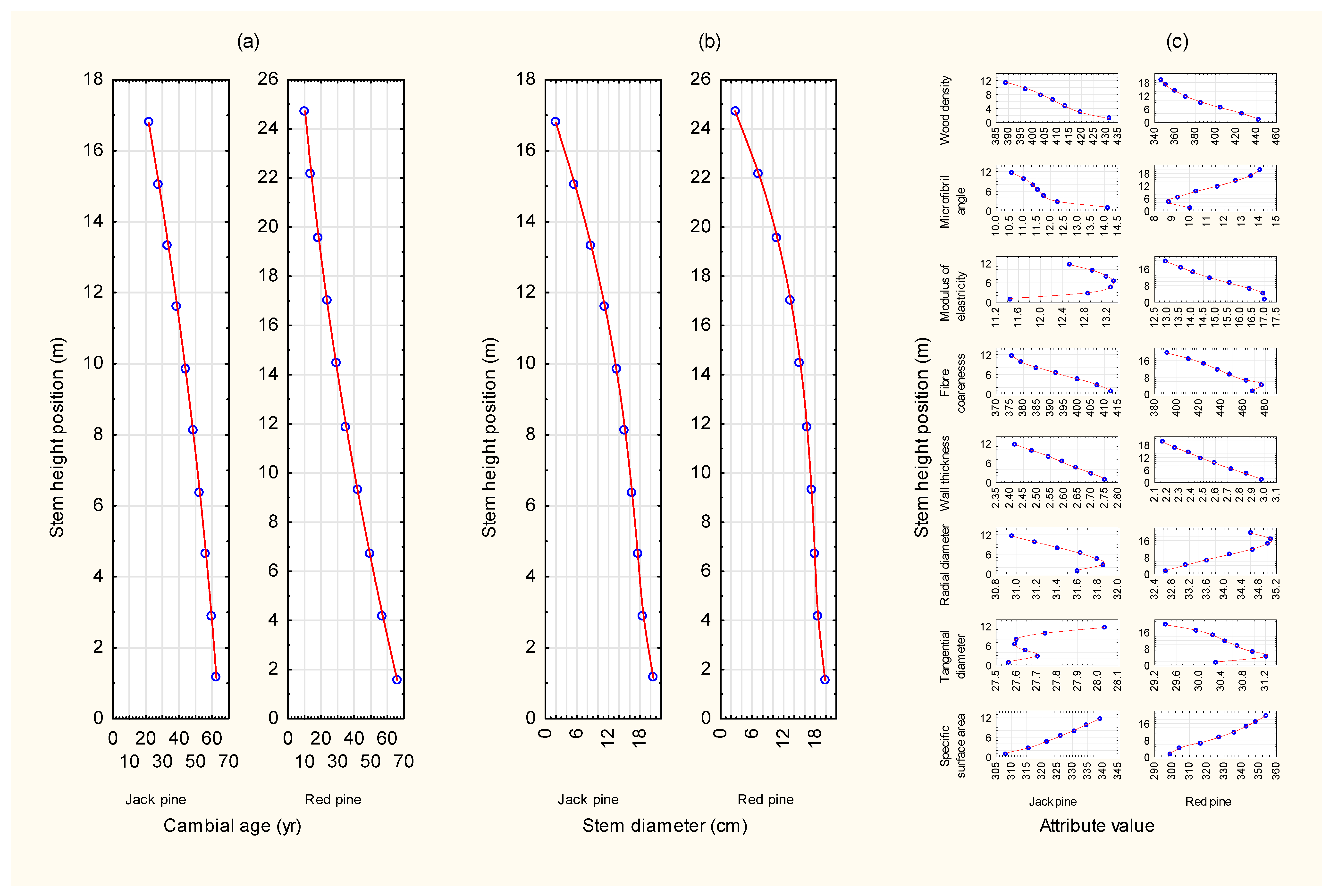
Secondly, the species-specific attribute equation suites along with the respective cambial age–stem height equations were then incorporated into the jack pine and red pine SSDMMs via the Silviscan-based Fibre Attributes Module, as schematically illustrated in Figure 1 of [6]. The resultant SSDMM algorithms enabled the generation of attribute estimates throughout the entire stem for trees within each recovered diameter class. More precisely, for a specified crop plan, the predicted size–density trajectory and recovered grouped diameter distribution were used to generate attribute estimates for each diameter class across all specified stem height positions, deploying the embedded models. Figure 3 graphically exemplifies these species-specific predictions along with the upper cambial age and stem diameter estimates for the mean-sized tree (quadratic mean diameter) at rotation for the control crop plans (Regime 1 as specified in Table 1). As illustrated in Figure 3, the incorporated cambial age–stem height position equations (Equation (3); Table 2) yielded the prerequisite upper stem cambial age estimates (Figure 3a) and the embedded taper equations generated the prerequisite upper stem diameter estimates (Figure 3b). These predictions along with breast-height diameter, total tree age, and total height estimates, which were calculated internally within the SSDMMs, were then used to populate the species-specific whole-stem fibre attribute equations. Thus enabling the prediction of eight end-product fibre attribute determinates throughout the entire tree stem, e.g., at 5, 15, …, 95 percentile-based height intervals, as shown in Figure 3c for a rotational mean-sized tree. A complete tabular exemplification of all the rotational predictions inclusive of stem-based dimensional metrics and values for all eight attributes by stem height position for each species is provided in Table 3 for the tree of mean quadratic diameter produced by each regime.

3.2. Crop Planning Exemplifications

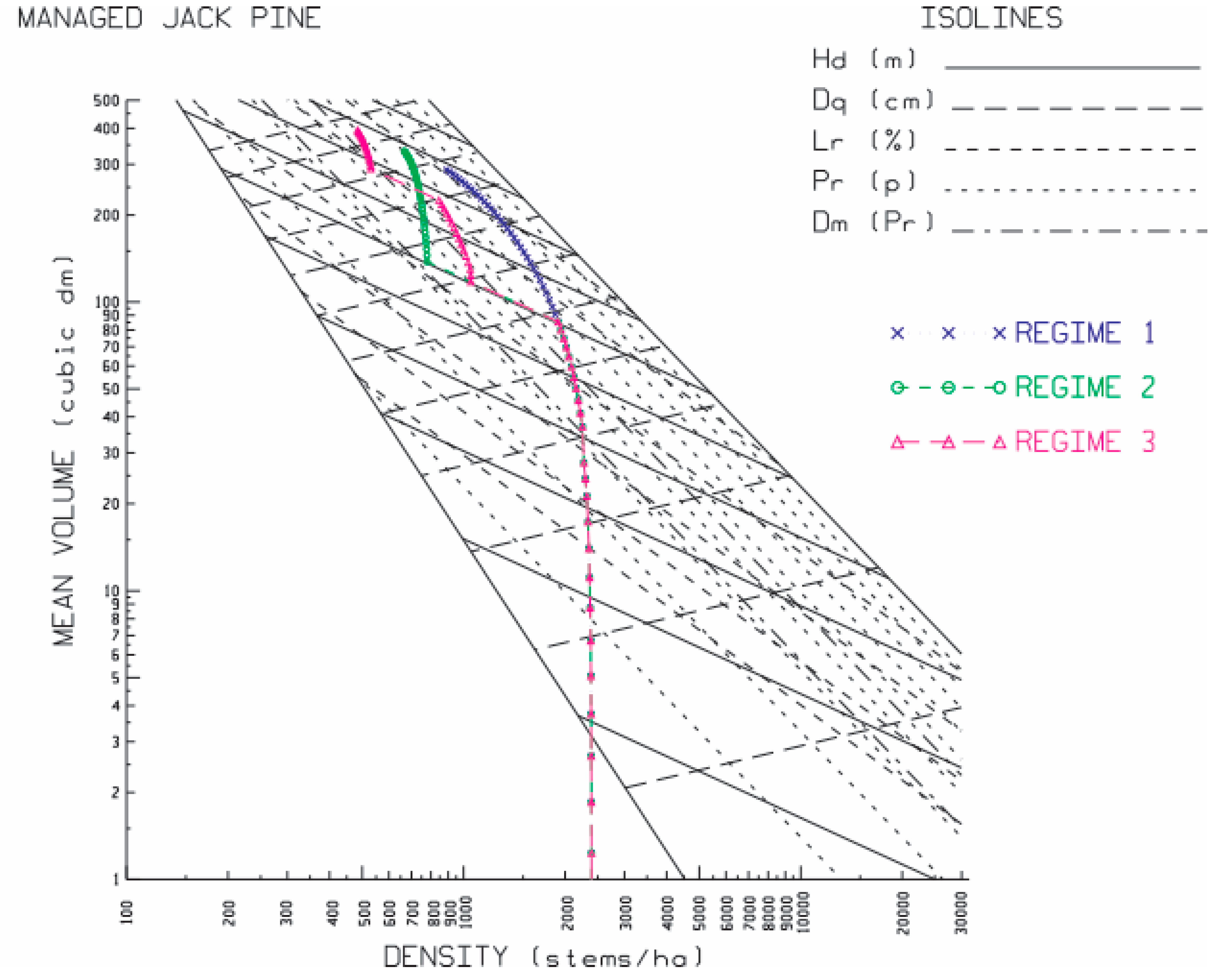
The resultant species-specific temporal size–density trajectories for the locale-specific crop plans growing under conditions consistent with a RCP4.5 climate change scenario on medium-to-good site qualities are illustrated within the context of the traditional stand density management diagram, in Figure 4 for jack pine and in Figure 5 for red pine. As inferred from the jack pine graphic, the plantations attained crown closure status by age 10 as determined from the site-based age equivalent of the mean dominant height value where the size–density trajectories and crown closure line intersect (i.e., 4 m, which, on this site index, is attained at approximately 10 yr). Self-thinning subsequently commenced and continued until rotation age with losses within the merchantable size classes initiating by age 30. The dominant height, mean quadratic diameter, density, stocking, relative density, and mean live crown ratio of the plantation at the time of the first CT treatment (30 yr; Regimes 2 and 3) were 14 m, 11 cm, 1906 stems/ha, 28 m2/ha, 0.56, and 43%, respectively. At the time of the second CT treatment (45 yr; Regime 3), these values were 17.5 m, 20 cm, 845 stems/ha, 26 m2/ha, 0.56, and 39%, respectively. Although the plantations at the time of the thinning treatments were above their optimal site occupancy levels (0.32 ≤ relative density ≤ 0.45) and incurring density-dependent mortality losses within the merchantable size classes, structurally they met the provincial-based regulatory guidelines for CT (e.g., minimum pretreatment basal area of 25 m2/ha and a live crown ratio of 35%; OMNRF [33]). Total and merchantable density mortality losses during the post-thinning period (31–65 yr) were much greater in the unthinned plantation: i.e., total density losses of 1015 stems/ha for Regime 1 versus 117 stems/ha for Regime 2 and 245 stems/ha for Regime 3. The thinning regimes avoided approximately 86% (Regime 2) and 71% (Regime 3) of the expected merchantable density losses when compared to the unthinned plantation over the 31–65 year rotational period (i.e., 783 abiotic stems/ha for Regime 1 versus 106 abiotic stems/ha for Regime 2 and 228 abiotic stems/ha for Regime 3). The thinning regimes also yielded larger mean-sized trees and a greater number of merchantable-sized trees over the rotation: (1) 21 cm (Regime 1) versus 23 cm (Regime 2) and 25 cm (Regime 3) in quadratic mean diameter; and (2) 891 stems/ha (Regime 1) versus 1568 stems/ha (76% increase; Regime 2) and 1416 stems/ha (59% increase; Regime 3).
Similarly, as inferred from the red pine diagram (Figure 5), the forecasted size–density trajectories attained crown closure status by age 12. Again, this was determined from the site-based age equivalent of the mean dominant height value corresponding to the intersection of the size–density trajectories and the crown closure line (i.e., 6 m, which, on this site index, is attained at approximately 12 yr). Self-thinning within the merchantable size classes was initiated at age 25. The dominant height, mean quadratic diameter, density, stocking, relative density, and mean live crown ratio of the plantations at the time of the first CT treatment (40 yr; Regimes 2 and 3), as extracted from the size–density trajectory and the 20 m dominant height isoline intersection point, were, respectively, 20 m, 17 cm, 1850 stems/ha, 42 m2/ha, 0.38, and 36%. At the time of the second CT treatment (55 yr; Regime 3) these values were, respectively, 24 m, 23 cm, 1019 stems/ha, 44 m2/ha, 0.39, and 39%. Although the plantations at the time of the thinning treatments were within the optimal site occupancy window (0.32 ≤ relative density ≤ 0.45), they were incurring density-dependent mortality losses within the merchantable size classes. Like the jack pine plantations, the red pine plantations were in compliance with the provincial-based regulatory guidelines for CT (OMNRF [33]). Total and merchantable density mortality losses during the post-thinning period (41–70 yr) were greater in the unthinned plantation: 280 stems/ha versus 117 stems/ha in Regime 2 and 120 stems/ha in Regime 3 (note, all stems were of merchantable size). Hence, the thinning regimes captured approximately 58% of the expected merchantable density loss when compared to the unthinned regime. Although the thinning regimes only produced 10% more merchantable-sized stems by rotation (i.e., 1570 stems/ha for Regime 1 versus 1716 stems/ha for Regime 2 and 1725 stems/ha for Regime 3), they were much larger in size (i.e., 23 cm (Regime 1) versus 29 cm (Regime 2) and 31 cm (Regime 3) in quadratic mean diameter) with the twice-thinned regime actually yielding pole size material by rotation.
A summary of the species-specific rotational yield outcomes and management performance indicators for each crop plan set is provided in Table 4. These rotational measures along with the volumetric loss metrics arising from the underlying density-dependent and density-independent mortality processes were included as secondary but important criteria when evaluating the crop plans. The generation of standing and fallen deadwood can be positive for biodiversity maintenance and in some jurisdictions suggested volumetric thresholds have been proposed (e.g., [34]). Conversely, the production of excessive amounts of abiotic masses can be detrimental to carbon balances (e.g., increasing decay-based carbon emissions) and wildfire risk mitigation (e.g., increased laddering potential from the presence and vertical distribution of standing abiotic trees and bridge fuels (sensu [35])). Thus, based on the varied European biodiversity-based thresholds recommended for northern forests, this study accepted that the deployment of a 30 m3/ha rotational-long threshold would be a reasonable deadwood accumulation target for either species.
The results, as presented in Table 4 for the conventional rotational yield and performance metrics, indicated that thinning as expected increased mean tree size for both species with the twice-thinned regimes exhibiting the greatest improvements (i.e., respectively, 8% and 18% for jack pine Regimes 2 and 3, and 28% and 36% for red pine Regimes 2 and 3). Stocking levels fell within the thinned plantations by 13% and 27% for jack pine Regimes 2 and 3, respectively, and by 30% and 36% for red pine Regimes 2 and 3, respectively. Merchantable and total volumetric productivity increased within the thinned jack pine plantations (e.g., increases in merchantable volume over the rotation of 7% and 4% for Regimes 2 and 3, respectively, relative to Regime 1). However, such volumetric productivity declined within the thinned red pine plantations (e.g., declines of 15% and 13% for Regimes 2 and 3, respectively, relative to Regime 1). The production of deadwood declined with increasing thinning frequency irrespective of species (e.g., decreases of 73% and 61% for jack pine Regimes 2 and 3, and 24% for red pine for both regimes). Stand stability improved with thinning, as evident from the reduction in the height–diameter ratio (<100) for both species. Economically, the once-thinned jack pine plantation and both of the thinned red pine plantations yielded positive relative increases in land expectation values when compared to their unthinned counterparts (Regime 1). The once-thinned jack pine plantation (Regime 2) and the twice-thinned red pine plantation (Regime 3) were selected as the optimal regimes for these specific of crop plan sets, i.e., over the rotation, these regimes delivered larger mean tree sizes, increased volumetric production (jack pine only), produced greater proportions of commercial-useable wood fibre, provided sufficient abiotic coarse woody debris for biodiversity maintenance, yielded stable stand structures, and enhanced overall economic worth.
The results, as presented in Table 5, in terms of the quality and quantity of HWPs produced by each jack pine regime, indicated that the rotational volumetric percentage of SW HWPs marginally increased for the thinned plantations and that such HWPs were extractable at each thinning entry, irrespective of regime. However, the twice-thinned plantation yielded a dramatic increase in the production of extractable SW HWPs during the second entry (e.g., from 5 to 58%). Conversely, the NSW HWPs dominated the product yields during the first entry (e.g., 92% and 95% for Regimes 2 and 3, respectively). Age equivalent comparisons of the mean wood attribute values by product type (SW and NSW HWPs) did not consequentially differ across the regimes. Likewise, no grade-based differentiation was observed (i.e., all SW HWPs produced were classified as belonging to the low quality class). Notably, wood density was the attribute responsible for the downgrade, e.g., all SW HWPs exceeded the minimum Me threshold for the medium quality class (12.1 GPa); however, wood density values were considerably lower than the minimum Wd threshold (441 kg/m3).
The corresponding results, as presented for red pine in Table 6, indicated that the rotational volumetric percentage of SW HWPs also increased for the thinned plantations, although their grade quality class was rated as low. Furthermore, the thinning treatments did not produce any SW HWPs irrespective of regime. Only the regime with two thinning treatments was able to produce high value pole-sized trees by rotation. Contrary to the jack pine results, rotational comparisons of the mean wood attribute values by product type (SW and NSW HWPs) did differ between the unthinned and thinned plantations. Essentially, the quality of the SW HWPs with respect to extractable dimensional lumber products produced by the thinned plantations was lower than that of the unthinned plantation. This was mostly due to the higher Ma and lower Me values. Conversely, attributes underlying the EPP of NSW HWPs with respect to pulp and paper products increased with thinning frequency, e.g., higher Co and lower Sa values. Similarly to jack pine, lower wood density values negated the movement of the extractable SW HWPs into the higher quality classes, irrespective of regime. In fact, the minimum Me threshold for the highest quality class was exceeded while the wood density values did not even attain the minimum Wd threshold required for the medium quality class.
Considering both the conventional yield metrics and HWP production in terms of both quality and quantity for these species-specific crop planning exemplifications indicates the following optimal regime selections. For jack pine, the once-thinned plantation (Regime 2) was selected given that it would deliver increases in volumetric yield, reductions in abiotic mass generation, and positive economic returns without consequentially affecting the proportion or quality of the HWPs produced. For red pine, the twice-thinned plantation (Regime 3) was selected given that it would yield increases in mean tree size, reductions in abiotic mass production, increases in economic worth, increases in stand stability, and attainment of pole production status, all while not consequentially affecting the proportion or quality of the HWPs produced. Notably, the inference that wood density was the limiting attribute-based determinate responsible for the lower grade classifications for the SW HWPs for both species suggests that the wood quality of thinned plantations may be inferior to comparable unthinned plantations. Most plausibly due to the increased annual ring increment (growth) that accompanies thinning treatments that could lead to lower density wood at rotation (e.g., as evident from the increased mean tree sizes presented in Table 4 for the thinned plantations).

3.3. Whole-Stem Attribute Developmental Maps

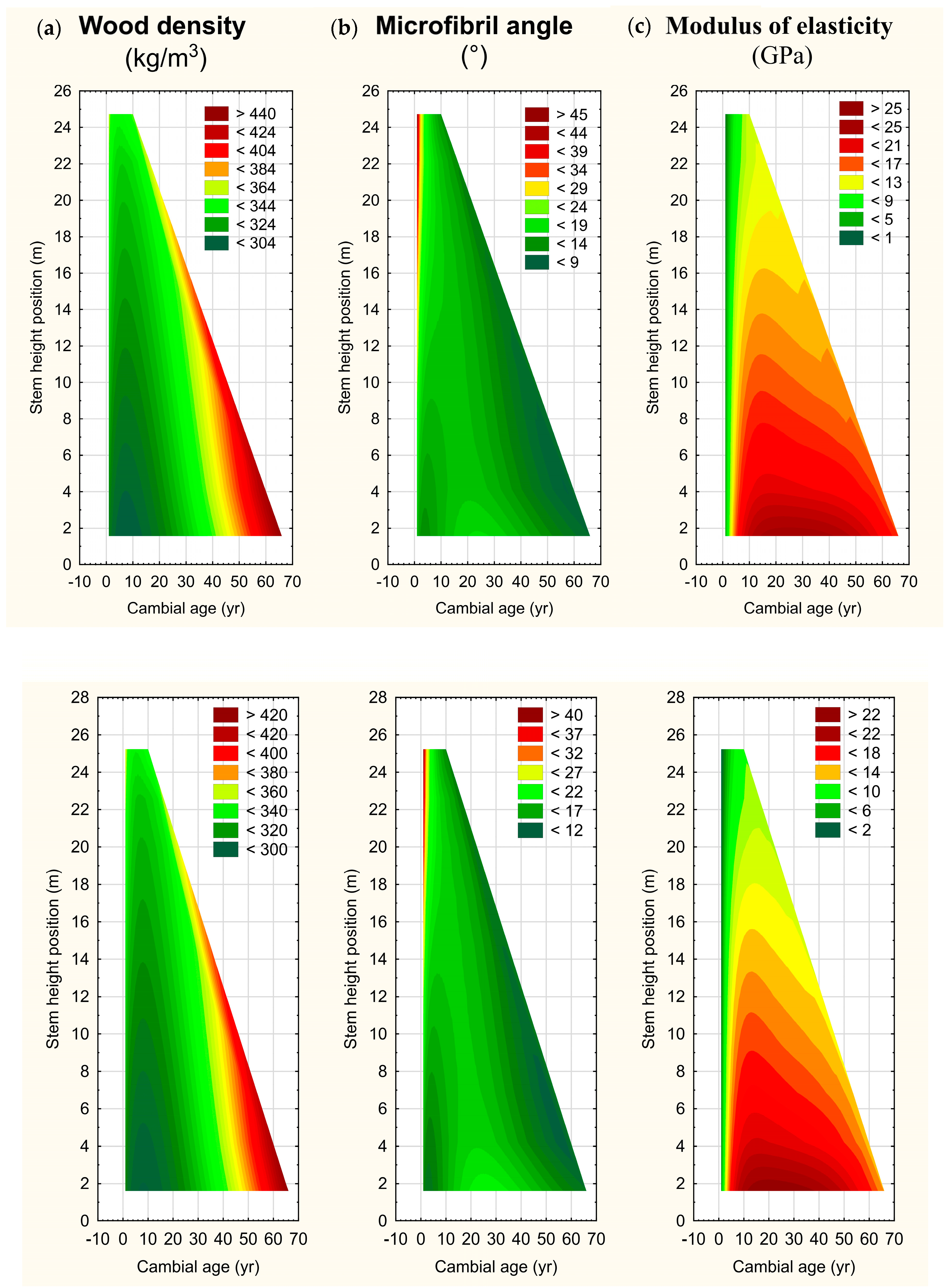
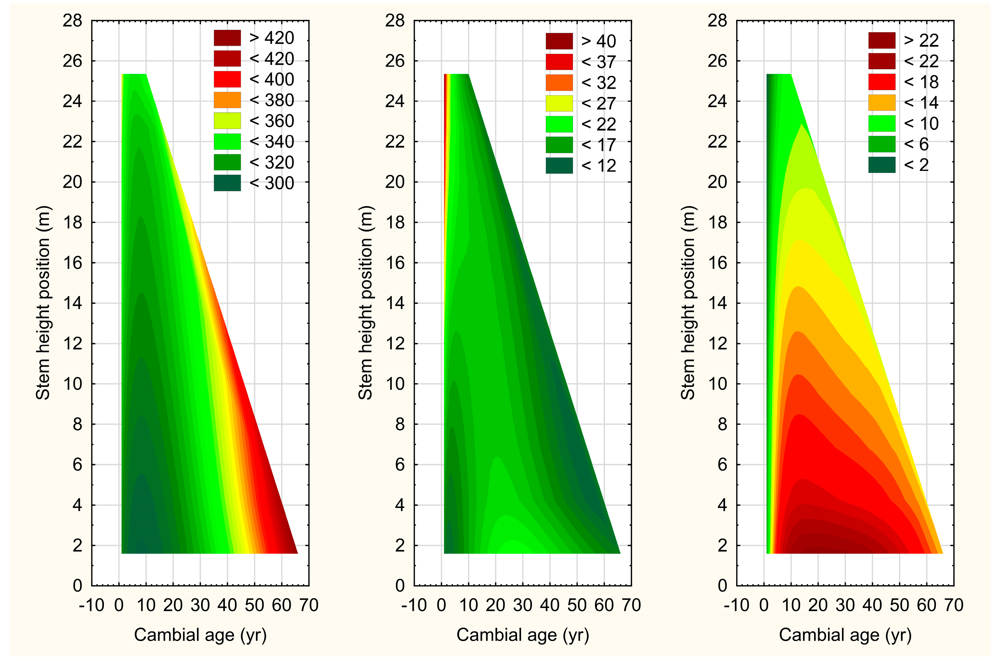
Computationally, deploying the species-specific (1) previously developed attribute prediction equations (Equation (5) and Table 4 in [7]), (2) cambial age prediction equations (Equation (3) and Table 2), (3) previously developed height–diameter functions ([30] for jack pine and [6] for red pine), and (4) previously developed taper equations ([31] for jack pine and [32] for red pine), the enhanced SSDMMs were also used to produce a set of annual-based cumulative attribute values for three of the key end-product determinates (Wd, Ma, and Me). Specifically, by generating estimates for each attribute at the 5, 15, …, 95 percentile-based height positions for the tree of mean quadratic diameter for each regime. These annual estimates were then used to construct triangle-based data-centric 3-dimensional surfaces using a wafer-based graphical algorithm, which ultimately yielded whole-tree attribute maps. In order to provide an inferential framework when interpreting the cumulative attribute maps, the resultant Me wafer plot for the mean-sized tree (mean quadratic diameter = 22 cm) at rotation (65 yr) for the jack pine crop plan denoted Regime 1 (Figure 4; Table 1) is first presented in Figure 6. This figure illustrates the cumulative value for Me throughout the vertical and horizontal profile of the main stem of the mean-sized tree (i.e., at the 5 to 95 height percentiles by cambial age). The predicted 52 and 65 year-old values are contrasted for the 10 m stem height position. The resultant Me values of 11.4 and 13.0 reflect the overall wood stiffness of the entire cross-sectional disc at the 10 m stem height position at age 52 and 65, respectively, thus reflecting the evolution of the solid wood potential at this stem position. The solid wood potential at this stem height if harvested at age 52 and 65 suggests that harvesting at either date would potentially yield extractable SW HWPs (i.e., dynamic Me predictions exceeded the static-based Me threshold of 8.2 required for dimensional lumber status (sensu NLGA [20])). However, this would also be conditional on attaining the corresponding Wd minimum threshold value required for dimensional lumber. Additionally, knowing total tree age, number of years required to reach a specific tree height, and cambial age, the maps can be used to infer the age at which a tree is able to produce HWPs and their associated grades. For example, the map presented in Figure 6 suggests that the Me threshold for SW HWPs (Me > 8.2 GPa) would be attained within the lower stem region (≤6 m) at approximately 35 years post-establishment. This can be determined as follows: (1) calculating the number of years required to reach a height of 6 m (i.e., total tree age (65) − total age of the cross-sectional disc (52) yields 13 years); (2) adding the cambial age at which a minimum 8.3 GPa is attained at the 6 m stem height position (i.e., 22 years); and (3) given (1) and (2), yields 13 + 22 = 35 years, the age at SW HWPs are potentially produced. Although Figure 6 provides guidance for interpreting the subsequent maps presented in Figure 7 and Figure 8, it is informative to acknowledge two overriding beneficial characteristics of the cumulative moving average metric. Firstly, it is a composite descriptive statistic that accounts for all preceding values of a temporally ordered annual ring attribute sequence (Equation (1)). Hence, area-based weighting of these preceding annual ring values and carrying forward their cumulative effect act to computationally dampen the effect of environmentally induced annual fluctuations. Secondly, it can be more reflective of long-term attribute development trends than other measures of central tendency (e.g., arithmetic mean) and hence may have more inferential utility in terms of assessing the temporal evolution of EPP than other average-based descriptive statistics.
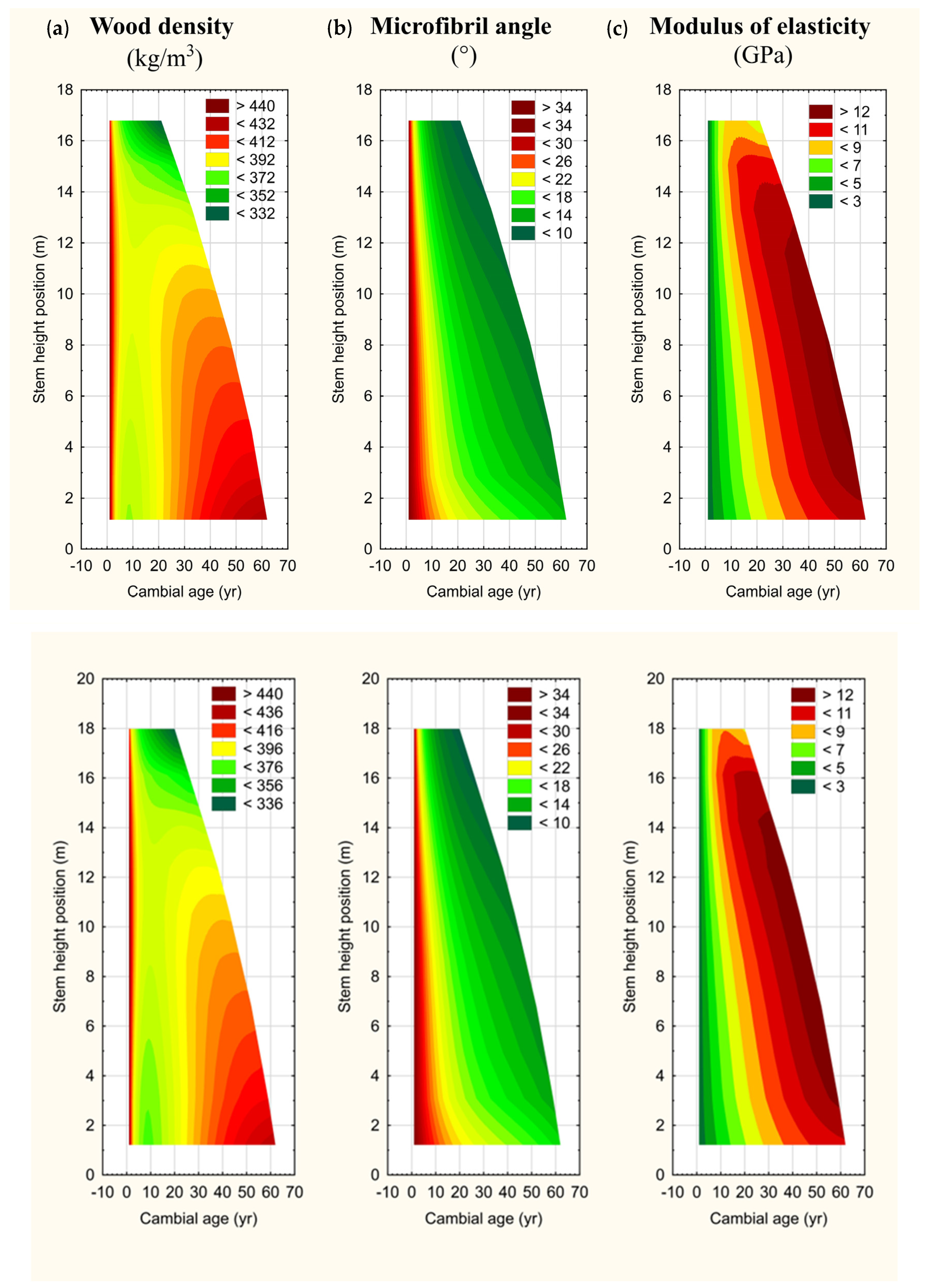
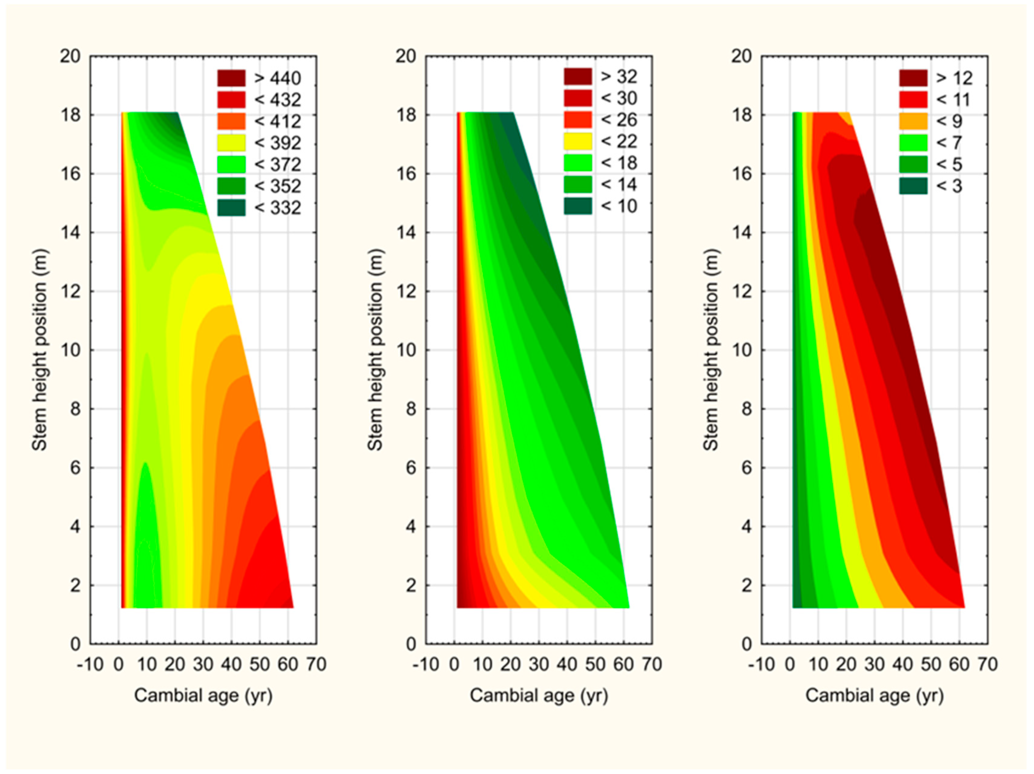
Figure 7 and Figure 8 provide the rotation-long exemplifications of the Wd, Ma, and Me cumulative developmental maps for the tree of mean size for each crop plan by species. Deployment of the standardized grading specifications as surrogate performance indicators for inferring EPP provides a more explicit inference with respect to potential product grade assortments for a given crop plan. For example, examining the wood property maps for wood density and the modulus of elasticity for the mean-sized tree generated at rotation from three jack pine regimes along with the corresponding maps for Ma (Figure 7) reveals that wood fibre extracted from the lower-to-middle stem regions (0.1 to 0.5 relative height) would potentially produce low to medium quality dimensional lumber products (NLGA [20]): e.g., Wd > 400 (kg/m3) (outer reddish region) and Me >> 8.3 GPa (outer greenish and reddish regions) while not being downgraded or rejected due to intolerable Ma values (e.g., Ma < 20°; outer greenish region). Conversely, wood fibre extracted from the middle-to-upper stem regions (>0.5 relative height) would potentially only produce NSW HWPs given the problematic wood density values (Wd < 400 (kg/m3); outer yellowish to greenish regions). Although these interpretations for the mean-sized trees (22, 24, and 26 cm diameter) were consistent across the regimes, whole-stem SW HWP potential did marginally increase with increasing tree size with respect to Wd but not to Ma or Me. Slight differences in the vertical distribution patterns with increasing size was evident across all the regimes, i.e., Wd   Dq, Ma   Dq−1, and Me   Dq−1, for all merchantable stem height positions (note, Dq denotes quadratic mean diameter). However, these marginal attribute differences would not likely elicit grade-based changes in the quality of SW HWPs potentially extractable.
Likewise for red pine, examining the Wd, Ma, and Me wood property maps for the mean-sized tree generated at rotation across regimes (Figure 8) revealed that wood fibre extracted from the lower third of the stem (0.1 to 0.3 relative height) would potentially produce low quality dimensional lumber products (NLGA [20]): e.g., Wd > 400 (kg/m3; outer light to dark red regions), Ma < 20° (outer light to dark green regions), and Me >> 8.3 GPa (outer light to dark green regions). Conversely, wood fibre extracted from the middle and upper stem regions (>0.3 relative height) would potentially only produce NSW HWPs given the problematic wood density values (Wd < 400 (kg/m3); outer yellowish to greenish regions). Although these interpretations for the mean-sized red pine trees (22, 28, and 30 diameter-sized trees) were generally consistent across the regimes, whole-stem SW HWP potential did decline with increasing tree size, i.e., Wd and Me   Dq−1 for any given merchantable stem height position.

4. Discussion

4.1. End-Product Potential (EPP) of HWPs: Concepts, Correlates, and Forecasting

Functionally, the EPP of HWPs extracted from an individual jack pine or red pine tree stem or harvested log is largely a function of its external morphological and internal anatomical characteristics. Physical size, geometric form, and size and frequency of residual surface knots are among the most important external determinates of the EPP of HWPs [36,37]. For example, the EPP of a harvested tree stem or extracted log is directly proportional to its diameter, length, and straightness, and inversely proportional to its taper and knottiness. Among the most important internal xylem-based determinates underlying the EPP of HWPs are Wd, Ma, Me, Co, Wt, Dr, Dt, and Sa (sensu [38]). For example, the EPP of long-lived SW HWPs such as dimensional lumber, square timbers, and utility poles is directly proportional to Wd (strength) and Me (stiffness) and inversely proportional to Ma (strength and stiffness). The EPP of short-lived NSW HWPs such as pulp and paper products (e.g., paperboards, newsprint, and facial tissues) is directly proportional to Wd (yield), Wt (tensile strength), Dr (bulk), Dt (bulk), Sa (tensile strength), and Ma (stretch) and inversely proportional to Co (tensile strength). The EPP of very short-lived NSW HWPs such as fossil fuel-displacing wood pellets used for thermal energy generation is directly proportional to Wd (heating value). Although external and internal correlates are of consequential utility when attempting to estimate EPP of HWPs, the latter correlates provide a more definitive account of EPP given their explicit relationship with individual performance measures that are used to classify and grade extractable end-products (sensu [20,38]). Logistically, a number of these key internal EPP attribute-based determinates for standing trees and harvested logs can be readily determined via non-destructive or destructive sampling-based approaches [39]. For example, innovative non-destructive sampling tools such as acoustic velocity instruments and microdrills were developed to estimate a number of these internal end-product-based attribute-determinates (e.g., dynamic modulus of elasticity and wood density, respectively [40,41,42,43]). Likewise, increment core sampling of standing trees or destructive cross-sectional sampling of harvested logs followed by Silviscan analysis can yield a suite of wood attribute estimates that can be quite informative when attempting to infer EPP.
Although the utility of these indirect and direct approaches to attribute determination in pre-harvest and post-harvest EPP assessments has been well established (sensu [41,43]), the ability to forecast the EPP of HWPs within the context of crop planning and silvicultural decision-making has not yet reached a similar level of maturity [44]. Explicitly predicting end-product outcomes arising from stand-level management interventions, such as initial spacing control and precommercial and commercial thinning treatments, is inherently challenging in Canada given the paucity availability of such enabled crop planning decision-support tools (sensu [2]). Historically, this deficiency has partially arisen from the modelling choices that have justifiably been focused on volumetric yield estimation given its importance in regulated forest management planning (e.g., development of empirical bench-mark yield curves required for generating annual allowable cut levels [45]). However, even if individual tree wood quality prediction models were available, most of the currently available volumetric-based forecasting models are analytically incapable of incorporating such and predicting resultant end-product outcomes. Principally, due to their inability to generate the horizontal (diameter) and vertical (height) size distributions that are essential prerequisites for deriving EPP estimates of HWPs at the individual tree, diameter class, and stand levels. Hence the ability to design optimal silvicultural-based crop plans with respect to maximizing the production of long-lived HWPs remains a challenging endeavour.
Fortunately, SSDMMs provide the analytical foundation for estimating commercially relevant wood quality attributes across a stand’s size distribution when augmented by spatially invariant fibre attribute prediction equations [5,6]. Furthermore, embedding SSDMMs with spatiotemporal whole-stem equations should yield enhanced crop planning tools that are capable of providing a more complete EPP account of extractable HWPs. Thereby increasing the resolution and precision of climate-sensitive crop plan forecasts with respect to the quantity and quality of end-products produced and, by extension, the potential carbon storage and substitution value of HWPs, as shown and exemplified in this study. Specifically, the development and integration of the tertiary-level hierarchical mixed-effects attribute equation suites and the two-level hierarchical mixed-effects upper-stem cambial age prediction models within the SSDMMs provided the inferential framework for evaluating the EPP of all extractable HWPs when crop planning. A critical step underlying the realization of the enhanced SSDMMs was the development of the unbiased, well fitting, and relatively precise whole-stem cambial age prediction models (e.g., index of fits (proportion of dependent variable variation explained) and SEEs (yr), respectively, of 0.995 and 1.1 yr for jack pine and 0.996 and 1.4 for red pine). The resultant SSDMMs with their embedded spatiotemporal attribute equation suites yielded improvements in the precision and resolution of EPP predictions relative to the previous generation of crop planning tools. Particularly when considering that such tools only incorporated spatially invariant attribute equation suites and thus could only provide EPP estimates at a single stem position (breast-height; [5,6]). Operationally, this enhanced predictive ability enriches and improves end-product forecasting with respect to estimating the quality and quantity of HWPs along with their carbon storage and substitution potentials when crop planning.
As exemplified in this study, examination of the species-specific attribute prediction trends throughout the entire vertical stem profile across all size classes provided a framework to extract attribute developmental patterns and generalized inferences regarding end-product potentials (e.g., Figure 7 and Figure 8 and Table 5 and Table 6). Furthermore, with respect to the predictive performance of the enhanced SSDMMs in terms of inferring EPP from predicted fibre attribute values, the tabular estimates and graphical-based predicted trends for all eight attributes were in general concordance with those observed within the underlying Silviscan-derived attribute data sets used for model parameterization. For example, numerically comparing the predicted attribute trends with those within the sample attribute data sets (Table S2a (jack pine) and Table S2b (red pine) in [7]) suggested general agreement. Exceptions to this inference were only evident for jack pine in which fibre coarseness and tracheid tangential diameter attribute predictions within the upper stem regions exhibited divergent nonlinear trends as the stem apex was approached.
Given that the rotational attribute predictions and extracted end-product inferences are unique to the specified crop plan sets, caution should be exercised when inferring generalized trends of these species to density management treatments. Furthermore, the lack of explicit linkages between Silviscan-derived attribute estimates and end-product-specific attribute-based performance metrics (e.g., grade-based Wd and Me ranges for SW HWPs), the EPP inferences should also be considered as informed approximations. Notwithstanding these limitations, conditional inferences can nevertheless be drawn given the association between attributes and end-product performance measures (sensu [38,46]). Sorting and fine scale estimation of the EPP of SW and NSW HWPs are achievable by employing grade-based attribute ranges for the various HWP types. Principally, because these attribute determinates which underlie the type (e.g., SW versus NSW based on Wd and Me minimum thresholds) and quality of SW HWPs (e.g., low, medium, and high grade based on Wd and Me thresholds ranges) have been well defined in various grading systems (e.g., [20]).
Scaling and deploying these associations and threshold ranges when examining whole-stem diameter class-specific attribute profiles generated for a given crop plan enables a determination of the plausibility of attaining stand-level HWP production objectives. To demonstrate such, rotational whole-stem end-point profiles are presented in the Supplementary Material, i.e., rotational whole-stem end-point profiles for Wd, Ma, Me, Co, Wt, Dr, Dt, and Sa are presented by diameter class for each (1) jack pine crop plan in Figures S1a, S1b, S1c, S1d, S1e, S1f, S1g, and S1h for, respectively, and (2) red pine crop plan in Figures S2a, S2b, S2c, S2d, S2e, S2f, S2g, and S2h, respectively. Briefly examining these profiles in terms of stem height and size dependent patterns with respect to the EPP of SW and NSW HWPs yielded the following inferences. For jack pine, the whole-stem EPP of SW HWPs increased with increasing tree size (i.e., Wd and Me  Dc (diameter class)) with the largest gains attributed to the concurrent increased height invariance in Me (i.e., Me did not decline consequentially with increasing stem height position (Hr)). The EPP of NSW HWPs increased with tree size and with stem height particularly within the upper stem region (Co   Dc1 for Hr > 50%; Wt   Dc; Dr   Dc; Sa  Hr) and conversely declined with increasing tree size within the lower stem regions (Sa   Dc1 for Hr < 50%). For red pine, the EPP of SW HWPs marginally declined with increasing tree size (Ma   Dc becoming more consequential in the mid-upper stem region). The EPP of NSW HWPs was largely invariant to tree size although the predicted height-based increases in Sa could result in improved EPP with respect to pulp and paper products. It is evident from these exemplifications that the whole-stem EPP of SW and NSW HWPs will vary by tree size and stem region. In order to attain a stand-level perspective on whole-stem EPP, individual tree inferences must be scaled to the stand-level according to the underlying size-based volume frequency distribution, particularly given that thinning treatments generally shift the evolution of the size and volume distribution towards the larger size classes. The HWP volume metrics and associated grade estimates that are presented in Table 5 and Table 6 are such scaled estimates.
In summary, the deployment of the attribute equation suites within the SSDMMs and their subsequent exemplification in crop planning decision-making demonstrated the importance of accounting for whole-stem attribute variation when forecasting the EPP of HWPs. Operationally, however, limitations to the accuracy of the HWP forecasts produced by the presented crop planning models may exist given the restricted range of the parameterization data sets deployed. For example, the jack pine attribute data were extracted from sample trees that had initially regenerated naturally following wildfire and developed under a range of density–stress levels (e.g., unthinned to thinned stand conditions). Consequently, when such calibrated equations are integrated into SSDMMs, cumulative rotational estimates for variates such as microfibril angle and modules of elasticity may be underestimated and overestimated, respectively, for plantation simulations. Although the red pine attribute data sets were extracted from plantations, they were intensely managed in terms of density management treatments (e.g., sequentially thinned multiple times over their rotations (n > 3)). However, contrary to the jack pine situation, the rapid growth response following each thinning could result in the overestimation of variates such as microfibril angle and the underestimation of the modules of elasticity. Hence, caution should be exercised when explicitly interpreting the rotational attribute values and associated end-product inferences generated from simulations.

4.2. Tree-Level Fibre Attribute Mapping and Individual Tree HWP Inferences

Innovative advancements in attribute determination methods inclusive of X-ray densitometry, Silviscan, and near-infrared spectroscopy have set the stage for advanced within-stem attribute mapping (e.g., descriptive graphical interpolation methods [47,48,49,50,51]) and model development (e.g., empirical prediction modelling [52,53]). In reference to the graphical approaches, Defo [47] developed a triangular-based whole-stem mapping algorithm for graphically presenting Silviscan-derived individual annual ring attribute estimates for destructively sampled trees (EvaluTreeMap). They demonstrated the utility of the approach by contrasting the fibre coarseness profiles and associated descriptive statistical metrics between diseased (Armillaria ostoyae) and disease-free interior Douglas fir (Pseudotsuga menziesii (Mirb.) var. glauca (Bessin.) Franco) trees. Schimleck [48] deployed an Akima-based interpolation approach to formulate whole-stem property maps for wood density, microfibril angle, and modulus of elasticity within loblolly pine (Pinus taeda L.) trees. They subsequently investigated the effect of plantation age on these distributions within the context of end-product potential. Additional property maps and associated inferences were similarly presented by Schimleck [54] for other commercially relevant fibre attributes (e.g., fibre coarseness, tracheid wall thickness, radial and tangential diameters, and specific surface area).
Duff and Nolan [55,56] provided an analytical-based inferential framework for interpreting the spatiotemporal whole-stem development patterns of excurrent coniferous tree species. Briefly, horizontal sequences were denoted as pith-to-cambium radial developmental patterns at specific stem height positions whereas oblique sequences were denoted as age-specific stump-to-apex vertical developmental patterns. The fibre attribute models in combination with the cambial age prediction models as deployed within the SSDMM framework enabled the generation of 3-dimensional graphical representations of whole-stem attribute profiles from which Duff and Nolan like inferences could be extracted. For example, extracting retrospective whole-stem cumulative attribute developmental patterns. These patterns facilitated the estimation of age-specific cumulative developmental states from which end-product potentials could be inferred (e.g., Figure 7 and Figure 8). Specifically, for jack pine, the radial developmental patterns in wood density followed a consistent pattern irrespective of height position, suggesting an invariant horizontal dependency (Figure 7): values initially increased and then briefly declined before resuming an increasing trend with increasing cambial age irrespective of stem height position. The oblique sequence for wood density indicated a height-dependent stump-to-apex decline (Figure 7): wood density declined with increasing stem height position for a given development state (cambial age). Examining the patterns for microfibril angle (Figure 7) revealed rapid pith-bark radial declines irrespective of the stem height position. These horizontal trends are consistent with expectation in that the higher values near the pith are reflective of the formation of juvenile wood arising from localized crown formation or open-grown conditions before the commencement of crown closure status (sensu [57]). The oblique sequence indicated relatively stable increasing trends: values for any given cambial age increased with increasing stem height position. The horizontal pattern for the wood stiffness metric, the modulus of elasticity as shown in Figure 7, revealed increasing linear-like trends with increasing cambial age across all height positions. The oblique sequence indicated slightly increasing height-dependent trends where elasticity values for any given cambial age increased with increasing stem height position until the very upper stem region was reached. Essentially these trends imply that lumber-producing potential within these exemplified mature sawlog-sized jack pine trees increased temporally with increasing age and spatially with declining stem height (e.g., density and elasticity values maximizing within the lower stem regions).
Likewise, for the exemplified mature sawlog-sized red pine trees, the retrospective cumulative developmental trajectories for wood density (Figure 8) exhibited a nonlinear-like horizontal pattern where values exhibit a gradual then rapid temporal increase particularly within the lower bole region. Conversely, a relatively constant oblique trend was evident in which values for any given age remained relatively constant with increasing stem height. Although the microfibril angle was relatively age invariant irrespective of height position, the values did minimize during the period following juvenile wood formation (≈20 yrs; Figure 8). The temporal horizontal and height-dependent oblique trends observed for the modulus of elasticity contrasted to that observed for jack pine (c.f., Figure 7 versus Figure 8). Specifically, in red pine, radial values maximized within the lowest stem regions and temporally before maturity was reached (i.e., unique lower-bole (<12 m) increasing concentration of high wood stiffness values with decreasing height across a wide developmental range (5–65 yr cambial age range)). Collectively, these trends suggest that lumber-producing potential within these mature sawlog-sized red pine trees was maximized within the lower central region of the stem.
Although acknowledging that the dynamic-based Me estimates obtained via Silviscan commonly overestimate its static-based counterpart (e.g., +25% in loblolly pine (Pinus taeda L.); [58]) and that design-based specifications for machine stress-rated (MSR) dimensional lumber deploy the latter [20], extracting conditional inferences regarding end-product potential can nevertheless be informative (e.g., [5]). For example, the MSR-based mean specifications for Wd (specific gravity equivalent) and Me (static variant) for the spruce–pine–fir species group can be used to formulate three nominal solid wood (lumber) grade classes (Table 2a in [20]): (1) low grade dimensional lumber (1.2 E to 1.7 E; 400 < Wd (kg/m3) ≤ 440 and 8.3 < Me (GPa) ≤ 12.1); (2) medium grade dimensional lumber (1.8 E to 1.9 E; 440 < Wd (kg/m3) ≤ 480 and 12.1 < Me (GPa) ≤ 13.5); and (3) high grade dimensional lumber (2.0 E to 2.4 E; 480 < Wd (kg/m3) ≤ 520 and 13.5 < Me (GPa) ≤ 16.5). Thus, for the exemplified mature sawlog-sized jack pine trees, the solid wood-based end-product potential of logs extracted from the lower half of the bole would be more conducive to yielding low grade solid wood products based on the wood density threshold (e.g., orange to red region within the lower outer bole region in Figure 7 (Wd subgraphs); Wd > 400 kg/m3). Although similar MSR-based design specifications for microfibril angle are currently lacking, logs extracted from any height position would yield composite values marginally less than the problematic +20° inferred threshold range (e.g., dark green regions in Figure 7 (Ma subgraphs)). Values greater than this range were reported to induce excessive longitudinal shrinkage and hence warpage in extracted solid wood products [59]. Additionally, logs extracted from the lower two-thirds of the bole would be conducive to yielding solid wood products but again of lower quality. Specifically, the dynamic modulus of elasticity values was approaching composite values of greater than 11 GPa within most of this bole region, which may translate into corresponding static values of still greater than 8.1 GPa, even after allowing for a 25% reduction (sensu [58]; e.g., red to dark red regions in Figure 7 (Me subgraphs)). In collective consideration of all three attributes, solid wood product potential would be potentially achievable when these exemplified jack pine trees attained an absolute minimum age of approximately 40 years. However, this would only be applicable to the butt log providing that scaling-based size thresholds were also achieved. If harvested at such an age, the remaining stem fibre would yield only low value NSW HWPs. Similarly, for the exemplified sawlog-sized red pine tree, the end-product potential of logs extracted from the lower half of the bole would be more conducive to the recovery of solid wood products based solely on achieving the minimum wood density threshold (e.g., 400 kg/m3; Figure 8 (Wd subgraphs)). Furthermore, logs extracted from this region would also be amenable to the production of pulp and paper products given microfibril angles values of less than 20° (Figure 8 (Ma subgraphs)). However, such logs at final harvest would have problematic composite static-based stiffness values upon conversion of the dynamic based values (e.g., reduction in dynamic values by 25%; Figure 8 (Me subgraphs)).
Combining these temporal and spatial inferences for both species indicated that the cumulative developmental attribute profiles across an array of developmental states could be utilized to infer end-product potentials retrospectively. Essentially, logs extracted from the lower bole section of a sawlog-sized jack pine or red pine tree at maturity could potentially yield gradable solid wood products (e.g., composite wood density values > 400 kg/m3 and modules of elasticity values > 8.2 GPa with microfibril angles of less than 20°). Conversely, logs extracted from the upper half of the bole within such trees would likely yield fibre with characteristics more conducive to the production of pulp and paper products or residual biomass derivatives. However, it should be acknowledged that these temporal and spatial attribute developmental patterns and associated grade-based inferences are specific to these example trees. Nevertheless, these graphical exemplifications provide a conceptual perspective on the potential utility of the whole-tree fibre attribute maps in terms of temporally and spatially delineating extractable SW and NSW HWPs within individual jack pine and red pine trees.

4.3. Advancing Whole-Tree Attribute Modelling and Evolving Research Opportunities

Quantifying whole-stem developmental trends and distribution characteristics of commercially relevant fibre attributes for excurrent coniferous species has been an analytically demanding endeavour (sensu [44]). However, such resultant relationships are prerequisites for estimating end-product potentials when conducting pre-harvest surveys, developing value-based crop plans, or determining within-stem extractable end-product distributions. Furthermore, such relationships are essential when attempting to optimize log segregation and allocation decisions at the time of harvest. For example, differentiating logs according to their end-product potential (e.g., dimensional lumber derivatives versus pulp and paper products) and directing them to the most applicable manufacturing centre (e.g., sawmill or pulp and paper processing facilities). Although previous fibre attribute modelling studies have focused on developing models for a single stem position such as breast-height (e.g., [2,5,6]), more complex whole-stem prediction models have been advanced (e.g., [7,60,61]). Commonly, both positional invariant and whole-stem spatial models deploy cambial age as the primary predictor variable given that it can account for age-dependent (ontogenetic) effects on attribute variation. Additionally, other dimensional, environmental, and population-level covariates have also been included as secondary explanatory predictor variables within such spatial-invariant model specifications [44]. Although all these models enhance end-product forecasting given their ability to enable attribute estimation across the horizontal distribution, the inability to provide a complete account of attribute variation throughout the entire harvestable stem portion has hindered crop planning decision-making. Consequently, the realized goal of this study partially addressed this deficiency for two commercially important coniferous species, specifically by demonstrating the utility of whole-stem attribute models when integrated into crop planning decision-support systems.
Additional opportunities exist for (1) improving the inferential framework regarding forecasting end-product potential, and (2) expanding the hierarchical model specification in order to provide a more explicit account of naturogenic and anthropogenic population-level effects. For example, inferring end-product potential using attribute-specific design thresholds extracted from established mechanical-derived MSR grading guidelines at the log, tree, or stand levels, assumes that the Silviscan-based attribute estimates are representative surrogates of such. The uncertainty regarding the validity of this assumption and preliminary evidence suggesting a 25% differential between the MSR static-based and the Silviscan dynamic-based estimate of the modulus of elasticity [58] suggest that caution should be exercised when translating model predictions into definitive end-products groups and associated grades. Further research regarding the establishment of grade-based design specifications for all end-product attribute determinates and validating the relationship between Silviscan-based estimates and those obtained through mechanical testing approaches would be conducive to advancing the utility of wood quality models when used in forest management decision-making. Although the integration of the attribute models into density management decision-support systems provided the ability to assess the consequences of various silvicultural inputs on rotational end-product outcomes, potential direct effects could not be ascertained. Hence, one additional analytical step in the evolution of this modelling approach would be to incorporate a fourth level to the hierarchical model structure in order to provide a more explicit accounting of population (e.g., density-dependence and site quality) and silvicultural treatment (e.g., initial spacing and thinning) effects on attribute developmental patterns. As previously noted in [7], data limitations largely negated the consideration of population-level and silvicultural-based covariates within the current attribute models for the species considered in this study. Nevertheless, increasing the analytical scope of the whole-stem attribute models via the integration of this additional hierarchical level would be worthy of consideration once data availability allows (sensu [7]). Currently, the enhanced SSDMMs indirectly reflect population effects and silvicultural inputs through treatment-induced changes in temporal stand structural developmental patterns and the resultant size distributions.
More generally, the development and integration of whole-tree spatially explicit fibre attribute prediction equations within decision-support forecasting systems and silvicultural decision-support models is among the prerequisites required for shifting towards a product-based forest management paradigm (sensu [62,63]). The ability to predict end-product attribute determinate estimates for the entire harvestable stem from which the type and potential grade of extractable end-products can be inferred also has important implications for carbon modellers and managers. For example, managing forest stands for maximizing carbon retainment via the production of long-lived solid wood products is an evolving and increasing acknowledged forest management opportunity (e.g., [64,65,66]). Fortunately, the enhanced SSDMMs can provide such climate-sensitive predictions by geographic locale and scenario (i.e., representative concentration pathway). This ability to provide climate-sensitive forecasts of extractable end-products and hence by inference carbon retainment potentials could be of value as the complexity of crop planning increases under climate change.
Globally, research initiatives in various forest biomes have yielded a number of crop planning models that can accommodate such multiple criteria decision-making. Among the most notable are the (1) SILVA model developed for Norway spruce (Picea abies (L.) Karst.) and other coniferous and deciduous species for use in central Europe [67], (2) MOTTI model developed for Scots pine (Pinus sylvestris L.) and other conifers for use in Finland [68], (3) FORSAT model developed for Pinus patula (Schiede ex Schlect. & Cham.) for use in South Africa [69], (4) COFORD model developed for Sitka spruce (Picea sitchensis (Bong.) Carr.) for use in Great Britain [70], and (5) rCambium model developed for Australian softwoods [71]. Except for the SYLVER model developed for coastal Douglas fir (Pseudotsuga menziesii (Mirb.) Franco) and other coniferous species in western Canada [71], availability of similar-type decision-support models for commercially important species in Canada is limited [2]. Consequently, the model modification approach underlying the development of the enhanced SSDMMs may have utility in providing analytical guidance for the development of similar models for other intensely managed conifers.

5. Conclusions

Managing coniferous forests for the production of long-lived solid wood HWPs in order to enhance carbon retainment and material substitution potential while simultaneously addressing volumetric yield, economic worth, and biodiversity goals is reflective of evolving complexities faced by forest estate managers. As demonstrated in this study, the development of climate-smart crop planning tools can assist in alleviating such complexities. Analytically, a model adaption approach was employed in which spatiotemporal equation suites for the principal end-product attribute determinates along with prerequisite covariate prediction models were integrated into climate-sensitive SSDMMs for two of central Canada’s most intensively managed and economically important species, jack pine and red pine. Computational pathways were also modified to enable the estimation of biodiversity-driven performance metrics (accumulated deadwood production). The impressive statistical attributes of the developed covariate models (e.g., unbiased, well fitting, relatively precise, and explaining approximately all of the underlying variation via the parameterization of two-level hierarchical mixed-effects model specifications) also suggest potential usage in pre-harvest HWPs-focused inventories and post-harvest log allocation operations when combined with the whole-stem attribute models. The exemplified crop planning simulations explicitly demonstrated the utility of the enhanced SSDMMs in forest management decision-making: i.e., forecasted volumetric yield, wood quality, HWP production, and deadwood rotational outcomes all played a role in the selection of the optimal crop plan. Furthermore, the ability to predict and stratify HWP outcomes into SW and NSW groups using grade-based attribute thresholds in addition to generating whole-stem property maps further exemplifies the inferential utility of SSDMMs. In summary, the ability of the enhanced SSDMMs to quantitatively account for the effects of silvicultural-induced stand structural changes on attribute development patterns, HWP production, deadwood accumulation, and volumetric yield outcomes, while simultaneously accounting for the effects of localized climate change, bodes well for their continued use in crop planning decision-making. Furthermore, the modular structure of the SSDMM along with its underlying allometric and ecological foundation provides an amenable modelling platform for accommodating new management objectives (e.g., wildfire risk mitigation and wildlife habitat creation and maintenance). Ultimately, the demonstrated ability of the climate-smart crop planning models to provide site–locale–RCP-specific volumetric yield, wood quality, HWP production, and deadwood accumulation forecasts should find utility as natural-based climate change mitigation opportunities and related challenges are increasingly embraced.

Supplementary Materials

The following supporting information can be downloaded at: https://www.mdpi.com/article/10.3390/f16040610/s1. Supplementary Material: S1, entitled “Diameter class-specific graphical exemplification of the end-point vertical distribution of end-product fibre attribute determinants within jack pine trees at rotation for each crop plan”, includes whole-stem attribute profiles and a textual interpretation for jack pine (Figure S1a–h); and S2, entitled “Diameter class-specific graphical exemplification of the end-point vertical distribution of end-product fibre attribute determinants within red pine trees at rotation for each crop plan” includes whole-stem attribute profiles and a textual interpretation for red pine (Figure S2a–h).

Funding

This research was funded internally by the author’s employer, the Canadian Forest Service.

Data Availability Statement

Data are contained within the article and Supplementary Materials.

Acknowledgments

The author expresses his appreciation to (1) the Academic Editor and the three anonymous reviewers for their constructive and insightful assessments which ultimately yielded an improved contribution; and the (2) administrative, internal funding, and management support provided by the staff of the Canadian Wood Fibre Centre, Canadian Forest Service, Natural Resources Canada.

Conflicts of Interest

The author declares no conflicts of interest.

References

  1. Walker, W.S.; Gorelik, S.R.; Cook-Patton, S.C.; Baccini, A.; Farina, M.K.; Solvik, K.K.; Ellis, P.W.; Sanderman, J.; Houghton, R.A.; Leavitt, S.M.; et al. The global potential for increased storage of carbon on land. Proc. Natl. Acad. Sci. USA 2002, 119, e2111312119. [Google Scholar]
  2. Defo, M.; Duchesne, I.; Stewart, J. A Review of the Current State of Wood Quality Modelling and Decision Support Systems in Canada; Information Report FI-X-012; Natural Resources Canada, Canadian Forest Service: Ottawa, ON, Canada, 2016. [Google Scholar]
  3. Metsaranta, J.M.; Fortin, M.; White, J.C.; Sattler, D.; Kurz, W.A.; Penner, M.; Edwards, J.; Hays-Byl, W.; Comeau, R.; Roy, V. Climate sensitive growth and yield models in Canadian forestry: Challenges and opportunities. For. Chron. 2024, 100, 88–106. [Google Scholar] [CrossRef]
  4. Ikonen, V.-P.; Peltola, H.; Wilhelmsson, L.; Kilpeläinen, A.; Väisänen, H.; Nuutinen, T.; Kellomäki, S. Modelling the distribution of wood properties along the stems of Scots pine (Pinus sylvestris L.) and Norway spruce (Picea abies (L.) Karst.) as affected by silvicultural management. For. Ecol. Manag. 2008, 256, 1356–1371. [Google Scholar] [CrossRef]
  5. Newton, P.F. Wood quality attribute models and their utility when integrated into density management decision-support systems for boreal conifers. For. Ecol. Manag. 2019, 438, 267–284. [Google Scholar] [CrossRef]
  6. Newton, P.F. Development of a climate-sensitive structural stand density management model for red pine. Forests 2022, 13, 1010. [Google Scholar] [CrossRef]
  7. Newton, P.F. Development of spatiotemporal whole-stem models for estimating end-product-based fibre attribute determinates for jack pine and red pine. Forests 2023, 14, 2211. [Google Scholar] [CrossRef]
  8. Newton, P.F. Development of an integrated decision-support model for density management within jack pine stand-types. Ecol. Model. 2009, 220, 3301–3324. [Google Scholar] [CrossRef]
  9. Zhang, S.Y.; Koubaa, A. Softwoods of Eastern Canada: Their Silvics, Characteristics, Manufacturing and End-Uses; Special Publication SP-526E; FPInnovations: Quebec City, QC, Canada, 2008. [Google Scholar]
  10. Newton, P.F. Quantifying size-dependent developmental trajectories of commercial-relevant fibre attributes within maturing black spruce plantations employing hierarchical linear models. For. Ecol. Manag. 2016, 381, 1–16. [Google Scholar] [CrossRef]
  11. Forrester, D.I. Linking forest growth with stand structure: Tree size inequality, tree growth or resource partitioning and the asymmetry of competition. For. Ecol. Manag. 2019, 447, 139–157. [Google Scholar] [CrossRef]
  12. Barbour, R.J.; Marshall, D.D.; Lowell, E.C. Managing for wood quality. In Compatible Forest Management; Monserud, R.A., Haynes, R.W., Johnson, A.C., Eds.; Kluwer Academic Publishers: Dordrecht, The Netherlands, 2003; pp. 299–336. [Google Scholar] [CrossRef]
  13. Kang, K.-Y.; Zhang, S.Y.; Mansfield, S.D. The effects of initial spacing on wood density, fibre and pulp properties in jack pine (Pinus banksiana Lamb.). Holzforschung 2004, 58, 455–463. [Google Scholar] [CrossRef]
  14. Watt, M.S.; Zoric, B.; Kimberley, M.O.; Harrington, J. Influence of stocking on radial and longitudinal variation in modulus of elasticity, microfibril angle, and density in a 24-year-old Pinus radiata thinning trial. Can. J. For. Res. 2011, 41, 1422–1431. [Google Scholar] [CrossRef]
  15. Hoerl, A.E. Fitting curves to data. In Chemical Business Handbook; Perry, J.H., Ed.; McGraw-Hill: New York, NY, USA, 1954; pp. 55–77. [Google Scholar]
  16. Reynolds, M.R., Jr. Estimating the error in model predictions. For. Sci. 1984, 30, 454–469. [Google Scholar]
  17. Gribko, L.S.; Wiant, H.V., Jr. A SAS template program for the accuracy test. Compiler 1992, 10, 48–51. [Google Scholar]
  18. Raudenbush, S.W.; Bryk, A.S.; Cheong, Y.F.; Congdon, R. HLM 8 for Windows; Scientific Software International, Inc.: Skokie, IL, USA, 2019. [Google Scholar]
  19. Neter, J.; Wasserman, W.; Kutner, M.H. Applied Linear Statistical Models, 3rd ed.; Irwin: Boston, MA, USA, 1990. [Google Scholar]
  20. NLGA (National Lumber Grades Authority). Special Products Standard for Machine Graded Lumber; NLGA: Surrey, BC, Canada, 2013. [Google Scholar]
  21. Sharma, M.; Subedi, N.; TerMikaelian, M.; Parton, J. Modeling climatic effects on stand height/site index of plantation-grown jack pine and black spruce trees. For. Sci. 2016, 61, 25–34. [Google Scholar] [CrossRef]
  22. Ontario Ministry of the Environment, Conservation and Parks. Ontario Provincial Climate Change Impact Assessment. Technical Report No. CL32819. 2023. Available online: https://www.publications.gov.on.ca/CL32819 (accessed on 1 October 2024).
  23. Sharma, M.; Parton, J. Climatic effects on site productivity of red pine plantations. For. Sci. 2018, 64, 544–554. [Google Scholar] [CrossRef]
  24. Tong, Q.; Zhang, S.Y.; Thompson, M. Evaluation of growth response, stand value and financial return for pre-commercially thinned jack pine stands in Northwestern Ontario. For. Ecol. Manag. 2005, 209, 225–235. [Google Scholar] [CrossRef]
  25. Newton, P.F. Systematic review of yield responses of four North American conifers to forest tree improvement practices. For. Ecol. Manag. 2023, 172, 29–51. [Google Scholar] [CrossRef]
  26. Newton, P.F. Genetic worth effect models for boreal conifers and their utility when integrated into density management decision-support systems. Open J. For. 2015, 5, 105–115. [Google Scholar] [CrossRef]
  27. Tong, Q.; Zhang, S.Y. Development of lumber recovery correction models for plantation-grown Pinus banksiana trees. Scand. J. For. Res. 2008, 24, 417–424. [Google Scholar] [CrossRef]
  28. Environment and Climate Change Canada. Second Generation Canadian Earth System Model Online. 2020. Available online: https://www.canada.ca/en/environment-climate-change/services/climate-change/science-research-data/modeling-projections-analysis/centre-modelling-analysis/models/second-generation-earth-system-model.html (accessed on 25 March 2025).
  29. McKenney, D.; Hutchinson, M.F.; Papadopol, P.; Lawrence, K.; Pedlar, J.; Campbell, K.; Milewska, E.; Hopkinson, R.F.; Price, D.; Owen, T. Customized spatial climate models for North America. Bull. Am. Meteorol. Soc. 2011, 92, 1611–1622. [Google Scholar] [CrossRef]
  30. Newton, P.F.; Amponsah, I.G. Comparative evaluation of five height-diameter models developed for black spruce and jack pine stand-types in terms of goodness-of-fit, lack-of-fit and predictive ability. For. Ecol. Manag. 2007, 247, 149–166. [Google Scholar] [CrossRef]
  31. Sharma, M.; Parton, J. Modeling stand density effects on taper for jack pine and black spruce plantations using dimensional analysis. For. Sci. 2009, 55, 268–282. [Google Scholar] [CrossRef]
  32. Sharma, M. Incorporating stand density effects in modeling the taper of red pine plantations. Can. J. For. Res. 2020, 50, 751–759. [Google Scholar] [CrossRef]
  33. OMNRF (Ontario Ministry of Natural Resources and Forestry). Forest Management Guide to Silviculture in the Great Lakes-St. Lawrence and Boreal Forests of Ontario. 2015. Available online: https://www.ontario.ca/page/forest-management-guide-silviculture-great-lakes-st-lawrence-and-boreal-forests-ontario#section-12 (accessed on 8 January 2025).
  34. Hekkala, A.M.; Jönsson, M.; Kärvemo, S.; Strengbom, J.; Sjögren, J. Habitat heterogeneity is a good predictor of boreal forest biodiversity. Ecol. Ind. 2023, 148, 110069. [Google Scholar] [CrossRef]
  35. Van Wagner, C.E. Conditions for the start and spread of crown fire. Can. J. For. Res. 1977, 7, 23–34. [Google Scholar] [CrossRef]
  36. Liu, C.M.; Jiang, Z.H.; Zhang, S.Y. Tree-level models for predicting lumber volume recovery of black spruce using selected tree characteristics. For. Sci. 2006, 56, 694–703. [Google Scholar] [CrossRef]
  37. NLGA (National Lumber Grades Authority. Standard Grading Rules for Canadian Lumber; NLGA: Surrey, BC, Canada, 2022. [Google Scholar]
  38. Defo, M. SilviScan-3-A Revolutionary Technology for High-Speed Wood Microstructure and Properties Analysis. Midis de al Foresterie; University of Quebec at Abitibi-Témiscamingue: Témiscamingue, QC, Canada, 22 April 2008. [Google Scholar]
  39. Downes, G.M.; Harrington, J.J.; Drew, D.M.; Lausberg, M.; Muyambo, P.; Watt, D.; Lee, D.J. A Comparison of Radial Wood Property Variation on Pinus radiata between an IML PD-400 ’Resi’ Instrument and Increment Cores Analysed by SilviScan. Forests 2022, 13, 751. [Google Scholar] [CrossRef]
  40. Wang, X. Acoustic measurements on trees and logs: A review and analysis. Wood Sci. Technol. 2013, 475, 965–975. [Google Scholar] [CrossRef]
  41. Legg, M.; Bradley, S. Measurement of stiffness of standing trees and felled logs using acoustics: A review. J. Acoust. Soc. Am. 2016, 139, 588–604. [Google Scholar] [CrossRef]
  42. Schimleck, L.; Dahlen, J.; Apiolaza, L.A.; Downes, G.; Emms, G.; Evans, R.; Moore, J.; Pâques, L.; Van den Bulcke, J.; Wang, X. Non-destructive evaluation techniques and what they tell us about wood property variation. Forests 2019, 10, 728. [Google Scholar] [CrossRef]
  43. Wang, X. Recent Advances in Nondestructive Evaluation of Wood: In-Forest Wood Quality Assessments. Forests 2021, 12, 949. [Google Scholar] [CrossRef]
  44. Drew, D.M.; Downes, G.M.; Seifert, T.; Eckes-Shepard, A.; Achim, A. A Review of Progress and Applications in Wood Quality Modelling. Curr. For. Rep. 2022, 8, 317–332. [Google Scholar] [CrossRef]
  45. Sharma, M.; Parton, J.; Woods, M.; Newton, P.; Penner, M.; Wang, J.; Stinson, A.; Bell, F.W. Ontario’s forest growth and yield modelling program: Advances resulting from the Forestry Research Partnership. For. Chron. 2008, 84, 694–703. [Google Scholar] [CrossRef]
  46. Burdon, R.D.; Kibblewhite, R.P.; Walker, J.C.F.; Megraw, R.A.; Evans, R.; Cown, D.J. Juvenile versus mature wood: A new concept, orthogonal to corewood versus outerwood, with special reference to Pinus radiata and P. taeda. For. Sci. 2004, 50, 399–415. [Google Scholar] [CrossRef]
  47. Defo, M.; Goodison, A.; Nelson, U. A method to map within-tree distribution of fibre properties using SilviScan-3 data. For. Chron. 2009, 85, 409–414. [Google Scholar] [CrossRef]
  48. Schimleck, L.; Antony, F.; Mora, C.; Dahlen, J. Comparison of whole-tree wood property maps for 13- and 22-year-old loblolly pine. Forests 2018, 9, 287. [Google Scholar] [CrossRef]
  49. Mora, C.R.; Schimleck, L.R. Determination of within-tree variation of Pinus taeda wood properties by near infrared spectroscopy. Part 2: Whole-tree wood property maps. Appita J. 2009, 62, 232–238. [Google Scholar]
  50. Eberhardt, T.L.; So, C.-L.; Leduc, D.J. Wood property maps showing wood variability in mature longleaf pine: Does getting old change juvenile tendencies. Wood Fibre Sci. 2019, 51, 193–208. [Google Scholar] [CrossRef]
  51. Schimleck, L.; Dahlen, J.; Mora, C.; Antony, F.; Eberhardt, T.L.; Onakpoma, I. Maps depicting the within-tree wood property variation of some North American conifers: A review. Can. J. For. Res. 2025, 55, 1–14. [Google Scholar] [CrossRef]
  52. Mäkinen, H.; Jaakkola, T.; Piispanen, R.; Saranpää, P. Predicting wood and tracheid properties of Norway spruce. For. Ecol. Manag. 2007, 241, 175–188. [Google Scholar] [CrossRef]
  53. Deng, X.; Zhang, L.; Lei, P.; Xiang, W.; Yan, W. Variations of wood basic density with tree age and social classes in the axial direction within Pinus massoniana stems in Southern China. Ann. For. Sci. 2014, 71, 505–516. [Google Scholar] [CrossRef]
  54. Schimleck, L.; Antony, F.; Mora, C.; Dahlen, J. Whole-tree tracheid property maps for loblolly pine at different ages. Wood Sci. Technol. 2020, 54, 683–701. [Google Scholar] [CrossRef]
  55. Duff, G.H.; Nolan, N.J. Growth and morphogenesis in the Canadian forest species. I. The controls of cambial and apical activity in Pinus resinosa Ait. Can. J. Bot. 1953, 31, 471–513. [Google Scholar] [CrossRef]
  56. Duff, G.H.; Nolan, N.J. Growth and morphogenesis in the Canadian forest species. II. Specific increments and their relation to the quantity and activity of growth in Pinus resinosa Ait. Can. J. Bot. 1957, 35, 527–572. [Google Scholar] [CrossRef]
  57. Donaldson, L. Microfibril angle: Measurement, variation and relationships—A review. IAWA J. 2008, 29, 345–386. [Google Scholar] [CrossRef]
  58. Dahlen, J.; Antony, F.; Schimleck, L.; Daniels, R. Relationships between static mechanical properties and SilviScan measured wood properties in loblolly pine. For. Prod. J. 2018, 68, 37–42. [Google Scholar] [CrossRef]
  59. Ying, L.; Kretschmann, D.E.; Bendtsen, B.A. Longitudinal shrinkage in fast-grown loblolly-pine plantation wood. For. Prod. J. 1994, 44, 58–62. [Google Scholar]
  60. Dahlen, J.; Auty, D.; Eberhardt, T.L. Models for predicting specific gravity and ring width for loblolly pine from intensively managed plantations, and implications for wood utilization. Forests 2018, 9, 292. [Google Scholar] [CrossRef]
  61. Dahlen, J.; Nabavi, M.; Auty, D.; Schimleck, L.; Eberhardt, T.L. Models for predicting the within-tree and regional variation of tracheid length and width for plantation loblolly pine. Forestry 2021, 94, 127–140. [Google Scholar] [CrossRef]
  62. Emmett, B. Increasing the value of our forest. For. Chron. 2006, 82, 3–4. [Google Scholar] [CrossRef]
  63. Nilsson, S. Transition of the Canadian forest sector. In The Future Use of Nordic Forests-A Global Perspective; Westholm, E., Lindahl, K.B., Kraxner, F., Eds.; Springer: Cham, Switzerland, 2015; pp. 125–144. [Google Scholar] [CrossRef]
  64. Brownell, P.H.; Stratton, A.D.H.; Nord-Larsen, T.; Nielsen, A.T.; Schuck, A.; Zudin, S. Including Carbon Accounting in Learning Tools for Sustainable Forest Management. SSRN 2022, 4113099. [Google Scholar] [CrossRef]
  65. Li, L.; Wei, X.; Zhao, J.; Hayes, D.; Daigneault, A.; Weiskittel, A.; Kizha, A.R.; O’Neill, S.R. Technological advancement expands carbon storage in harvested wood products in Maine, USA. Biomass Bioenergy 2022, 161, 106457. [Google Scholar] [CrossRef]
  66. IPCC (Intergovernmental Panel on Climate Change). Agriculture, Forestry, and Other Land Uses (AFOLU). In Climate Change 2022: Mitigation of Climate Change, the Working Group III Contribution; Chapter 7, Sixth Assessment Report; IPCC: Geneva, Switzerland, 2022. [Google Scholar] [CrossRef]
  67. Pretzsch, H.; Biber, P.; Dursky, J. The single tree-based stand simulator SILVA: Construction, application and evaluation. For. Ecol. Manag. 2002, 162, 3–21. [Google Scholar] [CrossRef]
  68. Hynynen, J.; Ahtikoski, A.; Siitonen, J.; Sievanen, R.; Liski, J. Applying the MOTTI simulator to analyse the effects of alternative management schedules on timber and non-timber production. For. Ecol. Manag. 2005, 207, 5–18. [Google Scholar] [CrossRef]
  69. Kotze, H.; Malan, F. Further progress in the development of prediction models for growth and wood quality of plantation-grown Pinus patula sawtimber in South Africa. In Proceedings of the Forest Growth and Timber Quality: Crown Models and Simulation Methods for Sustainable Forest Management Conference, Portland, OR, USA, 7–10 August 2007; General Technical Report, PNW-GTR-791. Dykstra, D.P., Monserud, R.A., Eds.; Department of Agriculture, Forest Service, Pacific Northwest Research Station: Portland, OR, USA, 2007; pp. 113–123. [Google Scholar]
  70. Gardiner, B.; Leban, J.-M.; Auty, D.; Simpson, H. Models for predicting wood density of British-grown Sitka spruce. Forestry 2011, 84, 119–132. [Google Scholar] [CrossRef]
  71. Di Lucca, C.M. TASS/SYLVER/TIPSY: Systems for predicting the impact of silvicultural practices on yield, lumber value, economic return and other benefits. In Proceedings of the Stand Density Management Planning and Implementation Conference, Edmonton, AB, Canada, 6–7 November 1997; Barnsey, C., Ed.; Clear Lake Publishing Ltd.: Edmonton, AB, Canada, 1999; pp. 7–16. [Google Scholar]
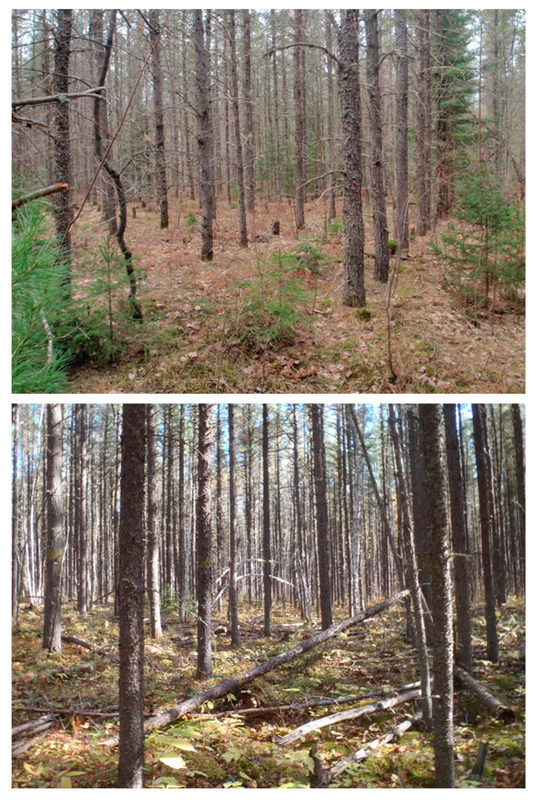
Figure 1. Contrasting high (bottom image; H) and low (top image; L) density-stressed semi-mature jack pine stands in central Canada: H is a 50 year-old natural-origin jack pine stand that was subjected to precommercial thinning at age 10; and L is a 35 year-old jack pine plantation subjected to initial spacing control at establishment. Note differences in tree sizes (diameter; L > H), branch diameter and development (L > H), inferred extractable solid wood HWPs (L > H), deadwood accumulation (H >> L), diameter distribution variation (H >> L), and positive skewness of diameter distribution (L >> H).
Forests 16 00610 g001
Figure 2. Species-specific cambial age prediction model (Equation (3)) residual plots: (a) raw residual–predicted value scatterplots; and (b) observed—predicted value scatterplots where the solid diagonal line denotes equivalency.
Forests 16 00610 g002
Figure 3. Species-specific exemplification of the SSDMM-generated whole-stem predicted values for the mean-sized tree (breast-height diameter = 22 cm) at rotation for the unthinned plantation (Regime 1): (a) stem height-specific cambial age predictions (Equation (3)); (b) height–diameter (taper) profiles with resultant cross-sectional diameter predictions; and (c) attribute predictions for the merchantable stem portion (stump to a 10 cm minimum top diameter). Note, attribute units for wood density, microfibril angle, modulus of elasticity, fibre coarseness, tracheid wall thickness, tracheid radial diameter, tracheid tangential diameter, and specific surface area are kg/m3, °, GPa, µg/m, µm, µm, µm, and m2/kg, respectively.
Forests 16 00610 g003
Figure 4. Temporal size–density trajectories for the three jack pine plantations growing under conditions consistent with a RCP4.5 climate change scenario on medium-to-good site qualities (SI = 18) situated in Northeastern Ontario (Kirkland Lake) as illustrated within the context of the traditional stand density management diagram (SDMD). Specifically, Regime 1 represented a crop plan that included a single initial espacement treatment consisting of the planting of 2400 genetically enhanced seedlings per hectare at an inter-tree spacing of 2.0 m × 2.0 m with no subsequent thinning treatments; Regime 2 represented a crop plan which included the identical initial espacement treatment as Regime 1 but in addition included a single heavy commercial thinning (CT) treatment at age 30 during which 35% of the basal area was removed; and Regime 3 represented a crop plan that likewise consisted of the identical initial espacement treatment as Regime 1 but also included two moderate CT treatments occurring at ages 30 and 45 during which 25% and 20% of the basal area was removed, respectively. Note, the SDMD graphically illustrates the following density-dependent relationships: (1) isolines for mean dominant height (Hd; parallel negative sloping solid lines progressing upwards from 4 m to 22 m by 2 m increments), quadratic mean diameter (Dq; parallel positive sloping dash lines progressing upwards from 4 cm to 26 cm by 2 cm increments), mean live crown ratio (Lr; parallel diagonal dashed lines demarking the 35% (outer-most), 40%, 50%, …, 80% (inner-most) values), relative density index (Pr; parallel diagonal short dashed lines progressing from 0.1 (inner-most) to 0.9 (outer-most) by 0.1 increments); (2) crown closure line (inner-most solid diagonal line); and self-thinning rule at a Pr = 1.0 (outer-most solid diagonal line); (3) lower and upper Pr isolines delineating the optimal density management window (Dm (0.32 ≤ Pr ≤ 0.45; pair of parallel diagonal short–long dashed lines); and (4) forecasted 65 year (2024–2089) size–density trajectories with 1 year intervals denoted for each regime. Refer to Table 1 for more detailed crop plan specifics.
Forests 16 00610 g004
Figure 5. Temporal size–density trajectories for the three red pine plantations growing under conditions consistent with a RCP4.5 climate change scenario on medium-to-good site qualities (SI = 23) situated in north-central Ontario (Thessalon) as illustrated within the context of the traditional stand density management diagram (SDMD). Specifically, Regime 1 represented a crop plan that included a single initial espacement treatment consisting of the planting of 2000 genetically enhanced seedlings per hectare at an inter-tree spacing of 2.2 m × 2.2 m with no subsequent thinning treatments; Regime 2 represented a crop plan which included the identical initial espacement treatment as Regime 1 but in addition included a single moderate-to-heavy commercial thinning (CT) treatment at age 40 in which 30% of the basal area was removed; and Regime 3 represented a crop plan that likewise consisted of the identical initial espacement treatment as Regime 1 but included two moderate CT treatments at ages 40 and 55 in which 20% of the basal area was removed during each intervention. Note, the SDMD graphically denotes (1) isolines for mean dominant height (Hd; parallel negative sloping solid lines progressing upwards from 6 m to 34 m by 2 m increments), quadratic mean diameter (Dq; parallel positive sloping dash lines progressing upwards from 4 cm to 40 cm by 2 cm increments), mean live crown ratio (Lr; parallel diagonal dashed lines demarking the 35% (outer-most), 40%, 50%, … 80% (inner-most) values), relative density index (Pr; parallel diagonal short dashed lines progressing from 0.1 (inner-most) to 0.9 (outer-most) by 0.1 increments); (2) crown closure line (inner-most solid diagonal line) and self-thinning rule at a Pr = 1.0 (outer-most solid diagonal line); (3) lower and upper Pr isolines delineating the optimal density management window (Dm (0.32 ≤ Pr ≤ 0.45; pair of parallel diagonal short–long dashed lines); and (4) forecasted 70 year (2024–2094) size–density trajectories with 1 year intervals denoted for each regime. Refer to Table 1 for more detailed crop plan specifics.
Forests 16 00610 g005
Figure 6. Interpretation guidance for the SSDMM-generated whole-tree 3-dimensional graphical representations (wood property maps) for cumulative attribute developmental patterns as exemplified for a mean-sized jack pine tree in terms of the Me attribute. Specifically, illustrating the cumulative value throughout the vertical and horizontal profiles of the main stem (i.e., 5 to 95 height percentiles by cambial age). The predicted values are contrasted at the 10 m height position when the tree was 52 and 65 years old. The resultant Me values of 11.4 and 13.0 reflect the overall wood stiffness of the entire cross-sectional disc at the 10 m stem height position at tree ages of 52 and 65, respectively. Hence both values are above the static-based Me threshold of 8.2 required for dimensional lumber status (sensu NLGA [20]). See text for additional inferences.
Forests 16 00610 g006
Figure 7. Exemplification of SSDMM-generated whole-tree 3-dimensional graphical representations of the cumulative attribute developmental patterns for the mean-sized jack pine tree (mean quadratic diameter; Dq) at rotation (65 yr) for the crop plan denoted Regime 1 (upper panel; Dq = 22 cm), Regime 2 (middle panel; Dq = 24 cm) and Regime 3 (lower panel; Dq = 26 cm) (Figure 4; Table 1): specifically, wafer plots for wood density, microfibril angle, and modulus of elasticity. Interpretation guidance for solid wood end-product inferences: contextual lumber grade class groupings for (1) low machine stress-rated (MSR) grade class grouping (1.2 E to 1.7 E) as defined by a Me value in the range of >8.3 to 12.1 GPa and a Wd value in the range of >400 to 440 kg/m3, (2) medium MSR grade class grouping (1.8 E to 1.9 E) as defined by a Me value in the range of >12.1 to 13.5 GPa and a Wd value in the range of >440 to 480 kg/m3, and (3) high MSR grade class grouping (2.0 E to 2.4 E) as defined by a Me value in the range of >13.5 to 16.5 GPa and a Wd value in the range of >480 to 520 kg/m3.
Forests 16 00610 g007aForests 16 00610 g007b
Figure 8. Exemplification of SSDMM-generated whole-tree 3-dimensional graphical representations of the cumulative attribute developmental profiles for the mean-sized red pine tree (mean quadratic diameter; Dq) at rotation (70 yr) for the crop plan denoted Regime 1 (upper panel; Dq = 22 cm), Regime 2 (middle panel; Dq = 28 cm) and Regime 3 (lower panel; Dq = 30 cm) (Figure 5; Table 1): specifically, wafer plots for wood density, microfibril angle, and modulus of elasticity. Refer to Figure 7 for interpretation guidance.
Forests 16 00610 g008aForests 16 00610 g008b
Table 2. Parameter estimates and associated statistics for species-specific cambial age models (Equation (3)).
Parameter orVariableParameter Estimate
Statistic Jack PineRed Pine
δ 00 -−1.27785713.914946
δ 01 D b ( k ) --
δ 02 H t ( k ) -0.135927
δ 03 A t ( k ) 1.0096100.772643
δ 10 H ( j k ) 0.851887−10.766666
δ 11 D b ( k ) H ( j k ) --
δ 12 H t ( k ) H ( j k ) --
δ 13 A t ( k ) H ( j k ) −0.0348580.102577
δ 20 H ( j k ) 2 −0.2670610.347923
δ 21 D b ( k ) H ( j k ) 2 0.001043-
δ 22 H t ( k ) H ( j k ) 2 0.0064800.002460
δ 23 A t ( k ) H ( j k ) 2 0.000961−0.005243
SEE a (yr) 1.0531.368
I2 b 0.9950.996
a Standard error of estimate (yr). b Index of fit.
Table 3. Exemplification of species-specific and spatially explicit mensurational and fibre attribute predictions for the mean-sized tree (quadratic mean diameter) at rotation by regime.
Species;
Crop Plan
[Db (cm); Ht (m)] a
Relative
Height
(%/100)
Stem
Height
(m)
[H]
Stem
Diameter
(cm)
[D] b
Cambial
Age c
(yr)
[A]
Attribute
Wd d
(kg/m3)
Ma d
(°)
Me d
(GPa)
Co d
(µg/m)
Wt d
(µm)
Dr d
(µm)
Dt d
(µm)
Sa d
(m2/kg)
Jack pine;0.071.220.563431.114.111.5412.42.7531.627.6307.9
Regime 10.162.918.760419.512.312.8407.12.7031.927.7315.8
[22; 17.7]0.264.617.656413.311.713.3399.72.6431.827.6321.4
0.366.416.553408.311.513.3392.12.5931.627.6326.2
0.468.115.248403.211.313.2384.92.5431.427.6330.5
0.569.813.544397.011.012.9379.12.4831.227.7334.7
0.6511.611.439388.810.612.5375.82.4231.028.0338.9
0.7513.38.734377.510.011.8376.52.3630.828.5343.5
0.8515.15.628360.59.510.4384.62.2930.629.4348.9
0.9516.82.022326.89.36.8420.02.1930.331.3356.1
Jack pine;0.061.222.363431.215.310.8416.02.7732.027.6304.7
Regime 20.163.120.359420.013.212.3409.62.7132.227.7312.8
[24; 18.9]0.264.919.156414.212.612.8401.52.6632.227.7318.4
0.366.818.052409.612.313.0393.12.6032.027.6323.2
0.468.716.648404.812.113.0385.12.5531.727.6327.5
0.5610.514.843399.111.712.9378.22.4931.527.7331.8
0.6512.412.538391.411.112.7373.52.4331.228.0336.3
0.7514.39.633380.710.312.3372.12.3731.028.4341.4
0.8516.16.127364.59.611.1376.92.2930.729.1347.9
0.9518.02.221332.49.37.7405.72.1930.330.7356.3
Jack pine;0.061.2224.1363430.616.810.0419.92.7832.427.7301.1
Regime 30.163.0921.9559420.014.311.6412.62.7232.627.8309.4
[26; 19.1]0.264.9720.6756414.313.612.2404.22.6732.627.7315.0
0.366.8419.4452409.913.212.5395.52.6232.427.7319.8
0.468.7217.9348405.312.812.6386.92.5632.127.7324.3
0.5610.5915.9743399.712.212.7379.22.5031.927.7328.9
0.6512.4713.4638392.211.412.8373.42.4431.627.9334.0
0.7514.3410.3533381.610.512.6370.82.3731.328.3339.9
0.8516.226.6327365.29.511.7374.42.2931.028.9347.3
0.9518.092.3621331.89.08.1402.82.1830.530.6357.0
Red pine;0.061.619.966442.110.017.0468.02.9832.630.3298.4
Regime 10.164.118.657425.28.817.0476.62.8533.131.2304.1
[22; 26.0]0.266.717.950404.09.316.4462.02.7233.631.0315.9
0.369.317.342385.310.415.6448.02.5934.130.7326.6
0.4611.916.535370.311.614.8436.22.4834.630.5335.2
0.5514.415.229358.912.714.1424.62.3735.030.3342.1
0.6517.013.424350.813.513.5410.22.2635.129.9348.0
0.7519.610.819346.014.013.0390.82.1634.629.4353.6
0.8522.17.314345.414.212.3364.22.0633.528.6359.6
0.9524.72.810355.713.411.8327.81.9631.127.3366.5
Red pine;0.061.625.366434.213.113.9480.52.9633.630.9295.9
Regime 20.164.223.657415.611.114.4489.12.8434.231.7301.8
[28; 26.6]0.266.822.849394.111.614.2474.32.7234.731.4313.7
0.369.522.142375.812.613.7460.22.6035.331.1324.3
0.4612.121.035361.213.813.1447.92.4935.730.9332.8
0.5514.719.429350.214.812.5435.22.3836.030.6339.5
0.6517.317.123342.215.511.9419.22.2836.030.3345.2
0.7520.013.818337.315.811.3397.52.1735.429.7350.5
0.8522.69.314336.415.710.6368.62.0734.028.8356.0
0.9525.23.511346.214.410.0330.01.9731.427.6362.0
Red pine;0.061.627.166432.814.113.2485.12.9534.031.1295.0
Regime 30.164.225.357413.611.913.8493.62.8434.531.9301.1
[30; 26.7]0.266.924.549391.912.313.7478.62.7235.131.6313.0
0.369.523.642373.613.313.2464.22.6035.631.3323.6
0.4612.222.535359.114.512.7451.72.4936.131.0332.0
0.5514.820.829348.015.512.1438.62.3936.330.7338.7
0.6517.418.323340.016.111.5422.12.2836.230.4344.3
0.7520.114.818334.916.410.9399.72.1835.629.8349.5
0.8522.710.014333.716.110.1370.02.0834.228.9354.8
0.9525.33.811343.214.69.5330.71.9731.527.6360.6
a Species-specific SSDMM-based predictions for the tree of mean quadratic diameter (Db; estimated by the Weibull-based parameter prediction equation system; [8] for jack pine, and [6] for red pine) and associated total tree height (Ht; estimated by the composite height–diameter function; [30] for jack pine, and [6] for red pine) at rotation for each regime. b Species-specific SSDMM-based predictions of upper stem inside bark diameter (D) at the specified stem height position (H) for the tree of mean quadratic diameter at rotation ( note, estimated using the embedded taper equations developed by Sharma and Parton [31] for jack pine and Sharma [32] for red pine). c Species-specific positional-based sectional cambial age prediction (A) for the tree of mean quadratic diameter at rotation as derived from Equation (3). d Species-specific positional-based predictions of Wd, Ma, Me, Co, Wt, Dr, Dt, and Sa which denote wood density, microfibril angle, modulus of elasticity, fibre coarseness, tracheid wall thickness, tracheid radial diameter, tracheid tangential diameter, and specific surface area, respectively, for the tree of mean quadratic diameter at rotation, as derived from Equation (5) in [7] when embedded into the SSDMMs.
Table 4. Rotational yield summaries and associated performance metrics for jack pine and red pine plantations managed according to crop plans outlined in Table 1.
Index aSpecies
(Unit)Jack PineRed Pine
ISIS + 1 CTIS + 2 CTsISIS + 1 CTIS + 2 CTs
Dq (cm)21.423.125.222.729.030.8
G (m2/ha)32.127.823.463.444.440.7
Vm(t) (m3/ha)-5035 + 35-10066 + 85
Vm(r) (m3/ha)244213183703500460
Vm (m3/ha)244263253703600611
Vt(t) (m3/ha)-5576-104156
Vt(r) (m3/ha)256223191722513472
Vt (m3/ha)256278267722617628
Vt(ca) (m3/ha)19854781068080
Nb (stems/ha)8916624781570675548
Nct (stems/ha)-1122851 + 311-1050753 + 415
Nca (stems/ha)1509616760430275284
R M A I ( V t ) (m3/ha/yr)3.94.24.110.38.89.0
R A M A I ( V t ) (m3/ha/yr)3.00.81.21.51.11.1
SS (m/m)8477761119091
RLEV-+2−5-+33+67
a Dq is predicted quadratic mean diameter at rotation; G is predicted stand-level basal area at rotation; V m ( t ) , V m ( r ) , and V m are predicted total merchantable volume extracted from thinnings, standing total merchantable volume at rotation, and total merchantable volume inclusive of thinning yields produced over rotation, respectively; V t ( t ) , V t ( r ) , and V t are predicted total volume extracted from thinnings, standing total volume at rotation, and total volume inclusive of thinning yields produced over the rotation, respectively; V t ( c a ) is the predicted total accumulated abiotic volume generated from self-thinning and non-density-dependent mortality events over rotation; Nb and Nct are total number of standing trees at rotation and total number of trees removed via thinning, respectively; Nca is total number of trees lost to mortality over rotation; R M A I ( V t ) and R A M A I ( V t ) are total stem volume-based mean annual biotic increment and total stem volume-based mean annual abiotic increment over rotation; Ss is rotational mean height/diameter ratio; and RLEV is land expectation value ratio (%) for thinning regimes relative to the unthinned regime.
Table 5. Rotational HWP summaries inclusive of SSDMM-generated wood quality attribute means and associated nominal grade classifications for jack pine plantations managed according to crop plans as outlined in Table 1 and graphically illustrated in Figure 4. Note, extractable HWPs are grouped into solid wood (SW) and non-solid wood (NSW) categories a.
Index bCrop Plan
(Unit)ISIS + 1 CTIS + 2 CTs
R @ 65CT1 @ 30R @ 65CT1 @ 30CT2 @ 45R @ 65
SWNSWSWNSWSWNSWSWNSWSWNSWSWNSW
Wd (kg/m3)413.4357.5402.1364413.4356.7401.3361409.5364.8414.4360
Ma (°)129.715.312129.714.811.71310.512.69.7
Me (GPa)12.59.210.28.112.59.210.47.911.6912.29.8
Co (µg/m)399.1402.7378.4398.2399.2403.1378.2405.5387.7403.6401400.2
Wt (µm)2.62.32.52.32.62.32.52.42.62.42.62.3
Dr (µm)31.430.132.63131.430.132.43131.530.531.630.4
Dt (µm)27.629.32829.927.629.32830.227.829.727.729.2
Sa (m2/kg)320.8346.4323342.9320.8346.4324.9343.5326.1344.5318.6345.7
GradeL-L-L-L-L-L-
Percent of volume
production
(m3/ha)
7822892802059558427921
a Solid wood (SW) and non-solid wood (NSW) classes for extractable HWPs are based on nominal grading-based attribute thresholds (NLGA [20]): SW HWP class includes all wood within merchantable stem sections that has minimum Wd and Me values of >400 kg/m3 and >8.2 GPa, respectively, whereas NSW HWP class includes all wood within merchantable stem sections that has Wd and Me values of ≤400 kg/m3 and ≤8.2 GPa, respectively. b Wd, Ma, Me, Co, Wt, Dr, Dt, and Sa denote wood density, microfibril angle, modulus of elasticity, fibre coarseness, tracheid wall thickness, tracheid radial diameter, tracheid tangential diameter, and specific surface area, respectively. Grade denotation L is the nominal solid wood dimensional lumber-based grade for the low quality class as inferred from Wd and Me thresholds (NLGA [20]): low grade dimensional lumber (1.2 E to 1.7 E) defined as 400 < Wd (kg/m3) ≤ 440 and 8.3 < Me (GPa) ≤ 12.1.
Table 6. Rotational HWP summaries inclusive of SSDMM-generated wood quality attribute means and associated nominal grade classifications for red pine plantations managed according to crop plans outlined in Table 1 and graphically illustrated in Figure 5. Note, extractable HWPs are grouped into solid wood (SW) or non-solid wood (NSW) categories a.
Index bCrop Plan
(Unit)ISIS + 1 CTIS + 2 CTs
R @ 70CT1 @ 40R @ 70CT1 @ 40CT2 @ 55R @ 70
SWNSWSWNSWSWNSWSWNSWSWNSWPSWNSW
Wd (kg/m3)422.7448362.2-331.5423.2354.8-331.5-340.2376.5424.3352.8
Ma (°)9.38.112.6-14.211.914.3-14.2-16.615.412.614.6
Me (GPa)1720.213.8-21.614.412.1-21.6-14.711.913.911.8
Co (µg/m)469.8461.8404.2-402.4483.3415.5-402.4-385.7469.5486.8414.3
Wt (µm)2.832.3-2.12.92.3-2.1-2.22.62.92.3
Dr (µm)33.13234-40.633.934.8-40.6-36.53634.134.9
Dt (µm)3130.129.6-29.631.330-29.6-28.931.431.430
Sa (m2/kg)307.3301.6345.1-389.2300.3340.9-389.2-375.1319.4298.5340.9
Lumber gradeLM---L------L-
Percent of volume
production
(m3/ha)
93259-1003466-100-10093061
a Solid wood (SW) and non-solid wood (NSW) classes for extractable HWPs as defined in Table 5 footnotes. P denotes the pole HWP class. b Wd, Ma, Me, Co, Wt, Dr, Dt, and Sa as defined in Table 5 footnotes. Grade denotations L and M are nominal solid wood dimensional lumber-based grades for low and medium quality classes as inferred from Wd and Me thresholds (NLGA [20]): low grade dimension lumber (1.2 E to 1.7 E) defined as 400 < Wd (kg/m3) ≤ 440 and 8.3 < Me (GPa) ≤ 12.1 whereas medium grade dimensional lumber (1.8 E to 1.9 E) defined as 440 < Wd (kg/m3) ≤ 480 and 12.1 < Me (GPa) ≤ 13.5.
Disclaimer/Publisher’s Note: The statements, opinions and data contained in all publications are solely those of the individual author(s) and contributor(s) and not of MDPI and/or the editor(s). MDPI and/or the editor(s) disclaim responsibility for any injury to people or property resulting from any ideas, methods, instructions or products referred to in the content.