Prediction and Trade-Off Analysis of Forest Ecological Service in Hunan Province on Explainable Deep Learning

Abstract

Ecosystem services play a crucial role in maintaining ecological balance, providing essential functions. This study examines the trade-offs and synergies among five key ecosystem services in ecological forests across different regions of Hunan Province, China. Various machine learning models are compared to predict ecosystem service value (ESV) levels, with the most effective predictive model identified. The SHAP (SHapley Additive exPlanations) analysis is employed to identify key environmental and management factors influencing ecosystem services. Our findings reveal significant regional variations in ecosystem services, with the eastern and western regions showing superior soil conservation and forest nutrient retention. In contrast, the southern and western regions, particularly karst areas, display fewer trade-offs between ecosystem services, likely due to the effectiveness of ecological policies. SHAP analysis further reveals that factors such as precipitation during the warmest quarter, central government compensation funds, and timber harvesting volume strongly influence regional ESV. This study provides valuable insights for improving ecosystem service management and policy-making in rapidly developing regions, underscoring the importance of ecological protection strategies for sustainable development.

1. Introduction

The importance of ecosystem services in preserving ecosystem equilibrium is paramount, offering key amenities to nature and the natural world alike such as storing carbon, protecting soil, purifying water, and conserving biodiversity. These services play a pivotal role in life on Earth [1,2]. Yet, with ongoing human impacts on the environment, calculating and forecasting ecosystem service values (ESVs) are increasingly significant, especially for efficient environmental management and decision-making [3,4]. The Hunan Province, celebrated for its abundant natural forest resources and varied ecosystems, forms an essential segment of China’s forest ecosystems. As crucial in Hunan’s ecological protection framework, ecological forests provide numerous services like climate control and conservation, and are vital for sustaining regional ecological stability and protection. The importance of ecological forests has expanded, particularly because timber harvesting is not the main management focus. Their diverse ecological services, including regulating climate and conserving water, have attracted heightened focus [5].

As Hunan undergoes rapid urbanization and industrialization, understanding the mechanisms driving ecosystem services is key to achieving sustainable development [6]. Recently, research has intensely focused on the balance and cooperation among ecosystem services [7,8]. Enhancing one service often results in the degradation of another due to resource scarcity rivalry [9]. Conversely, synergies are scenarios where improving one service can concurrently lead to the betterment of other services. Comprehending these dynamics is vital for effective land utilization adjustments and ecological rejuvenation endeavors, given their varied and sometimes conflicting effects on ecosystems [10]. For instance, while afforestation can boost carbon storage, its lack of appropriate management might adversely affect the local water cycle balance [11]. Consequently, a thorough evaluation of ecosystem service compromises provides scientific proof for swiftly evolving areas, aiding in making decisions about environmental conservation and regional growth [12].

The grasp of ecosystem service value is still not fully developed due to its intricate and evolving interplay among various service types [13,14,15]. The interplay of ecosystem service value in different areas, both spatially and annually, shaped by variables like climate, landscape, and land use, continues to be ambiguous [16,17,18,19], making its real-world implementation more difficult. The challenge, especially due to climate change and human activities, lies in finding a complex web of interplay between complex, multi-faceted ecosystem services, with inadequate research on their compensatory impacts [20]. The swift advancement of deep learning and machine learning technologies has led to a rise in the use of interpretable deep learning methods to evaluate and predict the worth of various ecosystem services [21]. Integrating diverse data sources in these approaches uncovers complex non-linear connections and offers a profound understanding of these underlying factors. For instance, Reichstein et al. employed machine learning models to forecast shifts in ecosystem service values in the Qinghai-Tibet Plateau in various contexts [22]. Li et al. (2025) utilized machine learning models to assess and predict the ecosystem service value in the Yunnan-Guizhou Plateau, identifying land use changes and vegetation cover as the primary driving factors and proposing the optimal management strategy under an ecological priority scenario [23]. Das et al. (2021) combined machine learning algorithms with the CA-Markov model to evaluate and predict the ecosystem service value in a region of Asia, emphasizing the advantages of machine learning in handling complex ecological data [24]. Additionally, Hossain et al. (2024) used artificial neural networks to predict the impact of land use changes on the ecosystem service value, providing scientific guidance for land planning and management [25]. Nonetheless, most existing studies depend on standard ecosystem service evaluations, overlooking key ecological aspects like the unique drivers of climate change [26] and important factors like forest management. Moreover, while many machine learning models exist, each with its own characteristics and suitable application scenarios, selecting the appropriate model for simulation remains a significant challenge. Furthermore, in many studies, the “black-box” nature of machine learning models results in poor interpretability and transparency of simulation outcomes, which significantly impacts the application of machine learning in ecosystem service value (ESV) estimation models. Thus, more accurate models for analyzing the ecosystem service value loss in the context of ecosystem service processes are crucial for Hunan’s welfare evolution in guiding the scientific formulation of regional ecological protection policies.

Lately, there has been considerable advancement in the development of ecosystem service forecasting and modeling, where machine learning has gained prominence as an effective means for precise predictions with substantial, intricate datasets. Numerous investigations have focused on employing machine learning methods, including random forests, support vector machines, and gradient boosting models, for estimating ecosystem service values [27]. However, the notable improvements in predictive accuracy notwithstanding machine learning techniques frequently struggle with clarity and comprehensibility [28,29]. This study addresses these gaps by focusing on Hunan Province. As such, our research aims at the following objectives: 1. Examine the trade-offs and synergies among ecosystem services across Hunan’s distinct ecological regions, with a focus on soil conservation, water source conservation, carbon sequestration, forest nutrient retention, and air purification. 2. Develop an explainable machine learning framework to predict ESV levels (low, medium, high) by integrating bioclimatic factors and forest management variables, with a focus on identifying key drivers of ESV using SHAP analysis.

2. Materials and Methods

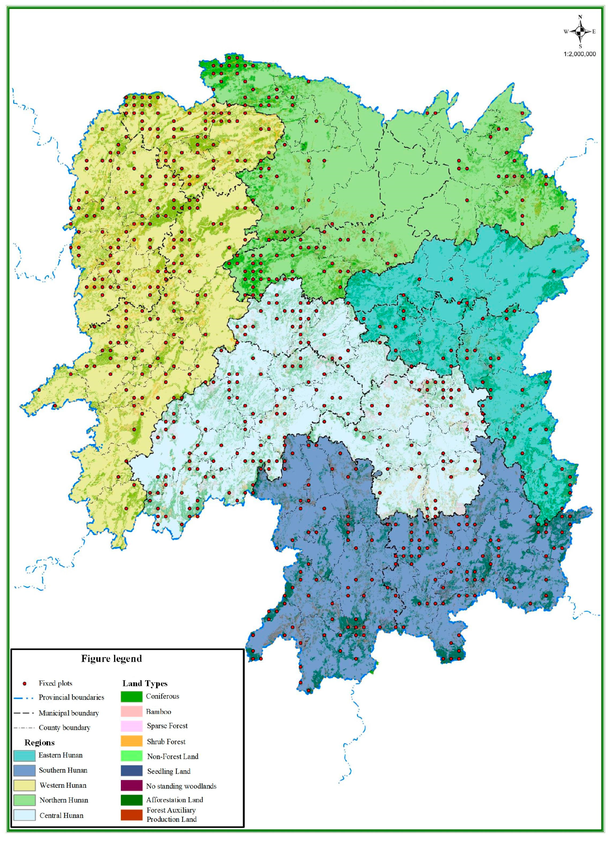
2.1. Data Sources

Our study targets ecological forests, which are forests that maintain ecosystem service functions situated in Hunan Province, China. These forests represent the most significant forest resource in Hunan, covering 36.65% of the total forest area, and are highly protected. The data used in this study are derived from monitoring data collected from 683 long-term fixed monitoring plots of 1000 m² in the ecological forests range of Hunan Province (Figure 1, updated in 2019) [30]. These plots are evenly distributed across all counties and districts in Hunan Province (except for Furong District, Kaifu District, Shigu District, and Zhengxiang District, where no ecological forests are distributed). The plots cover various vegetation types, river basins, and ecological locations.

In order to further analyze the influencing factors of ecosystem service value, we also obtained 24 related environmental and management variables (

Table 1. Nineteen bioclimatic and five forest resource management variables.

	Code	Description
Bioclimatic variables	bio1	Annual mean temperature
	bio2	Mean diurnal range (mean of monthly (max temp. − min temp.))
	bio3	Isothermality (bio2/bio7) (×100)
	bio4	Temperature seasonality (standard deviation × 100)
	bio5	Max temperature of warmest month
	bio6	Min temperature of coldest month
	bio7	Temperature annual range (bio5–bio6)
	bio8	Mean temperature of wettest quarter
	bio9	Mean temperature of driest quarter
	bio10	Mean temperature of warmest quarter
	bio11	Mean temperature of coldest quarter
	bio12	Annual precipitation
	bio13	Precipitation of wettest month
	bio14	Precipitation of driest month
	bio15	Precipitation seasonality (coefficient of variation)
	bio16	Precipitation of wettest quarter
	bio17	Precipitation of driest quarter
	bio18	Precipitation of warmest quarter
	bio19	Precipitation of coldest quarter
Forest Resource Management variables	E1	Bamboo harvesting volume
	E2	Timber harvesting volume
	E3	Area of ecological forests
	E4	Central government compensation funds
	E5	Provincial government matching compensation funds

). We first obtained five forest resource management variables for each region’s ecological forests from the Forestry Bureau of Hunan Province. These factors include the bamboo harvesting volume, timber harvesting volume, area of ecological forests, central government compensation funds, and provincial government matching compensation funds. Additionally, 19 biologically meaningful variables (bioclimatic variables) for each plot were extracted from WorldClim (http://www.worldclim.org/, accessed on 10 April 2024). All factors are listed in Table 1.

2.2. Quantification of Ecological Services

The data for the assessment of ecological services in Hunan Province’s forests were derived from the fixed plot survey data within each county [31], and were then combined with the observation data from the ecological stations for calculation (based on the [32]) to determine the ecological service value for each county. These forest ecological stations are predominantly managed by the National Forestry and Grassland Administration and provided datasets that supported the assessment. This research concentrated on five distinct forest ecosystem activities: conservation of water sources (10,000 tons each year), soil preservation (10,000 tons annually), carbon capture and oxygen discharge (10,000 tons annually), forest nutrient preservation (10,000 tons annually), and air cleansing (10,000 tons per year). The assessments were carried out independently for each of these functions, with comprehensive indicator systems and corresponding formulas detailed in the reference [32]. To convert the values for the ecosystem service function evaluation of Hunan’s ecological forests, the equivalent substitution method was used. This method necessitated incorporating social public information sourced from pertinent national and local Hunan departments (see Appendix A;

Table A1. Public social data on forest ecosystem service evaluation in Hunan Province.

Name	Unit	Evaluation Reference Price	Source and Basis
Reservoir Construction Unit Reservoir Investment	RMB/ton	9.79	Based on the average reservoir investment cost of 2.17 RMB/ton from the “China Water Resources Yearbook”, adjusted using the 2012 price index of raw materials, fuel, and power published by the National Bureau of Statistics, resulting in a 2012 unit reservoir cost of 8.08 RMB/ton, then adjusted to the present price using a discount rate.
Water Purification Cost	RMB/ton	3.56	The average residential water price in major cities in China in 2012 was 3.07 RMB/ton, obtained by the grid method, then adjusted to the present price using the discount rate.
Excavation Cost per Unit Area of Earthwork	RMB/cubic meter	73.08	Based on “Water Conservancy Engineering Budget Norms (Volume 1)” published by the Yellow River Water Conservancy Press in 2002, the labor cost for digging I and II type soils requires 42 man-hours per 100 cubic meters, with a labor cost of 150 RMB/day, adjusted to 73.08 RMB/cubic meter in the present year.
Ammonium Dihydrogen Phosphate Nitrogen Content	%	14	Fertilizer product specification.
Ammonium Dihydrogen Phosphate Phosphorus Content	%	15.01
Potassium Chloride Potassium Content	%	50
Ammonium Dihydrogen Phosphate Fertilizer Price	RMB/ton	3828	Prices of ammonium dihydrogen phosphate and potassium chloride fertilizers were adjusted to the present price based on the average spring price in 2012 from the China Fertilizer Network (http://www.fert.cn, accessed on 10 April 2024). Organic material prices were adjusted to the present price based on the average spring price of chicken manure organic fertilizer from the China Agricultural Materials Network (www.ampcn.com, accessed on 10 April 2024) at the end of the 12th Five-Year Plan.
Potassium Chloride Fertilizer Price	RMB/ton	3248
Organic Material Price	RMB/ton	928
Carbon Sequestration Price	RMB/ton	1485.96	Based on the 2006 CO2 market price of 31 EUR/ton from the EU CO2 market, adjusted to the present price using a discount rate.
Oxygen Manufacturing Price	RMB/ton	1506.92	Based on the average spring price of oxygen in 2007 from the Ministry of Health of the People’s Republic of China (http://www.nhc.gov.cn/, accessed on 10 April 2024), adjusted to the present price using a discount rate.
Negative Ion Production Cost	RMB/1018 units	10.97	According to the applicable range of the KLD-2000 ion generator, which is 30 square meters (with a room height of 3 m), a power of 6 watts, a negative ion concentration of 1,000,000 ions per cubic meter, a service life of 10 years, and a price of 65 Yuan each, the negative ion lifespan is 10 min. By the end of the 12th Five-Year Plan, the electricity rate is 0.65 Yuan per kWh. The cost of generating negative ions is calculated to be 9.46 Yuan per 1018 ions, and the discounted price is 10.97 Yuan per 1018 ions.
Sulfur Dioxide Treatment Cost	RMB/kg	2.15	Based on the pollution fee standards in the 31st order from the National Development and Reform Commission and four other ministries in 2003, adjusted to the present price using a discount rate.
Fluoride Treatment Cost	RMB/kg	1.23
Nitrogen Oxide Treatment Cost	RMB/kg	1.13
Lead and Lead Compound Pollution Treatment Cost	RMB/kg	53.55
Cadmium and Cadmium Compound Pollution Treatment Cost	RMB/kg	35.69
Nickel and Nickel Compound Pollution Treatment Cost	RMB/kg	8.25
Tin and Tin Compound Pollution Treatment Cost	RMB/kg	3.97
Dust Cleaning Cost	RMB/kg	0.27
PM10 Cleaning Cost	RMB/kg	2.03	Based on the equivalent values of carbon black dust pollution and taxable pollution in Hunan Province.
PM2.5 Cleaning Cost	RMB/kg	2.03
Windproof and Sand Fixation Ecological Subscription Price	RMB/(hectare per year)	7647.88	The funding amount for desert reclamation in 2002 was 5000 RMB/(hectare per year) as per the paper “Design and Operation Channels of the Ecological Purchase in the Shaanxi-Gansu-Ningxia Border Area.” This amount was then adjusted to the ecological subscription price using the industrial producer price index, resulting in an ecological subscription price of 7647.88 RMB/(hectare per year), adjusted to the present price using the industrial producer price index.
Crop and Pasture Price	RMB/kg	2.32	Based on the average price at the end of the 12th Five-Year Plan from the New Agricultural Materials Network (www.xnynews.com/quote/list-297.html, accessed on 10 April 2024), discounted to the present price.

). Subsequently, the values for each of the five forest ecosystem functions per area unit were computed for every county and district.

2.3. Calculation of Trade-Offs

The data collected from Hunan Province are divided into five ecological regions: Eastern Hunan, which includes Changsha, Zhuzhou, and Xiangtan; Southern Hunan, which includes Chenzhou and Yongzhou; Western Hunan, which includes the Xiangxi Tujia and Miao Autonomous Prefecture, Huaihua, and Zhangjiajie; Northern Hunan, which includes Changde, Yueyang, and Yiyang; and Central Hunan, which includes Hengyang, Loudi, and Shaoyang.

The compromises involving two ecosystem functions indicate their direct interplays, whereas the compromises across various ecosystem services are more intricate [33]. Hence, we analyzed the compromises in ten different pairings of these services. The Root Mean Square Deviation (RMSD) is a frequently utilized statistical measure to gauge the extent of these trade-offs among ecosystem services [34,35]. To normalize the advantages of each ecosystem service, unit variances were removed using the Min-Max Normalization approach prior to computing the RMSD [35].

The RMSD was calculated as follows:

$$\begin{array}{l}\\ \mathrm{RMSD}=\sqrt{{\displaystyle \frac{1}{\mathrm{n}-1}}\cdot {{\displaystyle \sum _{\mathrm{i}=1}^{\mathrm{n}}({\mathrm{ES}}_{\mathrm{i}}-{\mathrm{ES}}_{\exp })}}^2}\\ \end{array}$$

(1)

where ES_i represents the standardized value of the i-th ecosystem service, and ES_exp is the expected value of the i-th ecosystem service. In comparing the magnitude of trade-offs between any two ecosystem services, their RMSD value indicates the deviation from the 1:1 line of equal benefit. A larger angle with the vertical axis, relative to the horizontal axis, suggests that the ecosystem services represented by the horizontal axis are more beneficial, and vice versa. Additionally, the greater the angle between the spikes and the 1:1 line, the higher the trade-offs between the paired ecosystem services, assuming the lengths of the spikes are identical.

2.4. Prediction of Ecological Service Value Levels Based on the Machine Learning Method

The ecological valuation for every area in each county/district was segmented into three categories: high (exceeding 120,000 Yuan per hectare), medium (ranging from 100,000 to 120,000 Yuan per hectare), and low (under 100,000 Yuan per hectare). Utilizing this categorization, we formulated a predictive model for ecological significance and feature prediction employing XGBoost (R 4.4.1) [36], predicting the ESV levels based on biological environmental factors and forest management factors. Data preprocessing entailed processing missing data, detecting anomalies, and normalizing missing data. The approach of the model’s values applied the median and filtering of the interquartile range method to fill them. To resolve discrepancies between features, all numerical aspects were normalized. Beyond XGBoost, we utilized five other machine learning techniques: Logistic Regression, k-Nearest Neighbors (NN), Linear Analysis, Decision Tree, Random Forest, LightGBM and Vector Support Machine (SVM), and conducted a performance comparison of the XGBoost. Each model’s performance was cross-validated and tested against the model’s performance.

A thorough evaluation of each model’s effectiveness involved utilizing classification metrics like accuracy, precision, recall, F1 score, and AUC. Given that ecological value classification involves three classes, the One-vs-Rest (OvR) method was implemented to determine the multi-class AUC. Accuracy, as the primary evaluation metric, reflects the proportion of accurately predicted samples relative to the total sample count. Precision, concentrates on the rate of correctly anticipated positive samples within a positive category. Conversely, Recall focuses on the actual sample count, the ratio of correctly predicted positive samples among accurately predicted positive ones. The F1 score merges both precision and recall, varying from 0 to 1. A score of 1 indicates the superior model output, but 0 denotes the least successful one.

Hyperparameter tuning for the LightGBM model was performed using a grid search. For a deeper insight into how various ecological environmental elements affect the prediction of ecological values, SHAP (SHapley Additive exPlanations) was employed. The SHAP measurements assess how much each characteristic affects the model’s output, aiding in recognizing crucial elements that shape the classification of ecological values, and thus improving the model’s clarity.

3. Results

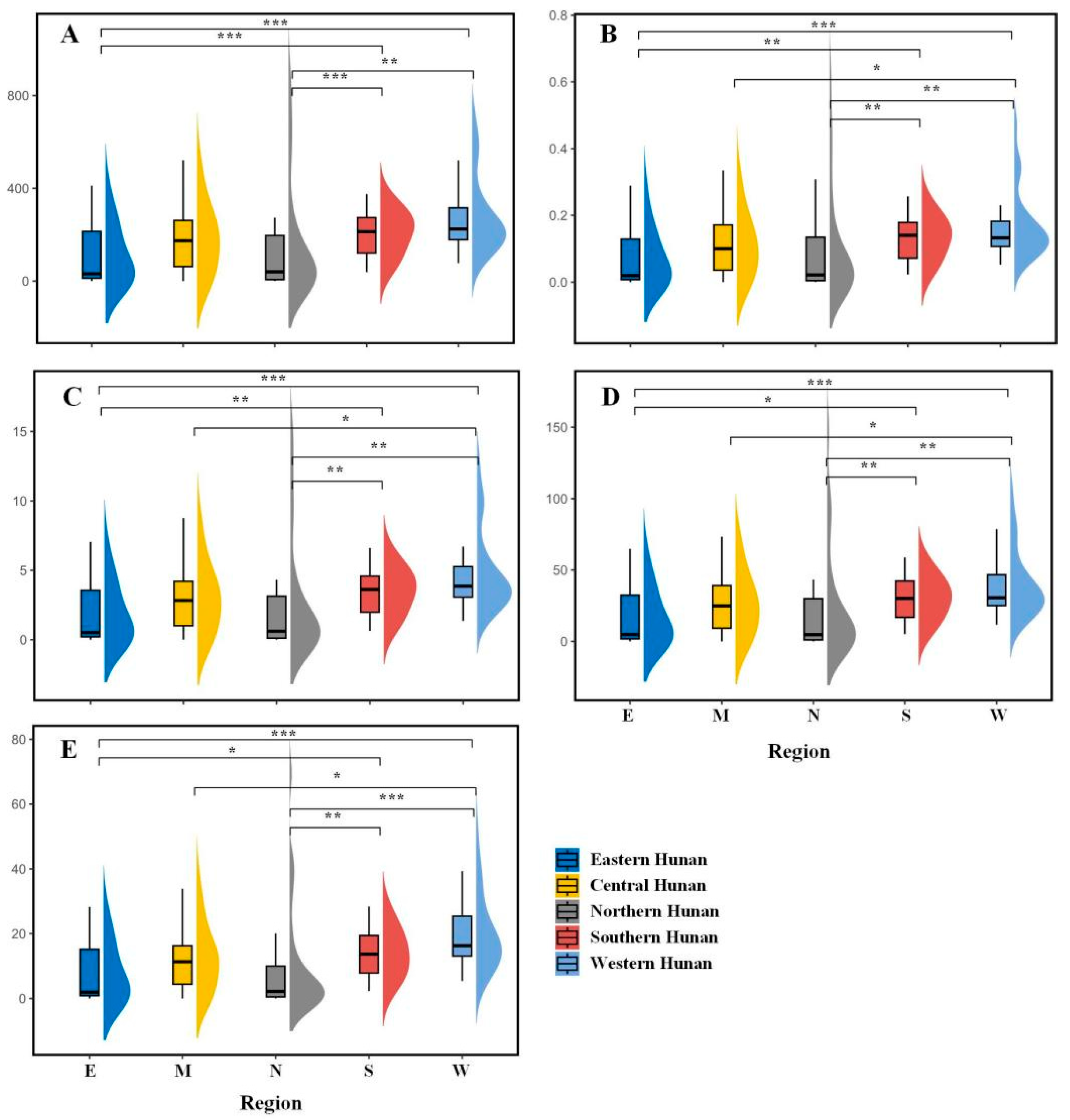
3.1. Quantification of Ecological Services

The comparison of ecological services across different regions revealed significant differences of five ecosystem services. For soil, conservation (Figure 2A) varied significantly between regions, with the eastern and western regions showing higher levels of soil conservation compared to the northern and southern regions (p < 0.05). Similarly, forest nutrient retention (Figure 2B) was higher in the eastern, southern, and western regions compared to the northern region (p < 0.01). In terms of water source conservation (Figure 2C), the western region showed the highest values, with significant differences between regions (p < 0.05). For carbon sequestration and oxygen release (Figure 2D), the southern region had the greatest benefit, with significant differences observed (p < 0.001). Lastly, air purification (Figure 2E) was highest in the eastern region (p < 0.05).

3.2. Trade-Offs Between Ecological Indicators

The scatter-plot matrices presented in Figure 3 illustrate the trade-offs between paired ecological indicators (standardized values) across the five regions, with special emphasis on the entire region. The results highlight significant regional variation in the relationships between ecological services, with each region exhibiting unique patterns of trade-offs.

In the entire region, trade-offs were observed between soil conservation (SC)-forest nutrient retention (FN), water source conservation (WS)-carbon sequestration (CO), water source conservation (WS)-air purification (AP), SC-CO, SC-AP, FN-AP, and WS-AP. In Eastern Hunan and Western Hunan, the trade-offs between SC-FN and FN-AP pairs were observed. In Southern, Northern, and Central Hunan, the trade-offs between AP and others were observed.

The root mean square deviation (RMSD) values for the paired trade-offs among ecological services (ESs) across six regions are summarized in

Table 2. Root mean square deviation (RMSD) values of the paired trade-offs among six regions. Soil conservation: SC; forest nutrient retention: FN; water source conservation: WS; carbon sequestration and oxygen release: CO; air purification: AP.

Regions	Paired ES Trade-Offs	FN	WS	CO	AP
Eastern Hunan	SC	0.042	0.011	0.017	0.027
Southern Hunan		0.049	0.033	0.052	0.087
Western Hunan		0.051	0.023	0.034	0.041
Northern Hunan		0.027	0.012	0.040	0.077
Central Hunan		0.032	0.018	0.034	0.064
The entire region		0.032	0.011	0.040	0.050
Eastern Hunan	FN		0.036	0.034	0.059
Southern Hunan			0.031	0.029	0.070
Western Hunan			0.033	0.027	0.055
Northern Hunan			0.027	0.026	0.068
Central Hunan			0.028	0.045	0.067
The entire region			0.032	0.018	0.041
Eastern Hunan	WS			0.010	0.027
Southern Hunan				0.035	0.065
Western Hunan				0.024	0.039
Northern Hunan				0.038	0.072
Central Hunan				0.034	0.050
The entire region				0.039	0.047
Eastern Hunan	CO				0.027
Southern Hunan					0.059
Western Hunan					0.036
Northern Hunan					0.045
Central Hunan					0.061
The entire region					0.028

. The lower values suggest stronger alignment between the paired services and higher values suggest more significant trade-offs.

In Southern Hunan, the SC-FN trade-off had a higher RMSD of 0.049, indicating a greater conflict between soil conservation and nutrient retention compared to other regions. The trade-offs between SC and CO, as well as SC and AP, had RMSD values of 0.052 and 0.087, respectively, suggesting significant trade-offs. Southern Hunan exhibited some of the highest RMSD values, particularly in the AP trade-off, highlighting more substantial conflicts in ecological service interactions. For Western Hunan, the trade-off between SC and FN had an RMSD value of 0.051, while the SC-CO and SC-AP trade-offs showed RMSD values of 0.034 and 0.041, respectively. These values indicate moderate to high trade-offs between soil conservation and carbon sequestration or air purification. Similarly, the CO and AP trade-off in Western Hunan had an RMSD value of 0.041, signaling a mild but notable trade-off. In Northern Hunan, the SC-FN trade-off had the lowest RMSD value (0.027), reflecting a relatively harmonious relationship between soil conservation and nutrient retention. However, the SC-CO and SC-AP trade-offs showed higher RMSD values of 0.040 and 0.077, respectively, indicating notable trade-offs. The CO and AP trade-off was also relatively high (0.045), indicating a clear conflict between these two services. In Central Hunan, the SC-FN and SC-CO trade-offs had RMSD values of 0.032 and 0.034, respectively, suggesting mild trade-offs. However, the SC-AP trade-off in Central Hunan had a significantly higher RMSD of 0.064, reflecting a more substantial trade-off between these services. Similarly, the CO and AP trade-off had a higher RMSD value of 0.061.

For the entire region, the overall RMSD values across the various trade-offs were generally lower. The SC-FN trade-off had an RMSD of 0.032, SC-WS 0.011, and SC-CO 0.040, indicating relatively lower conflicts in the entire region. The CO-AP trade-off in the entire region showed an RMSD value of 0.050, which is moderate but suggests a more balanced relationship between carbon sequestration and air purification compared to the other regions.

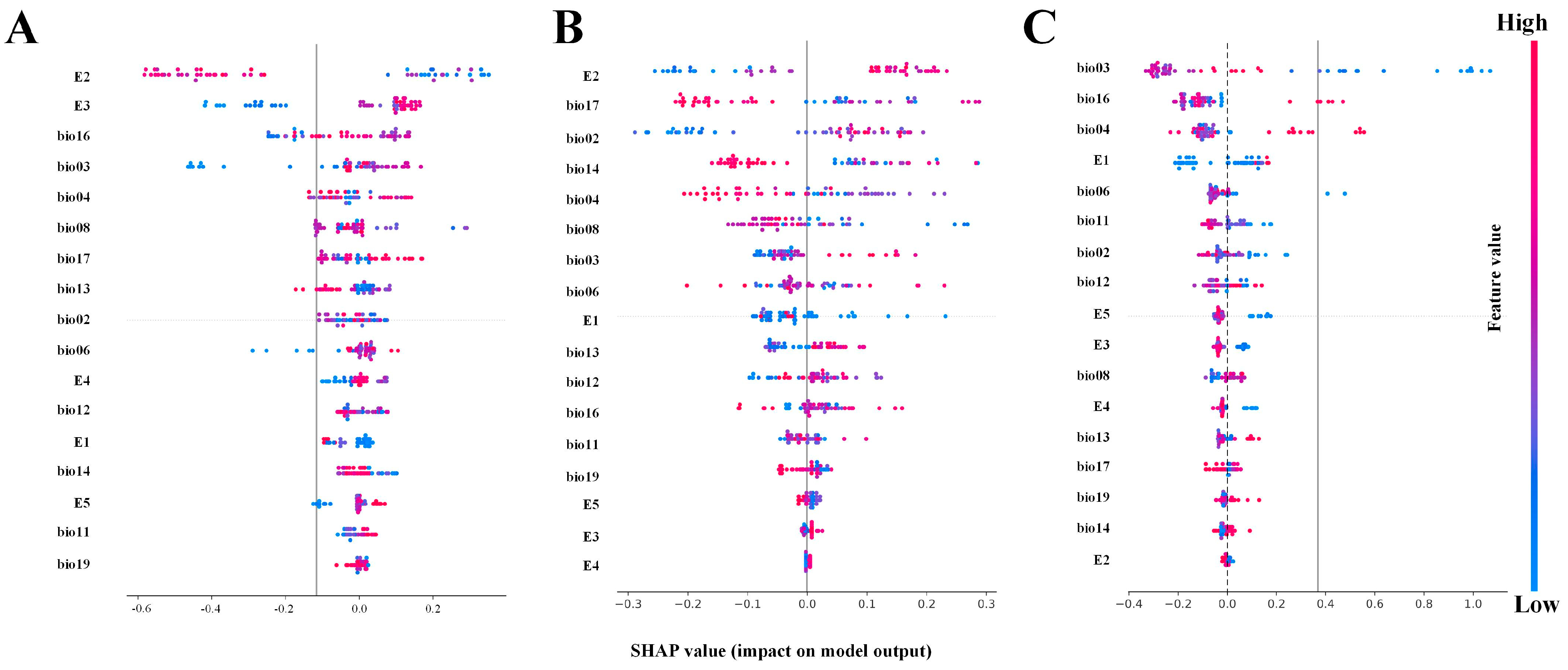
3.3. Fitting Machine Learning Models for Ecological Service Value Prediction

Figure 4A presents the complete correlation matrix of 19 bioclimatic factors. The heatmap reveals several strong correlations between variables with many showing high correlations (dark blue and red cells with values close to 1 and −1) indicating redundant information. Variables like bio01, bio05, and several others show particularly strong correlation patterns with multiple factors. Figure 4B displays the refined correlation matrix after removing highly correlated environmental factors, resulting in a significantly simplified matrix with fewer variables that show more moderate correlation values overall, while key variables like bio12, bio19, and bio06 have been retained. This refined matrix likely represents a more efficient set of predictors for machine learning models, reducing multicollinearity problems while preserving important environmental information for modeling purposes.

By comparing the learning curves of different machine learning algorithms (Figure 4C–I), LightGBM demonstrated the best performance in all tests, particularly in cross-validation scores, which were significantly higher than those of the other five algorithms. This indicates that LightGBM has superior generalization ability for ecological service value prediction tasks. Both Random Forest and SVM showed a similar performance, with their cross-validation scores fluctuating, but they still exhibited relatively good generalization performance. In contrast, Logistic Regression and k-Nearest Neighbors (KNNs) models showed more pronounced overfitting during training, with lower cross-validation scores.

Table 3. Performance comparison of different models.

Model	Precision	Recall	F1 Score	AUC	Cross-Validation
Logistic Regression	0.66	0.72	0.69	0.70	0.61
k-Nearest Neighbors	0.68	0.72	0.70	0.77	0.58
Decision Tree	0.55	0.48	0.51	0.53	0.55
Random Forest	0.61	0.68	0.64	0.69	0.59
SVM	0.62	0.72	0.64	0.66	0.62
LightGBM	0.66	0.72	0.69	0.71	0.58
XGBoost	0.69	0.72	0.70	0.69	0.55
After Hyperparameter Optimization
Logistic Regression	0.66	0.72	0.69	0.70	0.64
k-Nearest Neighbors	0.68	0.72	0.70	0.77	0.63
Decision Tree	0.58	0.44	0.50	0.55	0.59
Random Forest	0.54	0.64	0.58	0.67	0.58
SVM	0.62	0.72	0.64	0.65	0.62
LightGBM	0.66	0.72	0.69	0.71	0.65
XGBoost	0.69	0.72	0.7	0.69	0.62

shows the performance comparison of different models based on precision, recall, F1 score, AUC, and cross-validation score. Before optimization, k-Nearest Neighbors (KNNs) performed the best, with a precision of 0.68, recall of 0.72, F1 score of 0.7, and AUC of 0.77, though its cross-validation score was 0.58. Logistic Regression showed balanced results with a precision of 0.66, recall of 0.72, and F1 score of 0.69, but its AUC of 0.7 indicated room for improvement. The Decision Tree model had the lowest performance across most metrics, with a precision of 0.55 and AUC of 0.53. Random Forest and SVM also showed a moderate performance, with Random Forest achieving a precision of 0.61 and SVM having a balanced recall of 0.72. LightGBM showed a strong performance, with an AUC of 0.71, though its cross-validation score was low at 0.58. XGBoost had a good precision of 0.69, but its cross-validation score of 0.55 suggested a weaker generalization. After hyperparameter optimization, k-Nearest Neighbors and Logistic Regression maintained a strong performance, with KNN continuing to have the highest AUC of 0.77. Decision Tree’s performance slightly improved, but it still remained one of the weakest models. Random Forest and SVM showed slight improvements, with Random Forest’s precision decreasing to 0.54, while SVM’s performance remained steady. LightGBM’s performance improved, with a higher cross-validation score of 0.65. XGBoost’s results remained consistent, with good precision and recall.

Based on the above analysis, XGBoost is selected as the optimal model due to its superior performance in handling complex datasets and non-linear relationships. Specifically in this analysis, XGBoost performed exceptionally well across multiple metrics, including precision, recall, and F1 score. XGBoost is a tree-based ensemble learning model, and the SHAP analysis is particularly well-suited for explaining tree models. The feature importance in tree models is generally intuitive, clearly demonstrating the contribution of each feature to the prediction outcome. Compared to other models, the SHAP analysis for XGBoost is more computationally efficient, making it the preferred model for handling large-scale datasets. Therefore, XGBoost not only excels in terms of model performance, but also provides profound interpretability through SHAP analysis, offering crucial support for further optimization and decision-making.

Table 4. Best parameters of seven models after hyperparameter optimization.

Models	Parameter Name	Parameter Explanation	Best Parameter
Logistic Regression	C	Regularization strength parameter	0.1
	max_iter	Maximum iterations	200
	solver	Algorithm selection for optimization problem	liblinear
k-Nearest Neighbors	metric	Distance metric	euclidean
	n_neighbors	Number of neighbors	7
	weights	Assign weights	uniform
Decision Tree	max_depth	Maximum depth	5
	min_samples_leaf	Minimum samples per leaf	4
	min_samples_split	Minimum samples per split	2
Random Forest	max_depth	Maximum depth	3
	min_samples_leaf	Minimum samples per leaf	1
	min_samples_split	Minimum samples per split	5
	n_estimators	The number of boosting iterations	300
SVM	C	Regularization strength parameter	1
	gamma	Regularization parameter	scale
	kernel	Kernel function	rbf
LightGBM	Learning rate	Learning rate	0.05
	max_depth	Maximum depth of the decision tree	3
	n_estimators	The number of boosting iterations	500
	num_leaves	The number of leaves in each tree	31
	min_child_weight	The minimum weight of a leaf	12
	gamma	Regularization parameter	0
XGBoost	learning_rate	learning_rate	0.01
	max_depth	Maximum depth of the decision tree	3
	n_estimators	The number of boosting iterations	300
	colsample_bytree	Feature sampling ratio per tree	0.8
	subsample	Sampling ratio	0.8

presents the optimal hyperparameters after optimizing the parameters for seven machine learning models. In Logistic Regression, the optimal parameters were C = 0.1, max_iter = 200, and solver = liblinear, indicating moderate regularization and sufficient iterations for convergence. In k-Nearest Neighbors, the best parameters were metric = euclidean, n_neighbors = 7, and weights = uniform, ensuring an effective balance between model accuracy and complexity. For the Decision Tree, max_depth = 5, min_samples_leaf = 4, and min_samples_split = 2 were selected, keeping the tree shallow and preventing overfitting. In Random Forest, the optimized parameters were max_depth = 3, min_samples_leaf = 1, min_samples_split = 5, and n_estimators = 300, ensuring robustness and minimal overfitting. The SVM model had C = 1, gamma = scale, and kernel = rbf, which helped balance error and model complexity. In LightGBM, the best parameters were learning_rate = 0.05, max_depth = 3, n_estimators = 500, num_leaves = 31, min_child_weight = 12, and gamma = 0, indicating a good balance between speed and accuracy while preventing overfitting. These optimized hyperparameters improved the performance of all models, ensuring a good balance between accuracy and generalization.

To further enhance the interpretability and practical applicability of our findings, we incorporated a spatial analysis using XGBoost. The selected features were interpolated onto a spatially uniform grid, allowing us to generate an ecological service map of the study area. This spatial visualization provides a more intuitive understanding of how ecological value is distributed across different regions, offering critical insights for regional ecological management and decision-making (Figure 5).

Figure 6 shows the results of the SHAP (SHapley Additive exPlanations) analysis, which quantifies the impact of each feature on the model output. In the low ecological value category (Figure 6A), factors such as E1–E4, bio02–bio04, bio06, and bio08 have significant impacts on the model output, indicating that these factors are key drivers of the ecological value in this region. Notably, E2 (timber harvesting volume), E3 (area of ecological forests), and bio16 (precipitation of the wettest quarter) have the largest impacts on the model’s predictions, while the effects of other factors are relatively similar. It is worth noting that high feature values of E2 are mainly distributed on the left side (red points), and low feature values are concentrated on the right side (blue points), suggesting that E2 has a bidirectional effect on the low ecological value category. Its influence direction is closely related to the size of its feature values, indicating the presence of a threshold effect. Similarly, E3, bio16, bio03 (isothermality), and bio06 (minimum temperature of the coldest month) also show bidirectional effects. Other factors exhibit a more uniform positive impact, with E4 (central government compensation funds) and E5 (provincial government matching compensation funds) showing a pattern where higher feature values lead to greater impact on the model’s output.

In the medium ecological value category (Figure 6B), E2, bio17 (precipitation of the driest quarter), bio02 (mean diurnal range), bio14 (precipitation of the driest month), and bio04 (temperature seasonality) are the key factors influencing the ecological value of the region. In contrast, E3–E5, bio11 (mean temperature of the coldest quarter), and bio19 (precipitation of the coldest quarter) have less impact on ecological value. Particularly, E2, as the most influential factor, exhibits an opposite trend compared to Figure 6A. Higher values of E2 in this region have a positive effect on ecological value, while lower values exert a negative effect, showing a pattern similar to bio02 (mean diurnal range) but opposite to bio14 and bio17.

In the high ecological value category (Figure 6C), bio03 (isothermality), bio16 (precipitation of the wettest quarter), and bio04 (temperature seasonality) are the key factors influencing ecological value in this region. Compared to the low and medium ecological value categories, E2, bio14, bio19, and bio17 have limited impact on ecological value. Notably, bio03, bio16, and bio04 show significant bidirectional effects, where lower values of bio03 have a strong positive impact on the model output, while higher values of bio16 and bio04 lead to a negative effect. This indicates that these factors have a non-linear influence on ecological value.

4. Discussion

4.1. Differences and Trade-Offs in Ecosystem Services Across Regions

Our study area, Hunan Province, located in the subtropical broad-leaved evergreen forest zone, features complex terrain dominated by mountains and hills, with uneven distribution of hydrothermal conditions, which leads to significant environmental differences across the province’s five regions, and directly contributes to substantial spatial heterogeneity in ecosystem services. In our study, soil conservation levels in the eastern and western regions were significantly higher than in the southern and northern regions, which could be attributed to the better forest coverage in these areas. Additionally, forest nutrient retention levels in the eastern, southern, and western regions were significantly higher than in the northern region (p < 0.01), possibly due to the greater biodiversity and vegetation structure of the forest ecosystems in these regions, which are more ecologically intact. Numerous studies have shown that karst ecosystems, as one of the world’s most fragile ecosystems, experience more pronounced trade-offs and synergies between ecosystem services [7], especially between services such as soil protection and water production. This is because these regions are vulnerable to soil erosion, vegetation degradation, and biodiversity loss [37,38,39,40]. In our study, the southern and western regions of Hunan, which are typical karst areas, did not exhibit significant trade-offs between ecosystem services. This can be attributed to China’s ecological forests policies, with the southern and western regions receiving the highest amounts of central government compensation for ecological forests, as well as provincial funds. Strict enforcement of related protection policies has significantly mitigated the conflict between economic development and ecological protection. This suggests that regional ecological management strategies can alleviate conflicts in ecosystem services, providing theoretical support for ecological restoration in other high-conflict areas [7]. At the global scale, Costanza et al. [19] examined the trade-offs between ecosystem services, emphasizing that land use intensity and economic development are key drivers of changes in ecosystem services. Our findings align with this, particularly in the more urbanized eastern and southern regions of Hunan. These areas exhibited higher RMSD values between SC-FN, FN-AP, and SC-CO, indicating more pronounced conflicts between ecosystem services. This further confirms that rapid urban expansion leads to land-use changes, triggering strong trade-offs in ecosystem services.

4.2. Prediction and Driving Factors of Ecosystem Service Value (ESV)

The relationship between forest ESV and human and environmental drivers is highly complex. The assessment and prediction of ESV are more challenging due to differences in environmental conditions and management practices across regions. Previous studies have explored the relationships between ESV and various factors. For instance, Yang et al. [41] used Pearson’s correlation to study the relationship between ecosystem services and socio-economic status in the Beijing-Tianjin-Hebei Metropolitan Area, finding a close correlation. Wu et al. [42] employed the analysis of variance (ANOVA) to reveal a non-linear relationship between GDP and ESV, as well as a certain connection between population density and ESV, though causality was not fully explained. Chen et al. [43] used GeoDetector and principal component analysis (PCA) to examine the driving factors of ESV spatial distribution in Beijing. Most of these studies have focused on traditional methods, only providing qualitative descriptions or using statistical methods to identify the most influential factors. With the rapid development of deep learning and machine learning techniques, more research has started to apply explainable deep learning methods to ESV assessment and prediction [44]. Deep learning has built increasingly complex hierarchical architectures, providing significant breakthroughs in solving classification and non-linear regression problems [45]. Traditional evaluation and analysis methods often fall short in describing continuous and quantitative patterns in complex ecosystems [46]. In our study, we compared seven widely used machine learning models for prediction and found that not all models were suitable. For example, Decision Tree and Random Forest performed poorly in classification accuracy, while XGBoost and LightGBM demonstrated strong prediction results. This indicates the importance of carefully selecting prediction models in future analyses.

Our study incorporated both bioclimatic factors and the unique characteristics of ecological forests that are managed and protected by national and local governments with strict controls on logging and management. The results indicate that the ESV in the study area is strongly influenced by regional forestry management measures and the natural environment, with differences in the impact factors across different ESV levels. Factors such as precipitation of the wettest quarter, isothermality, temperature seasonality, and precipitation of the driest quarter have a strong effect on regional ESV. These results suggest that the abundant and seasonally strong rainfall in Hunan, along with significant temperature differences, are key factors in maintaining forest ecosystem stability. This finding is consistent with studies from the Yangtze River Delta [47], Lanzhou City [48], and the Tibetan Plateau [20]. Furthermore, these precipitation and temperature factors exhibit a clear bidirectional effect. For example, the analysis of bio (precipitation of the wettest quarter) shows that higher precipitation has a positive effect on ESV, while relatively lower precipitation has a negative effect, indicating that forests in these regions require significant rainfall. Further analysis reveals that the same climatic factor impacts different ESV levels differently. For example, bio17 (precipitation of the driest quarter) has a positive effect on ESV in low ESV areas with higher values, but the opposite effect is observed in medium ESV areas, suggesting that the factors influencing ESV are complex and that forests in different regions have varying demands for resources due to species and topographical conditions. Regarding management factors, timber harvesting volume is the most important factor in low and medium ESV areas. It not only has a bidirectional effect, but also shows a clear threshold effect. In low ESV areas, high timber harvesting volumes lead to a significant decrease in ESV, while low levels of harvesting can increase ESV. This is because moderate timber harvesting as part of forest management can enhance forest ESV [49]. However, excessive harvesting can cause damage to forest resources, particularly in areas where forest quality is low (higher E3 values strongly positively influence ESV, indicating that the ESV in these areas is largely supported by forest areas). In medium ESV areas, due to higher forest resource endowments, appropriate harvesting practices can enhance the regional ESV. The results indicate that the intensity of forest management or logging should be adjusted according to the comprehensive factors of the region in order to improve ESV. It is also noteworthy that government compensation funds (E4, E5) have a significant positive effect in low ESV areas, and the higher the compensation amount, the stronger the positive effect. These funds not only provide financial incentives for local authorities to enforce strict protection measures, but also encourage long-term investment in the restoration and preservation of vital forest ecosystems, significantly enhancing the ESV provided by these forests.

5. Conclusions

Our study demonstrates that the ecological forests in Hunan Province provide critical ecosystem services, with significant regional differences in service levels. The eastern and western regions exhibited higher levels of soil conservation and forest nutrient retention, while the southern and western regions, being karst areas, showed fewer trade-offs in ecosystem services due to strong government protection policies. Machine learning models, especially XGBoost, were effective in predicting ecosystem service value levels in Hunan Province, with key drivers such as bioclimatic factors and government compensation identified. These findings highlight the importance of effective forest management strategies and provide valuable insights into improving ecosystem services in Hunan.

References

1. Chen, S.; Shahi, C.; Chen, H.Y.H. Economic and ecological trade-off analysis of forest ecosystems: Options for boreal forests. Environ. Rev. 2016, 24, 348–361. [Google Scholar] [CrossRef]
2. Mach, M.; Martone, R.; Chan, K. Human impacts and ecosystem services: Insufficient research for trade-off evaluation. Ecosyst. Serv. 2015, 16, 112–120. [Google Scholar] [CrossRef]
3. Hou, Z.; Liu, J.; Fang, H. Evaluation of ecological service value in project decision. J. Environ. Manag. 2020, 248, 113–124. [Google Scholar]
4. Martin, L. The use of ecosystem services information for environmental decision-making. Environ. Sci. Policy 2018, 89, 82–90. [Google Scholar]
5. Deng, N.; Song, Q.; Ma, F.; Tian, Y. Patterns and Driving Factors of Diversity in the Shrub Community in Central and Southern China. Forests 2022, 13, 1090. [Google Scholar] [CrossRef]
6. Sanou, J.; Tengberg, A.; Bazié, H.R.; Mingasson, D.; Ostwald, M. Assessing trade-offs between agricultural productivity and ecosystem functions: A review of science-based tools. Land 2023, 12, 1329. [Google Scholar] [CrossRef]
7. Deng, X.; Xiong, K.; Yu, Y.; Zhang, S.; Kong, L.; Zhang, Y. A review of ecosystem service trade-offs/synergies: Enlightenment for the optimization of forest ecosystem functions in karst desertification control. Forests 2023, 14, 88. [Google Scholar] [CrossRef]
8. Zhao, J.; Li, C. Investigating Ecosystem Service Trade-Offs/Synergies and Their Influencing Factors in the Yangtze River Delta Region, China. Land 2022, 11, 106. [Google Scholar] [CrossRef]
9. Stosch, K.C.; Quilliam, R.; Bunnefeld, N.; Oliver, D. Quantifying stakeholder understanding of an ecosystem service trade-off. Sci. Total Environ. 2019, 651, 2524–2534. [Google Scholar] [CrossRef]
10. Reynaud, A.; Lanzanova, D. A global meta-analysis of the value of ecosystem services provided by lakes. Ecol. Econ. 2017, 137, 184–194. [Google Scholar] [CrossRef]
11. Brouwer, R.; Pinto, R.; Dugstad, A.; Navrud, S. The economic value of the Brazilian Amazon rainforest ecosystem services: A meta-analysis of the Brazilian literature. PLoS ONE 2022, 17, 109060. [Google Scholar] [CrossRef] [PubMed]
12. Teoh, S.; Symes, W.; Sun, H.; Carrasco, L.R. A global meta-analysis of the economic values of provisioning and cultural ecosystem services. Sci. Total Environ. 2019, 649, 1293–1298. [Google Scholar] [CrossRef]
13. Zheng, W.; Ke, X.; Xiao, B.; Zhou, T. Optimising land use allocation to balance ecosystem services and economic benefits—A case study in Wuhan, China. J. Environ. Manag. 2019, 248, 109306. [Google Scholar] [CrossRef] [PubMed]
14. Duan, X.; Chen, Y.; Wang, L.; Zheng, G.; Liang, T. The impact of land use and land cover changes on the landscape pattern and ecosystem service value in Sanjiangyuan region of the Qinghai-Tibet Plateau. J. Environ. Manag. 2023, 325, 116539. [Google Scholar] [CrossRef]
15. Li, G.; Jiang, C.; Gao, Y.; Du, J. Natural driving mechanism and trade-off and synergy analysis of the spatiotemporal dynamics of multiple typical ecosystem services in Northeast Qinghai-Tibet Plateau. J. Clean. Prod. 2022, 374, 134075. [Google Scholar] [CrossRef]
16. Hou, Y.; Zhao, W.; Liu, Y.; Yang, S.; Hu, X.; Cherubini, F. Relationships of multiple landscape services and their influencing factors on the Qinghai–Tibet Plateau. Landsc. Ecol. 2021, 36, 1987–2005. [Google Scholar] [CrossRef]
17. Fassina, C.; Jarvis, D.; Tavares, S.; Coggan, A. Valuation of ecosystem services through offsets: Why are coastal ecosystems more valuable in Australia than in Brazil? Ecosyst. Serv. 2022, 56, 101449. [Google Scholar] [CrossRef]
18. Sujetoviene, G.; Dabašinskas, G. Ecosystem Service Value Changes in Response to Land Use Dynamics in Lithuania. Land 2023, 12, 2151. [Google Scholar] [CrossRef]
19. Costanza, R.; d’Arge, R.; De Groot, R.; Farber, S.; Grasso, M.; Hannon, B.; Limburg, K.; Naeem, S.; O’neill, R.V.; Paruelo, J.; et al. The value of the world’s ecosystem services and natural capital. Nature 1997, 387, 253–260. [Google Scholar] [CrossRef]
20. Liu, W.S.; You, C.; Yang, J.B. Research on Climate Drivers of Ecosystem Services’ Value Loss Offset in the Qinghai–Tibet Plateau Based on Explainable Deep Learning. Land 2024, 13, 2141. [Google Scholar] [CrossRef]
21. Zhou, T.; Vermaat, J.E.; Ke, X. Variability of agroecosystems and landscape service provision on the urban-rural fringe of Wuhan, Central China. Urban Ecosyst. 2019, 22, 1207–1214. [Google Scholar]
22. Reichstein, M.; Camps-Valls, G.; Stevens, B.; Jung, M.; Denzler, J.; Carvalhais, N. Deep learning and process understanding for data-driven earth system science. Nature 2019, 566, 195–204. [Google Scholar] [PubMed]
23. Li, Y.; Peng, Y.L.; Peng, H.N.; Cheng, W.Y. Assessment and multi-scenario prediction of ecosystem services in the Yunnan-Guizhou Plateau based on machine learning and the PLUS model. Front. Ecol. Evol. 2025, 13, 1539547. [Google Scholar]
24. Das, S.; Shit, P.K.; Patel, P.P. Ecosystem services value assessment and forecasting using integrated machine learning algorithm and CA-Markov model: An empirical investigation of an Asian megacity. Geocarto Int. 2021, 37, 8417–8439. [Google Scholar]
25. Hossain, N.U.I.; Fattah, A.M.; Morshed, S.R.; Jaradat, R. Predicting land cover driven ecosystem service value using artificial neural network model. Remote Sens. Appl. Soc. Environ. 2024, 34, 101180. [Google Scholar]
26. Sze, V.; Chen, Y.H.; Yang, T.J.; Emer, J.S. Efficient processing of deep neural networks: A tutorial and survey. Proc. IEEE 2017, 105, 2295–2329. [Google Scholar] [CrossRef]
27. Taye, F.A.; Folkersen, M.; Fleming, C.M.; Andrew, B.; Mackey, B.; Diwakar, K.C.; Le, D.; Hasan, S.; Ange, S.C. The economic values of global forest ecosystem services: A meta-analysis. Ecol. Econ. 2021, 189, 107145. [Google Scholar]
28. Shiferaw, H.; Bewket, W.; Alamirew, T.; Zeleke, G.; Teketay, D.; Bekele, K.; Schaffner, U.; Eckert, S. Implications of land use/land cover dynamics and prosopis invasion on ecosystem service values in afar region, Ethiopia. Sci. Total Environ. 2019, 675, 354–366. [Google Scholar]
29. Lundberg, S.M.; Lee, S.I. A unified approach to interpreting model predictions. In Proceedings of the 31st International Conference on Neural Information Processing Systems (NIPS’17), Red Hook, NY, USA, 4–9 December 2017; Volume 31, pp. 4768–4777. [Google Scholar]
30. Xiao, Y.Q.; Tian, Y.X.; Song, Q.A.; Deng, N. Characteristics and Driving Mechanisms of Understory Vegetation Diversity Patterns in Central and Southern China. Forests 2024, 15, 1056. [Google Scholar] [CrossRef]
31. GB T 33027-2016; Methodology for Field Long-Term Observation of Forest Ecosystem. Standardization Administration of the People’s Republic of China. China Standard Press: Beijing, China, 2016.
32. GB T38582-2020; Specifications for Assessment of Forest Ecosystem Services. Standardization Administration of the People’s Republic of China. China Standard Press: Beijing, China, 2020.
33. The Project Team of ‘Evaluation of Forest Ecosystem Services in China’. Evaluation of Forest Ecosystem Services in China; China Forestry Publishing House: Beijing, China, 2018; pp. 20–49. [Google Scholar]
34. Lu, N.; Fu, B.; Jin, T.; Chang, R. Trade-off analyses of multiple ecosystem services by plantations along a precipitation gradient across Loess Plateau landscapes. Landsc. Ecol. 2014, 29, 1697–1708. [Google Scholar]
35. Feng, Q.; Zhao, W.; Fu, B.; Ding, J.; Wang, S. Ecosystem service trade-offs and their influencing factors: A case study in the Loess Plateau of China. Sci. Total Environ. 2017, 607–608, 1250–1263. [Google Scholar] [CrossRef] [PubMed]
36. Chen, T.; Guestrin, C. XGBoost: A Scalable Tree Boosting System. In Proceedings of the 22nd ACM SIGKDD International Conference on Knowledge Discovery and Data Mining, San Francisco, CA, USA, 13–17 August 2016; Volume 4, pp. 785–794. [Google Scholar]
37. Yuan, D.X. World Comparison of Karst Ecosystems: Scientific Objectives and Implementation Plan. Adv. Earth Sci. 2001, 16, 461–466. [Google Scholar]
38. Xiong, K.N.; Zhu, D.Y.; Pang, T.; Yu, L.F.; Xue, J.H.; Li, P. Study on Ecological industry technology and demonstration for Karst rocky desertification control of the Karst Plateau-Gorge. Acta Ecol. 2016, 36, 7109–7113. [Google Scholar]
39. Chen, R.; Wang, S.J.; Bai, X.Y. Trade-offs and synergies of ecosystem services in southwestern China. Environ. Eng. Sci. 2020, 37, 669–678. [Google Scholar]
40. Chen, T.; Huang, Q.; Wang, Q. Differentiation characteristics and driving factors of ecosystem services relationships in karst mountainous area based on geographic detector modeling: A case study of Guizhou Province. Acta Ecol. Sin. 2022, 42, 6959–6972. [Google Scholar]
41. Yang, Y.Y.; Zheng, H.; Kong, L.Q.; Huang, B.B.; Xu, W.H.; Ouyang, Z.Y. Mapping ecosystem services bundles to detect high-and low-value ecosystem services areas for land use management. J. Clean. Prod. 2019, 225, 11–17. [Google Scholar]
42. Wu, K.Y.; Ye, X.Y.; Qi, Z.F.; Zhang, H. Impacts of land use/land cover change and socioeconomic development on regional ecosystem services: The case of fast-growing Hangzhou metropolitan area, China. Cities 2013, 31, 276–284. [Google Scholar]
43. Chen, T.; Feng, Z.; Zhao, H.; Wu, K. Identification of ecosystem service bundles and driving factors in Beijing and its surrounding areas. Sci. Total Environ. 2020, 711, 134687. [Google Scholar] [CrossRef]
44. Liu, J.; Xiao, B.; Jiao, J.; Li, Y.; Wang, X. Modeling the response of ecological service value to land use change through deep learning simulation in Lanzhou, China. Sci. Total Environ. 2021, 796, 148981. [Google Scholar] [CrossRef]
45. LeCun, Y.; Bengio, Y.; Hinton, G. Deep learning. Nature 2015, 521, 436–444. [Google Scholar] [CrossRef]
46. Moore, D.W.; Booth, P.; Alix, A.; Apitz, S.E.; Forrow, D.; Huber-Sannwald, E.; Jayasundara, N. Application of ecosystem services in natural resource management decision making. Integr. Environ. Assess. Manag. 2017, 13, 74–84. [Google Scholar] [CrossRef] [PubMed]
47. Chen, S.; Wu, J. The Driving Factors of the Tradeoff-Synergistic Relationship Among Forest Ecosystem Service Values in the Yangtze River Delta, China. Forests 2024, 15, 2031. [Google Scholar] [CrossRef]
48. Qiao, H.; Kang, Y.; Niu, Y. Spatiotemporal dynamics and driving factors of ecosystem services value in Lanzhou City, China. Sci. Rep. 2024, 14, 26562. [Google Scholar] [CrossRef] [PubMed]
49. Huang, X.; Li, S.; Su, J. Selective logging enhances ecosystem multifunctionality via increase of functional diversity in a Pinus yunnanensis forest in Southwest China. For. Ecosyst. 2020, 7, 13. [Google Scholar] [CrossRef]
Figure 1. Distribution of 683 long-term fixed monitoring plots.
Forests 16 00604 g001
Figure 2. Comparison of ecological services across different regions. (AE) represent soil conservation, forest nutrient retention, water source conservation, carbon sequestration and oxygen release, air purification. Asterisks (*, **, ***) represent p-values of 0.05, 0.01, and 0.001, respectively, indicating the significance of the differences between the regions.
Forests 16 00604 g002
Figure 3. Scatter-plot matrices of paired ecological indicators (standardized values) from the five regions. Soil conservation: SC; forest nutrient retention: FN; water source conservation: WS; carbon sequestration and oxygen release: CO; air purification: AP.
Forests 16 00604 g003
Figure 4. Correlation analysis of bioclimatic factors and learning curves of seven different machine learning algorithms. (A,B) Correlation matrices of 19 bioclimatic factors before (A) and after (B) removing highly correlated variables. Blue indicates positive correlation, red indicates negative correlation, with color intensity showing correlation strength. The blue line represents the training score and the red line represents the cross-validation score. (CI) Represent Logistic Regression, k-Nearest Neighbors, Decision Tree, Random Forest, SVM, and LightGBM.
Forests 16 00604 g004
Figure 5. Spatial distribution pattern of ecological value in ecological forests.
Forests 16 00604 g005
Figure 6. SHAP analysis results for the feature impact on model output. (AC) SHAP values for the low, medium, and high category; the color intensity represents the feature value.
Forests 16 00604 g006