1. Introduction
Rapid and precise assessment of forest ecosystem structure is becoming increasingly important in the context of climate change monitoring and the European Green Deal. Forests can sequester CO
2 and also provide numerous other ecosystem services. They therefore play an important role in climate change adaptation and in maintaining ecosystem health. To support sustainable use of forests and to improve understanding of the status of European forests, the European Union (EU) has implemented a number of policies that prioritize biodiversity conservation and sustainable forest management. These include the Biodiversity Strategy [
1], the Carbon Removals and Carbon Farming Certification (CRCF) Regulation [
2], and the Regulation on a Forest Monitoring Framework [
3], all of which require forest monitoring with unprecedented spatial detail and temporal frequency.
Information about forests is traditionally obtained through national forest inventories (NFIs). However, the laborious and expensive fieldwork involved limits the temporal frequency of data acquisition to such an extent that in some areas, the measuring interval can be close to the rotation period (harvest years) of fast-growing forest plantations [
4]. It is thus evident that NFI sampling alone cannot fulfill the new requirements for the temporal and spatial detail of forest information. Two possible approaches can be used to address this challenge: (i) reducing the interval of field inventories for fast-growing species (as in the Spanish NFI) and/or (ii) using remote sensing to acquire data.
In addition to meeting monitoring requirements, forestry stakeholders and managers are often interested in quantifying forest resources to support forest management decisions such as the development of management plans and forest resource planning as well as the implementation of silviculture or timber harvesting operations. Updated forest information is needed at the national, regional (e.g., autonomous communities in Spain), and local levels. At the higher levels, the information supports the formulation of forest policies and forest monitoring, while at local levels, it is needed for forest management, helping forest owners to optimize their management activities. Earth observation (EO) satellite systems provide high-frequency monitoring at 10–30 m resolution, depending on the type of sensor and mission, thus enabling continuous forest monitoring at the stand level [
5]. In comparison with traditional inventories, in which sampling plots are established in forest stands and the data obtained are extrapolated to the entire stand on an area basis, remote sensing enables the production of spatially explicit data, which are particularly useful for forest management planning purposes. However, the most suitable data sources and methods can vary from one region to another and are strongly affected by local conditions (e.g., type of forestry activity, topography, and cloudiness).
Many remote sensing datasets require complex pre-processing, both at the theoretical level and also in terms of processing infrastructure, which complicates standardization and the possible transfer of the data and models to other areas. However, various space agencies implement standardized processing for their data, delivering end-user datasets that are ready for analysis. The Committee on Earth Observation Satellites (CEOS) has introduced the concept of Analysis-Ready Data (ARD). ARD is defined as geospatial data that have been processed according to a minimum set of requirements and organized in a way that facilitates immediate analysis with minimal additional user effort, ensuring interoperability over time and with other datasets. The use of ARD enables application of the models to images from successive years, in time series, etc., with minimal effort in terms of image processing. The present study therefore focused on assessing the functional use of ARD in a topographically complex region of northern Spain.
Remote sensing sensors can be grouped in two different categories: (i) active, such as Airborne LiDAR Scanners (ALSs) and radar sensors, and (ii) passive, such as optical sensors. Data from optical sensors (e.g., Landsat and Sentinel-2) have traditionally been commonly used in forest monitoring [
6,
7], although radar data have the potential to provide information on the forest structure and have been used to map forest growing stock volume (L-band and C-band SAR datasets) [
8,
9,
10,
11,
12]. Various models based on ALS and optical data [
13] have been developed and tested for predicting forest variables (e.g., total volume, dominant height, basal area, etc.) in the region of interest. However, the use of radar imaging data, such as TanDEM-X, ALOS-2 PALSAR-2, or Sentinel-1 data, has not yet been tested for forest mapping in the study region. In theory, the inclusion of radar observables can enhance information on the structural characteristics of the forest. In addition to the radar backscatter, repeat-pass interferometric coherence can be used in the analysis. Coherence measures the degree of similarity between radar signals reflected from the same area at different times, enabling better differentiation of forest types and conditions, and it can be suitable for forest attribute retrieval [
14,
15]. An additional unique data source, such as satellite bistatic interferometric SAR mission TanDEM-X [
16], can be used to produce very accurate Digital Surface Models with interferometric coherence uniquely suited to retrieval of vegetation vertical structure [
17,
18].
Authors, such as [
19,
20,
21,
22,
23], have studied the use of optical images for the study of forest parameters, obtaining positive results. Other authors have sought to complement this information with additional sensors, generally radar, as is the case with [
24,
25,
26,
27]. In these studies, it has been demonstrated that the differences between the wavelengths of the radar instrument used can either favor or hinder the objective of biomass or forest stock estimation, so the selection of these wavelengths is of certain relevance.
Various approaches can be used to analyze this type of data, including the use of parametric and non-parametric models, and machine learning approaches. Machine learning approaches have been widely proven to be useful in terrestrial area monitoring for a variety of purposes [
28,
29,
30,
31,
32,
33,
34]. Regarding the selection of machine learning algorithms, several authors have made comparisons in classification [
35,
36] and in regression [
37,
38,
39,
40], showing that the greater or lesser fit of the models is largely influenced by the training database, and to a lesser extent, by the type of variables used.
In Spain, several studies have looked into forest parameters prediction using remote sensing data, such as [
41,
42,
43], and a small number of studies have analyzed the contribution of radar information in forest predictions alone [
44]. However, no study has been found that investigates forest parameter prediction using remote sensing data in the region of interest with a multi-source EO-data approach that includes radar information, considering the complex orography and large forested areas that combine native forests with plantations.
In this study, we used several of the most widely used machine learning algorithms in the forestry context, including multiple linear regression [
45], k-Nearest Neighbors [
46], Random Forest [
47], and also two that are less popular in forestry predictions but that are innovative aggregative approaches, namely LightGBM [
48] and XGBoost [
49]. We evaluate the usability of these methods with different combinations of datasets to understand the potential and usability of multi-source EO datasets for forest monitoring in the region.
Existing monitoring approaches used in forest management in northern Spain require annual updates of forest data, which can pose a challenge due to the complexity of the forest landscape, the small size of stands, the presence of mixed stands, difficult topography, and other factors. Monitoring plantations is particularly challenging due to the rapid changes in both the extent and characteristics of the stands. In this study, models for predicting forest variables of interest for major commercial timber plantations were developed and evaluated. The main objective of this article is to find optimal method and dataset combinations for forest monitoring in the region and to establish a benchmark with which to compare the integration of novel deep learning techniques in the study area. To achieve this, the specific objectives of this study were defined as follows: (i) to evaluate any improvement in the models by including radar variables acquired by Sentinel-1, ALOS-2 PALSAR-2, and TandDEM-X satellites and terrain and climate variables, (ii) to select the best machine learning (ML) algorithm for each forest variable, and (iii) to compare the results of a generic model with species-specific models. For these purposes, different combinations of satellite data were tested by using the Spanish NFI plot measurements as reference data. In addition to Sentinel-2 optical data, three radar sensors (C-band, Sentinel-1; L-band, ALOS-2 PALSAR-2; and X-band, TanDEM-X) and ancillary data were used.
3. Results and Discussion
3.1. Database Selection
Total volume was used as the target variable for comparing the contribution of different EO and auxiliary datasets to select the best feature configuration for forest variable prediction.
The results of the comparison of the performance of various machine learning algorithms (kNN, Random Forest, LightGBM, XGBoost, and MultiLinear Regression) using two datasets (Sentinel-2 and Sentinel-2 combined with TanDEM-X) are summarized in
Table 6. This comparison aimed to assess whether the choice of dataset significantly influences model performance in subsequent modeling phases. Notably, while the addition of TanDEM-X data improved the overall predictive accuracy across all models (indicated by higher values R
2 and lower RMSE and RMSE (%) values), the relative performance of all algorithms was very similar.
The results of the multiple linear regression (MLR) presented in
Table 7 demonstrate the performance of different models combining optical, radar, and additional ancillary variables (such as terrain and climate). In the first step, models based on spectral bands (SBs) and spectral indices (SIs) yielded low R
2 values (0.24–0.26), high bias (−8.1% to −9.0%), and high RMSE values (131–134), indicating significant discrepancies between predicted and observed values. The relative RMSE (RMSE (%)) of 66% highlights the limited predictive capacity of the models including only optical data. These findings are consistent with those of [
61,
62], who reported similarly low predictive performance, although other studies, such as [
63], achieved better results with different modeling strategies.
For radar-only models, the performance remained limited. The Sentinel-1 model yielded a very low R2 (0.0122), while the ALOS-2 PALSAR-2 model yielded a slightly higher R2 (0.07). Despite the low R2 values, the bias and RMSE values are relatively consistent with the limitations of radar data when using small plots for training. This is not surprising, since plots are not optimal reference data for the evaluation of radar-based predictions. Field data measured over larger surfaces would be more suitable as reference for radar-based predictions.
Combining multiple radar data sources substantially improved model performance. The TanDEM-X model yielded an R2 of 0.33, and combinations such as X + L bands and C + X bands further increased the R2 values to 0.37 and 0.34, respectively. The model including all radar data (Sentinel-1, ALOS-2, and TanDEM-X) yielded the highest R2 among the radar-based models (0.39) with minimal bias (−0.17%) and the lowest RMSE (119.38). These results highlight the potential value of combining different radar bands and sources to enhance the accuracy of prediction.
In step 2, integrating optical and radar data significantly improved the model performance. The best combination of optical and radar data (SB + SI + all radar) yielded an R
2 of 0.47, with a bias of −4.08% and an RMSE of 111.49. Adding terrain variables marginally improved the R
2 (to 0.48), with slight reductions in bias and RMSE. Similarly, including climate variables or a combination of terrain and climate yielded small improvements (R
2 between 0.46 and 0.47). These findings suggest that while the inclusion of terrain and climate variables slightly improved the model, they did not greatly improve the predictive performance of the model relative to that of the best optical + radar model. This is consistent with findings of similar studies that demonstrate limited incremental gains from ancillary variables for volume prediction [
61].
Gaps in coverage often occur with radar data, especially in areas with rugged terrain, where obtaining wall-to-wall data for all the study area is challenging. When using only the optical + radar model (combination 3+6), the R2 increased (to 0.44), with a slightly higher RMSE (114.09), making it comparable to that yielded by the Phase 2 models. Despite these limitations, the inclusion of radar bands could be justified by the model improvement obtained.
In the study area, approximately 4% of the surface is affected by radar shadow or layover, as shown in
Figure 3. Optical data, which are only limited by cloud cover, provide complete spatial coverage; combining optical data with other auxiliary variables allows us to avoid relying on radar data (which have shadows). The inclusion of terrain or climate data slightly increased the R
2 (to 0.46) and reduced the RMSE (112), demonstrating the value of this type of data for generating continuous maps without the need to rely on radar data.
The combination selected for Phase 2, based on Phase 1 results, was the model combining Sentinel-2, Sentinel-1, ALOS-2 PALSAR-2, TanDEM-X, and terrain variables (model 12). This model does not include climate variables. However, considering the lack of continuous coverage for Sentinel-1 and ALOS-2 PALSAR-2, additional analysis was conducted using only variables with full coverage. Although this model (combination 15) did not yield the same R
2 and RMSE values, it was deemed suitable for wall-to-wall mapping applications, similar to the approach used in [
62]. Option 18, which incorporates terrain and climate variables, emerges as an optimal choice for continuous variable prediction and subsequent mapping.
3.2. Algorithm Selection and Parameter Optimization
We executed the models to identify the optimal parameter configuration for each and also to perform feature selection for dimensionality reduction.
The performance of five machine learning models (kNN, Random Forest, LightGBM, XGBoost, and MLR) for predicting two variables (
and
) using different statistical metrics with all variables included is summarized in
Table 8. The R
2 values indicate that gradient boosting models (LightGBM and XGBoost) are the most effective for explaining data variability, yielding R
2 values above 0.49 for both variables. By contrast, kNN was the poorest-performing model, with R
2 values close to 0.34 for
and 0.39 for
. Multiple linear regression (MLR) models remained competitive, producing adequate results for metrics such as bias and relative error, influenced by the correlation between the target variables and TanDEM-X height.
In terms of error and bias, LightGBM and XGBoost yielded the lowest RMSE and RMSE (%) values, and the perfomance of Random Forest was intermediate. Overall, LightGBM and XGBoost appear ideal for modeling forest variables, although MLR provided the highest level of interpretability. The parameters obtained for each model using GridSearch in Python are shown in
Table A2.
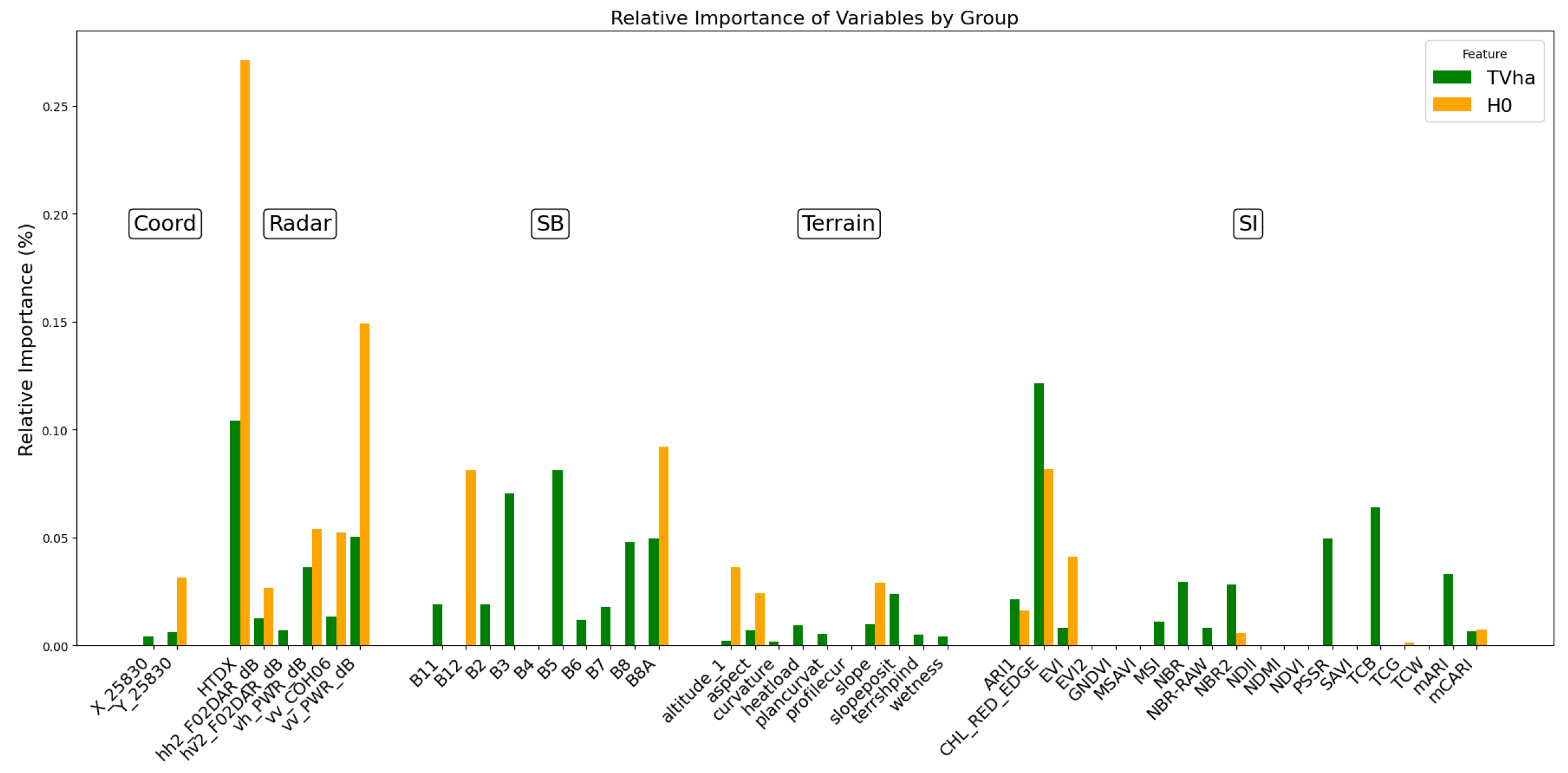
We evaluated a feature reduction system based on Lasso. We analyzed three different feature sets for each model,
and
. We selected the variables on the basis of their importance (
Figure 4. The first group was formed by those variables that, when summed, exceeded 40% of the importance. The second group included those variables whose combined value was more than 75%. Finally, the third group consisted of all variables whose importance was higher than 1%.
The performance metrics for five regression models (kNN, LGBM, MLR, RF, and XGBoost) under three configurations, corresponding to increasing numbers of variables (N Var = 5, 13, 23) are shown in
Table 9. The metrics evaluated include R
2, bias (absolute and percentage), RMSE, and relative RMSE (RMSE (%)). In general, the perfomance of all models improved as the number of variables increased, and only kNN performed better with a medium number of variables. Among the models, XGBoost produced the best results with an R
2 of 0.49, the lowest RMSE (109.07), and a minimal bias percentage of −1.30% when using 23 variables. This result is better than when all features were used. The best-performing model was LGBM, particularly in terms of RMSE and RMSE (%), but it did not surpass XGBoost in overall performance.
The same analysis was conducted for the dominant height (
Table 10), and three configurations with varying numbers of predictors (
N Var = 2, 7, 16) were calculated. As with the total volume, the performance of all models, apart from kNN, consistently improved as the number of predictive variables increased. Among the metrics considered (
, bias, percentage bias, RMSE, and RMSE (%)), LGBM performed best overall, yielding the highest R
2 (0.49) and the lowest RMSE (4.99) and RMSE (%) (24.12%) with 16 predictors. XGBoost and MLR also exhibited a high predictive capacity, with R
2 and error metrics comparable to those of XGBoost, particularly when more predictors were included.
On the other hand, the performance of kNN and RF was intermediate, with slightly higher RMSE and RMSE (%) values than for XGBoost and LGBM. However, the low percentage bias of RF (0.99% with 15 variables) indicates consistent predictions, although this model falls short of XGBoost in terms of .
Overall, XGBoost emerged as the most effective model for this dataset due to its high predictive accuracy and low error rates across all configurations, making it the optimal choice for modeling the target variable.
3.3. Forest Plantation Models
We developed eight forest models for each target variable to examine the influence of the species on the spectral signature and the contribution of work with each species separately. We selected the best models from the previous analysis: LightGBM for and XGBoost for .
Table 11 includes the statistical results for two features,
and
, for three tree species:
Eucalyptus globulus,
Pinus radiata, and
Pinus pinaster, as well as for the whole Forest Plantations group. For the characteristic
, the R
2 values indicate moderate predictive power for all species and forest plantations, with
Pinus pinaster yielding the highest value of 0.51, while
Eucalyptus globulus and
Pinus radiata have similar values close to 0.44. The bias was generally low, with
Pinus radiata showing a bias close to zero (0). The RMSE values were lowest for
Pinus pinaster (4.19). The lowest RMSE (%) corresponded to
Pinus radiata (19%). Compared to previous studies, the inclusion of the TanDEM-X height provides valuable information and improved previous results (R
2 around 0.37 for each species).
For the
feature, the R
2 values were higher for
Pinus pinaster (0.61) and lower for
Pinus radiata (0.35). The negative bias was highest
for Pinus radiata (−2.87), with the predicted values being underestimated, while the positive bias was low (0.44) for
Pinus pinaster, with the predicted values being overestimated. The RMSE values for
show that the model performed worse than
. In terms of relative error,
Eucalyptus globulus yielded the highest RMSE (%) (60%), indicating greater variability in the predictions than for the other species. In previous studies, such as [
61], the R
2 value for this variable was around 0.45, and lower values were obtained in the current study.
In general, these results show that the predictions were better for
Pinus pinaster in both cases. This could be due to the type of stand formed by
Pinus pinaster, in which annual growth is the lowest among the three species, so the variability in radar data acquisition between 2018 and 2019 did not have as great an influence as on
Eucalyptus globulus, which has higher average growth rates. As a result,
Pinus pinaster remained more stable over time, which could explain this better fit for the species. Analysis of the dominant height CAI for each species obtained from the site quality curves of [
64] from Galicia for the study area yielded the following values:
E. globulus: 1.82 m year
−1,
P. radiata: 0.80 m year
−1, and
P. pinaster: 0.55 m year
−1. Therefore, the lack of temporal correlation between field data collection and image acquisition had less influence on the species with the slowest growth rates.
In comparison with the results obtained by [
61], there was a significant improvement for
Pinus pinaster, for which an R
2 value of 0.45 was obtained in the earlier study. Comparing the results of the forest plantations with the individual species showed that the plantations generally tended to yield intermediate results between those obtained for the individual species. In the case of
, the R
2 value for the forest plantations was 0.49, which is higher than for
Pinus radiata but lower than for
Pinus pinaster. For
, the forest plantations yielded an R
2 of 0.49, also between the values for the individual species. Additionally, the bias and RMSE of the plantations tend to be intermediate, providing a more stable prediction than with the species-specific models.
When we compare the results of this study with other similar studies on tree height or forest stock in m³/ha, we find that the results are in line with those obtained by other researchers, such as [
19] (R
2 for E globulus in a total volume of 0.52) and [
39] (R
2 in a total volume of 0.58). However, with similar EO data databases but different field data, the results presented by authors like [
26] (R
2 for E globulus in a total volume of 0.78, RMSE (%) = 23%) or [
24] (R
2 in a total volume of 0.65–0.74) were better than those obtained in this study, emphasizing the influence of these differences in model generation, where the study range, shape, and number of plots play a crucial role in the outcomes. For example, the total volume range in the plots of this study spans from 0.68 to around 700 m³/ha, while that in [
24] ranges from 12 to 253 m³/ha.
It has to be noted also that this study was conducted using ARD data sources, which enables the correponding analysis to be conducted on cloud computing platforms without the need for image processing. While it has been shown that precise topographic corrections affect predictions [
61,
65], the trade-off between improving these corrections and the time and resources spent on this should be assessed.
On the other hand, adopting an approach focused on forest plantations enables the development of more stable models. The size of the training dataset and the increased variability in the data are considered to be the main reasons for the improved stability. By integrating data from different species, greater diversity in spectral and growth characteristics is introduced, which allows the model to better generalize across various conditions. This reduces overfitting to a particular species and results in more consistent predictions. Such an approach could even accommodate mixed plantation plots, although these types of plots were not used in this study.
Final plots with the reference vs. predicted values are shown in
Figure 5 and
Figure 6.
The application of one of the generated models can be seen in
Figure 7. In comparison with the high-resolution image, it is evident how the model-generated information adapts to the study area. However, as stated by [
61], these maps derived from spatially continuous variables should be clipped using accurate land cover classification maps to precisely delineate the area occupied by forest plantations on the ground.
3.4. Limitations and Further Studies
The main limitation of this study is the temporal harmonization of the data. TanDEM-X data are only available in derived products for 2018–2019, highlighting the need for annual mosaics for better forest height prediction. It also has to be remembered that the models are highly dependent on the field reference datasets, as discussed above, and the findings of this study therefore cannot be generalized to other regions.
There are at least three aspects that need further research and may potentially significantly improve the approaches tested in this study. These include the development of models for mixed forest plantations, the utilization of L-band repeat-pass interferometry, and the development of deep learning methodologies. The current study will serve as a good benchmark for the evaluation of improvements that can be achieved by additional datasets and deep learning models. Other future lines of research include the combination of several types of sensors under deep learning techniques [
66] and the analysis of temporal series [
67,
68].
This article is part of a study on prediction using deep learning algorithms and will be used as a comparison between models developed using deep learning and traditional machine learning algorithms.
4. Conclusions
The results of this study indicate that the models that combine optical and imaging radar data acquired by Sentinel-1, ALOS-2 PALSAR-2, and TanDEM-X satellites generally perform best, in terms of R2, bias, and RMSE, outperforming models that use only one type of sensor data. Terrain variables make little contribution to improving the models. The addition of climate variables does not seem to provide significant improvements in prediction accuracy, although it does help refine the predictions in some cases. Models enabling wall-to-wall mapping tend to perform slightly less well than the best optical + radar combination models, but yield acceptable results for operational purposes.
The best machine learning (ML) algorithms for each forest variable were LightGBM for total height and XGBoost for , specifically for the study area and the forest stands analyzed, namely Pinus pinaster, Pinus radiata, and Eucalyptus globulus. The variable reduction suggests that only the kNN method benefited from optimized feature reduction.
The models developed for forest plantations were more stable than generic models, although the best results obtained for Pinus pinaster were probably due to the stability of the stands over time. However, generic plantation models can be useful for predicting volume in mixed plantations of these species in the study area.
The temporal harmonization of the data is a limitation, as TanDEM-X data are only available in derived products for 2018–2019, highlighting the need for annual mosaics for better forest height prediction. Future research should focus on mixed forest plantations, L-band repeat-pass interferometry, and deep learning methodologies, with this article serving as a comparison between deep learning and traditional machine learning models.


 ,
, 
