
Using Unoccupied Aerial Systems (UAS) and Structure-from-Motion (SfM) to Measure Forest Canopy Cover and Individual Tree Height Metrics in Northern California Forests


Abstract
1. Introduction
2. Materials and Methods
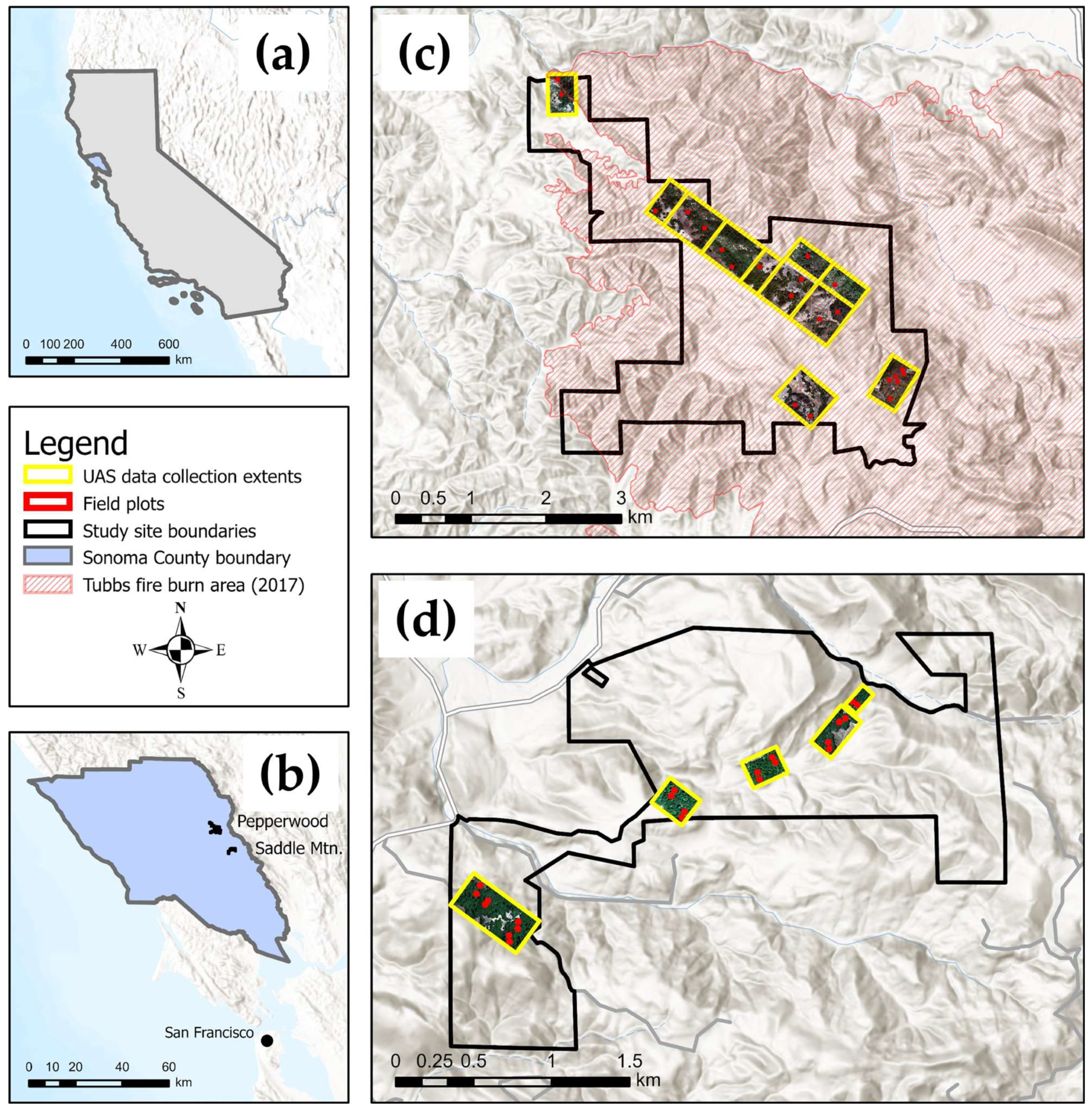
2.1. Study Sites
- Twenty-two 20 m × 20 m long-term plots at Pepperwood Preserve, stratified based on topographic gradients, ecological heterogeneity, and post-fire burn severity;
- Twenty-two 11.3 m radius plots at Saddle Mountain, selected to represent varying forest structures and dominant species across the preserve’s topographic gradient.
2.2. Ground-Based Field Data Collection
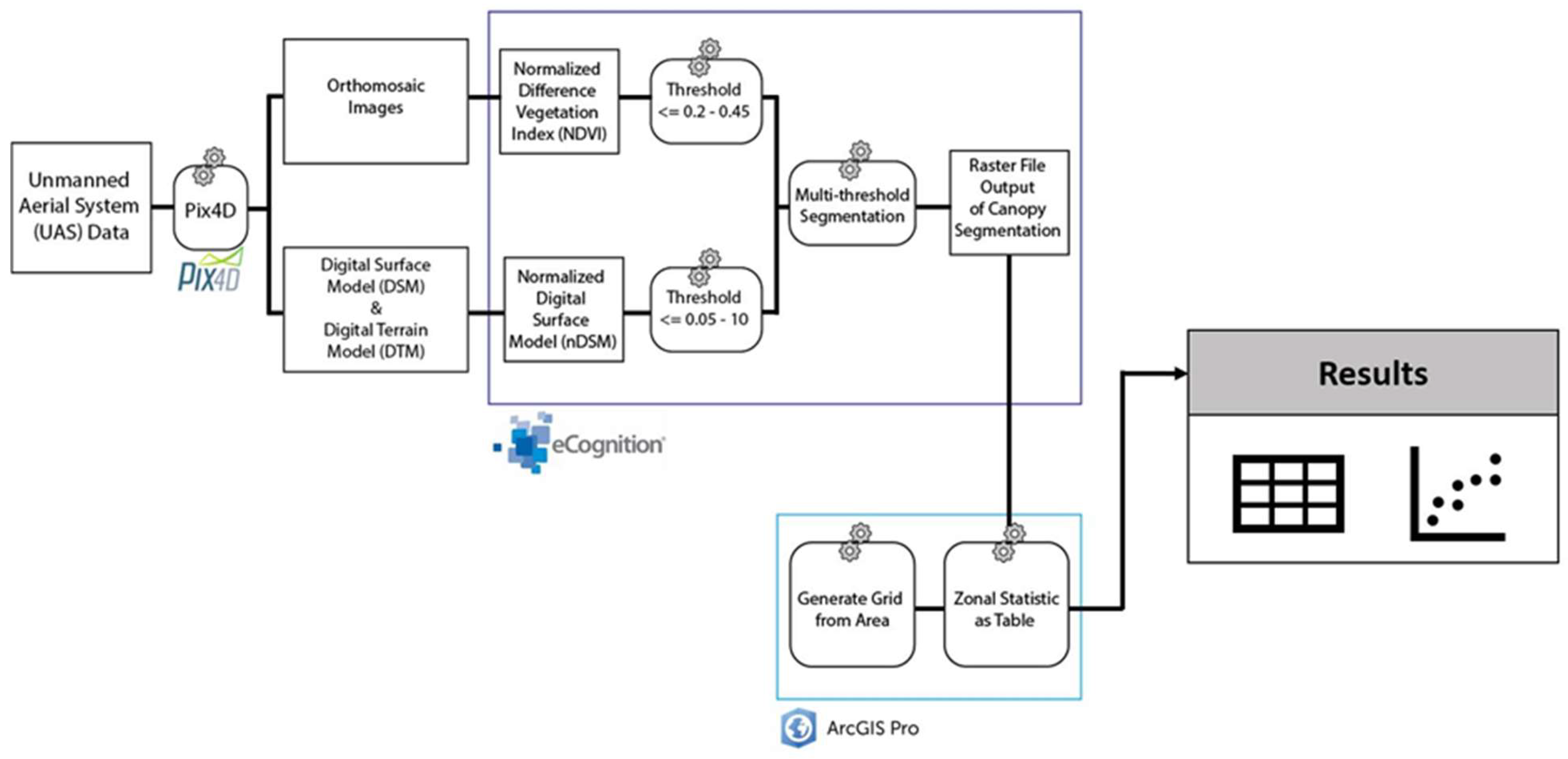
2.3. Unoccupied Aerial System (UAS) Structure from Motion (SfM) Multispectral Data Collection and Processing
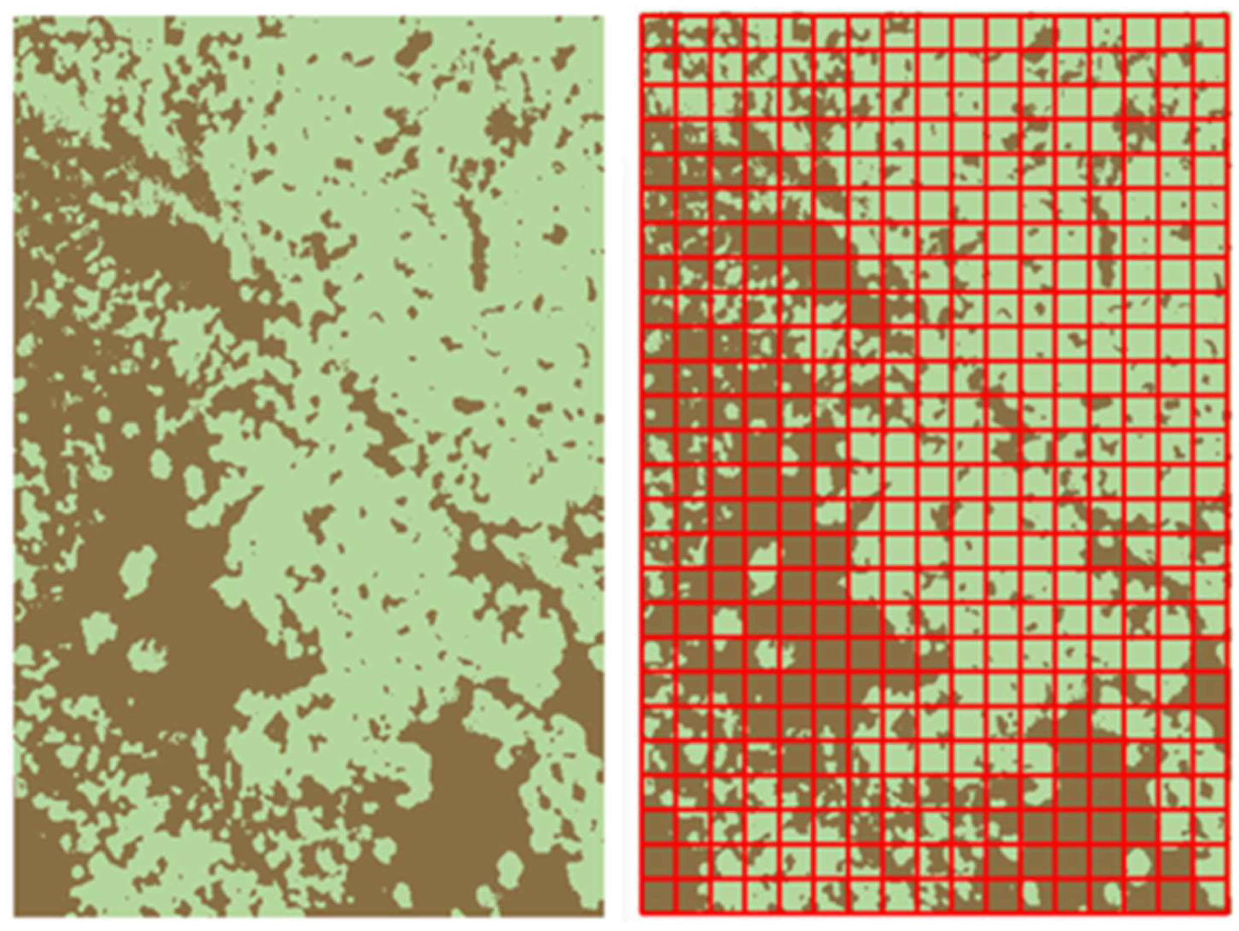
2.4. UAS-Derived Canopy Cover Estimates
2.5. Individual Tree Detection (ITD)
2.6. Accuracy Assessment of Tree Detections
- Density class one: Plots with 3, 5, 7, and 8 trees (7 plots)
- Density class two: Plots with 9, 12, 13, and 14 trees (7 plots)
- Density class three: Plots with 16, 17, 18, 19, and 20 trees (12 plots)
- Density class four: Plots with 21, 23, 24, 26, 29, 30, and 31 trees (10 plots)
- Density class five: Plots with 32, 34, 37, 38, 39, 44, and 58 trees (8 plots)
2.7. Derivation of Individual Tree Metrics
3. Results
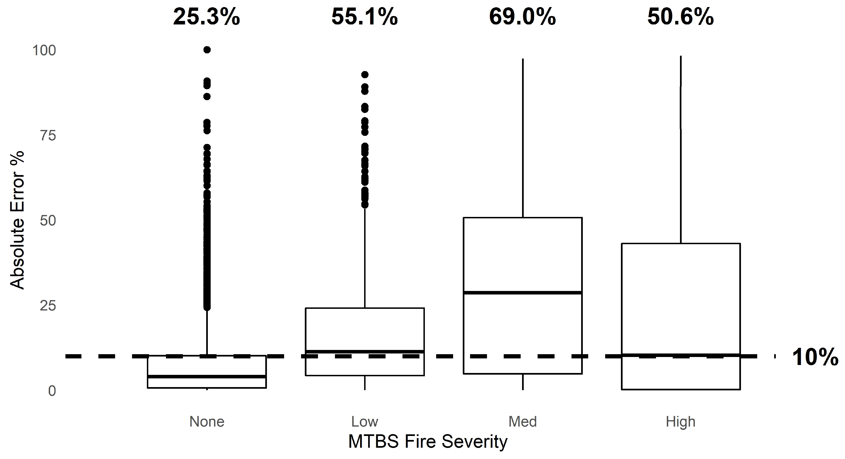
3.1. Canopy Cover
3.2. Individual Tree Detection
3.3. Individual Tree Metrics
- Conifer trees had a more significant linear relationship with field measurements (r2 = 0.69, p < 0.0001) and had a higher RMSE (6.17 m; Figure 7C)
4. Discussion
4.1. Feasibility of UAS-SfM for Forest Structure Estimation
4.2. Canopy Cover Estimations
4.3. Individual Tree Detection and Segmentation
4.4. Tree Height and Canopy Base Height Estimations
4.5. Future Recommendations
5. Conclusions
Supplementary Materials
Author Contributions
Funding
Data Availability Statement
Acknowledgments
Conflicts of Interest
References
- Gaman, T.; Firman, J. Oaks 2040: The Status and Future of Oaks in California; California Oak Foundation: Oakland, CA, USA, 2006; p. 14. [Google Scholar]
- Holmes, K.A.; Veblen, K.E.; Young, T.P.; Berry, A.M. California Oaks and Fire: A Review and Case Study. In Proceedings of the Sixth California Oak Symposium: Today’s Challenges, Tomorrow’s Opportunities, Rohnert Park, CA, USA, 9–12 October 2006. [Google Scholar]
- Stuart, J.D.; Stephens, S.L.; Agee, J.K. North Coast Bioregion. In Fire in California’s Ecosystems; Sugihara, N.G., Van Wagtendonk, J.W., Shaffer, K.E., Fites-Kaufman, J., Thode, A.E., Eds.; University of California Press: Berkeley, CA, USA, 2006; pp. 147–169. ISBN 978-0-520-24605-8. [Google Scholar]
- Bernhardt, E.A.; Swiecki, T.J. Restoring Oak Woodlands in California: Theory and Practice. Available online: http://phytosphere.com/restoringoakwoodlands/oakrestoration.htm (accessed on 22 May 2022).
- Forest Management Task Force. California’s Wildfire and Forest Resilience Action Plan; State of California: Sacramento, CA, USA, 2021. [Google Scholar]
- Miraki, M.; Sohrabi, H.; Fatehi, P.; Kneubuehler, M. Individual Tree Crown Delineation from High-Resolution UAV Images in Broadleaf Forest. Ecol. Inform. 2021, 61, 101207. [Google Scholar] [CrossRef]
- Shin, P.; Sankey, T.; Moore, M.; Thode, A. Evaluating Unmanned Aerial Vehicle Images for Estimating Forest Canopy Fuels in a Ponderosa Pine Stand. Remote Sens. 2018, 10, 1266. [Google Scholar] [CrossRef]
- Ke, Y.; Quackenbush, L.J. A Review of Methods for Automatic Individual Tree-Crown Detection and Delineation from Passive Remote Sensing. Int. J. Remote Sens. 2011, 32, 4725–4747. [Google Scholar] [CrossRef]
- Aubry-Kientz, M.; Dutrieux, R.; Ferraz, A.; Saatchi, S.; Hamraz, H.; Williams, J.; Coomes, D.; Piboule, A.; Vincent, G. A Comparative Assessment of the Performance of Individual Tree Crowns Delineation Algorithms from ALS Data in Tropical Forests. Remote Sens. 2019, 11, 1086. [Google Scholar] [CrossRef]
- Weinstein, B.G.; Marconi, S.; Bohlman, S.A.; Zare, A.; White, E.P. Cross-Site Learning in Deep Learning RGB Tree Crown Detection. Ecol. Inform. 2020, 56, 101061. [Google Scholar] [CrossRef]
- Wallace, L.; Lucieer, A.; Malenovský, Z.; Turner, D.; Vopěnka, P. Assessment of Forest Structure Using Two UAV Techniques: A Comparison of Airborne Laser Scanning and Structure from Motion (SfM) Point Clouds. Forests 2016, 7, 62. [Google Scholar] [CrossRef]
- Reilly, S.; Clark, M.L.; Loechler, L.; Spillane, J.; Kozanitas, M.; Krause, P.; Ackerly, D.; Bentley, L.P.; Menor, I.O. Unoccupied Aerial System (UAS) Structure-from-Motion Canopy Fuel Parameters: Multisite Area-Based Modelling across Forests in California, USA. Remote Sens. Environ. 2024, 312, 114310. [Google Scholar] [CrossRef]
- Li, W.; Guo, Q.; Jakubowski, M.K.; Kelly, M. A New Method for Segmenting Individual Trees from the Lidar Point Cloud. Photogramm. Eng. Remote Sens. 2012, 78, 75–84. [Google Scholar] [CrossRef]
- Andersen, H.-E.; McGaughey, R.J.; Reutebuch, S.E. Estimating Forest Canopy Fuel Parameters Using LIDAR Data. Remote Sens. Environ. 2005, 94, 441–449. [Google Scholar] [CrossRef]
- Erdody, T.L.; Moskal, L.M. Fusion of LiDAR and Imagery for Estimating Forest Canopy Fuels. Remote Sens. Environ. 2010, 114, 725–737. [Google Scholar] [CrossRef]
- Jaskierniak, D.; Lucieer, A.; Kuczera, G.; Turner, D.; Lane, P.N.J.; Benyon, R.G.; Haydon, S. Individual Tree Detection and Crown Delineation from Unmanned Aircraft System (UAS) LiDAR in Structurally Complex Mixed Species Eucalypt Forests. ISPRS J. Photogramm. Remote Sens. 2021, 171, 171–187. [Google Scholar] [CrossRef]
- Panagiotidis, D.; Abdollahnejad, A.; Surový, P.; Chiteculo, V. Determining Tree Height and Crown Diameter from High-Resolution UAV Imagery. Int. J. Remote Sens. 2017, 38, 2392–2410. [Google Scholar] [CrossRef]
- Shin, P. Unmanned Aerial Vehicles for Estimating Forest Canopy Fuels in Ponderosa Pine Forest. Master’s Thesis, Northern Arizona University, Flagstaff, AZ, USA, 2018. [Google Scholar]
- Westoby, M.J.; Brasington, J.; Glasser, N.F.; Hambrey, M.J.; Reynolds, J.M. ‘Structure-from-Motion’ Photogrammetry: A Low-Cost, Effective Tool for Geoscience Applications. Geomorphology 2012, 179, 300–314. [Google Scholar] [CrossRef]
- Dandois, J.P.; Ellis, E.C. High Spatial Resolution Three-Dimensional Mapping of Vegetation Spectral Dynamics Using Computer Vision. Remote Sens. Environ. 2013, 136, 259–276. [Google Scholar] [CrossRef]
- Morgenroth, J.; Gomez, C. Assessment of Tree Structure Using a 3D Image Analysis Technique—A Proof of Concept. Urban For. Urban Green. 2014, 13, 198–203. [Google Scholar] [CrossRef]
- Frankhauser, P.; Tannier, C.; Vuidel, G.; Houot, H. An Integrated Multifractal Modelling to Urban and Regional Planning. Comput. Environ. Urban Syst. 2018, 67, 132–146. [Google Scholar] [CrossRef]
- Liu, L.; Lim, S.; Shen, X.; Yebra, M. A Hybrid Method for Segmenting Individual Trees from Airborne Lidar Data. Comput. Electron. Agric. 2019, 163, 104871. [Google Scholar] [CrossRef]
- Lim, Y.S.; La, P.H.; Park, J.S.; Lee, M.H.; Pyeon, M.W.; Kim, J.-I. Calculation of Tree Height and Canopy Crown from Drone Images Using Segmentation. J. Korean Soc. Surv. Geod. Photogramm. Cartogr. 2015, 33, 605–614. [Google Scholar] [CrossRef]
- Forbes, B.; Reilly, S.; Clark, M.; Ferrell, R.; Kelly, A.; Krause, P.; Matley, C.; O’Neil, M.; Villasenor, M.; Disney, M.; et al. Comparing Remote Sensing and Field-Based Approaches to Estimate Ladder Fuels and Predict Wildfire Burn Severity. Front. For. Glob. Change 2022, 5, 818713. [Google Scholar] [CrossRef]
- Bowers, C.L. The Diablo Winds of Northern California: Climatology and Numerical Simulations. Master’s Thesis, San Jose State University, San Jose, CA, USA, 2018. [Google Scholar]
- CAL FIRE Fire Hazard Severity Zones (FHSZ). Available online: https://osfm.fire.ca.gov/divisions/community-wildfire-preparedness-and-mitigation/wildfire-preparedness/fire-hazard-severity-zones/ (accessed on 22 May 2022).
- Gillogly, M.; Dodge, C.; Halbur, M.; Micheli, L.; McKay, C.; Heller, N.; Benson, B. Adaptive Management Plan for Pepperwood Preserve; Dwight Center for Conservation Science: Pepperwood, Santa Rosa, CA, 2017. [Google Scholar]
- Ag + Open Space. Saddle Mountain Open Space Preserve Management Plan; Ag + Open Space: Santa Rosa, CA, USA, 2019. [Google Scholar]
- Lemmon, P.E. A Spherical Densiometer for Estimating Forest Overstory Density. For. Sci. 1956, 2, 314–320. [Google Scholar]
- Lemmon, P.E. A New Instrument for Measuring Forest Overstory Density. J. For. 1957, 55, 667–668. [Google Scholar]
- Reilly, S.; Clark, M.L.; Bentley, L.P.; Matley, C.; Piazza, E.; Oliveras Menor, I. The Potential of Multispectral Imagery and 3D Point Clouds from Unoccupied Aerial Systems (UAS) for Monitoring Forest Structure and the Impacts of Wildfire in Mediterranean-Climate Forests. Remote Sens. 2021, 13, 3810. [Google Scholar] [CrossRef]
- Trimble Support Tree Crown Delineation. Available online: https://support.ecognition.com/hc/en-us/articles/360016224679-Tree-Crown-Delineation (accessed on 11 March 2022).
- Eidenshink, J.; Schwind, B.; Brewer, K.; Zhu, Z.-L.; Quayle, B.; Howard, S. A Project for Monitoring Trends in Burn Severity. Fire Ecol. 2007, 3, 3–21. [Google Scholar] [CrossRef]
- Picotte, J.J.; Bhattarai, K.; Howard, D.; Lecker, J.; Epting, J.; Quayle, B.; Benson, N.; Nelson, K. Changes to the Monitoring Trends in Burn Severity Program Mapping Production Procedures and Data Products. Fire Ecol. 2020, 16, 16. [Google Scholar] [CrossRef]
- Roussel, J.-R.; Auty, D.; Coops, N.C.; Tompalski, P.; Goodbody, T.R.H.; Meador, A.S.; Bourdon, J.-F.; de Boissieu, F.; Achim, A. lidR: An R Package for Analysis of Airborne Laser Scanning (ALS) Data. Remote Sens. Environ. 2020, 251, 112061. [Google Scholar] [CrossRef]
- Zhang, C.; Zhou, J.; Wang, H.; Tan, T.; Cui, M.; Huang, Z.; Wang, P.; Zhang, L. Multi-Species Individual Tree Segmentation and Identification Based on Improved Mask R-CNN and UAV Imagery in Mixed Forests. Remote Sens. 2022, 14, 874. [Google Scholar] [CrossRef]
- Schiefer, F.; Kattenborn, T.; Frick, A.; Frey, J.; Schall, P.; Koch, B.; Schmidtlein, S. Mapping Forest Tree Species in High Resolution UAV-Based RGB-Imagery by Means of Convolutional Neural Networks. ISPRS J. Photogramm. Remote Sens. 2020, 170, 205–215. [Google Scholar] [CrossRef]
- Qin, H.; Zhou, W.; Yao, Y.; Wang, W. Individual Tree Segmentation and Tree Species Classification in Subtropical Broadleaf Forests Using UAV-Based LiDAR, Hyperspectral, and Ultrahigh-Resolution RGB Data. Remote Sens. Environ. 2022, 280, 113143. [Google Scholar] [CrossRef]
- Windrim, L.; Bryson, M. Detection, Segmentation, and Model Fitting of Individual Tree Stems from Airborne Laser Scanning of Forests Using Deep Learning. Remote Sens. 2020, 12, 1469. [Google Scholar] [CrossRef]
- Krause, P.; Forbes, B.; Barajas-Ritchie, A.; Clark, M.; Disney, M.; Wilkes, P.; Bentley, L.P. Using Terrestrial Laser Scanning to Evaluate Non-Destructive Aboveground Biomass Allometries in Diverse Northern California Forests. Front. Remote Sens. 2023, 4, 1132208. [Google Scholar]
- Jennings, S. Assessing Forest Canopies and Understorey Illumination: Canopy Closure, Canopy Cover and Other Measures. Forestry 1999, 72, 59–74. [Google Scholar] [CrossRef]
- Englund, S.R.; O’Brien, J.J.; Clark, D.B. Evaluation of Digital and Film Hemispherical Photography and Spherical Densiometry for Measuring Forest Light Environments. Can. J. For. Res. 2000, 30, 1999–2005. [Google Scholar] [CrossRef]
- McIntosh, A.C.S.; Gray, A.N.; Garman, S.L. Estimating Canopy Cover from Standard Forest Inventory Measurements in Western Oregon. For. Sci. 2012, 58, 154–167. [Google Scholar] [CrossRef]
- Paletto, A.; Tosi, V. Forest Canopy Cover and Canopy Closure: Comparison of Assessment Techniques. Eur. J. For. Res. 2009, 128, 265–272. [Google Scholar] [CrossRef]
- Ramalho de Oliveira, L.F.; Lassiter, H.A.; Wilkinson, B.; Whitley, T.; Ifju, P.; Logan, S.R.; Peter, G.F.; Vogel, J.G.; Martin, T.A. Moving to Automated Tree Inventory: Comparison of UAS-Derived Lidar and Photogrammetric Data with Manual Ground Estimates. Remote Sens. 2020, 13, 72. [Google Scholar] [CrossRef]
- Zaforemska, A.; Xiao, W.; Gaulton, R. Individual Tree Detection from UAV LiDAR Data in a Mixed Species Woodland. Int. Arch. Photogramm. Remote Sens. Spat. Inf. Sci. 2019, 42, 657–663. [Google Scholar] [CrossRef]
- Reeves, M.C.; Ryan, K.C.; Rollins, M.G.; Thompson, T.G. Spatial Fuel Data Products of the LANDFIRE Project. Int. J. Wildland Fire 2009, 18, 250. [Google Scholar] [CrossRef]


| A. | Density Class One (3–8 Trees/Plot) | |||||||||
| Plots: 1, 2, 1303, 1304, 1309, 1349, 1852 | ||||||||||
| Total Trees: 41 | ||||||||||
| DT Value | Search Radius | Minimum Height | NDVI Threshold | Detected Trees (%) | Commission Error (%) | Omitted Trees (%) | r | p | F-1 | |
| 1 | 1 | 1 | 0.04 | 93 | 666 | 7 | 0.93 | 0.12 | 0.22 | |
| 1 | 3 | 2 | 0.04 | 78 | 278 | 22 | 0.78 | 0.22 | 0.34 | |
| 5 | 1 | 1 | 0.04 | 73 | 27 | 27 | 0.73 | 0.73 | 0.73 | |
| 1 | 3 | 3 | 0.2 | 78 | 268 | 22 | 0.78 | 0.23 | 0.35 | |
| 2 | 3 | 3 | 0.2 | 61 | 156 | 39 | 0.61 | 0.28 | 0.38 | |
| B. | Density Class Two (9–14 Trees/Plot) | |||||||||
| Plots: 12, 1306, 1307, 1310, 1319, 1340, 1851 | ||||||||||
| Total Trees: 79 | ||||||||||
| DT Value | Search Radius | Minimum Height | NDVI Threshold | Detected Trees (%) | Commission Error (%) | Omitted Trees (%) | r | p | F-1 | |
| 1 | 1 | 1 | 0.04 | 91 | 286 | 9 | 0.91 | 0.24 | 0.38 | |
| 1 | 3 | 2 | 0.04 | 82 | 96 | 18 | 0.82 | 0.46 | 0.59 | |
| 5 | 1 | 1 | 0.04 | 37 | 26 | 172 | 0.18 | 0.59 | 0.27 | |
| 1 | 3 | 3 | 0.2 | 81 | 94 | 19 | 0.81 | 0.46 | 0.59 | |
| 2 | 3 | 3 | 0.2 | 70 | 46 | 30 | 0.70 | 0.60 | 0.65 | |
| C. | Density Class Three (16–20 Trees/Plot) | |||||||||
| Plots: 11, 16, 18, 19, 1301, 1325, 1329, 1335, 1336, 1337, 1342, 1854 | ||||||||||
| Total Trees: 215 | ||||||||||
| DT Value | Search Radius | Minimum Height | NDVI Threshold | Detected Trees (%) | Commission Error (%) | Omitted Trees (%) | r | p | F-1 | |
| 1 | 1 | 1 | 0.04 | 89 | 172 | 11 | 0.89 | 0.34 | 0.49 | |
| 1 | 3 | 2 | 0.04 | 76 | 44 | 24 | 0.76 | 0.64 | 0.69 | |
| 5 | 1 | 1 | 0.04 | 34 | 8 | 66 | 0.34 | 0.81 | 0.48 | |
| 1 | 3 | 3 | 0.2 | 73 | 41 | 27 | 0.73 | 0.64 | 0.68 | |
| 2 | 3 | 3 | 0.2 | 56 | 21 | 44 | 0.56 | 0.72 | 0.63 | |
| D. | Density Class Four (21–31 Trees/Plot) | |||||||||
| Plots: 3, 5, 15, 17, 20, 24, 25, 26, 1315, 1853 | ||||||||||
| Total Trees: 270 | ||||||||||
| DT Value | Search Radius | Minimum Height | NDVI Threshold | Detected Trees (%) | Commission Error (%) | Omitted Trees (%) | r | p | F-1 | |
| 1 | 1 | 1 | 0.04 | 81 | 99 | 19 | 0.81 | 0.45 | 0.58 | |
| 1 | 3 | 2 | 0.04 | 61 | 17 | 39 | 0.61 | 0.78 | 0.68 | |
| 5 | 1 | 1 | 0.04 | 21 | 0 | 79 | 0.21 | 1.00 | 0.35 | |
| 1 | 3 | 3 | 0.2 | 60 | 12 | 40 | 0.60 | 0.83 | 0.70 | |
| 2 | 3 | 3 | 0.2 | 45 | 6 | 55 | 0.45 | 0.89 | 0.60 | |
| E. | Density Class Five (32–58 Trees/Plot) | |||||||||
| Plots: 4, 6, 7, 8, 13, 14, 23, 1332 | ||||||||||
| Total Trees: 299 | ||||||||||
| DT Value | Search Radius | Minimum Height | NDVI Threshold | Detected Trees (%) | Commission Error (%) | Omitted Trees (%) | r | p | F-1 | |
| 1 | 1 | 1 | 0.04 | 72 | 49 | 28 | 0.72 | 0.59 | 0.65 | |
| 1 | 3 | 2 | 0.04 | 39 | 17 | 61 | 0.39 | 0.70 | 0.50 | |
| 5 | 1 | 1 | 0.04 | 13 | 1 | 87 | 0.13 | 0.95 | 0.22 | |
| 1 | 3 | 3 | 0.2 | 46 | 16 | 54 | 0.46 | 0.74 | 0.57 | |
| 2 | 3 | 3 | 0.2 | 30 | 7 | 70 | 0.30 | 0.82 | 0.44 | |
Disclaimer/Publisher’s Note: The statements, opinions and data contained in all publications are solely those of the individual author(s) and contributor(s) and not of MDPI and/or the editor(s). MDPI and/or the editor(s) disclaim responsibility for any injury to people or property resulting from any ideas, methods, instructions or products referred to in the content. |
© 2025 by the authors. Licensee MDPI, Basel, Switzerland. This article is an open access article distributed under the terms and conditions of the Creative Commons Attribution (CC BY) license (https://creativecommons.org/licenses/by/4.0/).
Share and Cite
Kelly, A.; Blesius, L.; Davis, J.D.; Bentley, L.P. Using Unoccupied Aerial Systems (UAS) and Structure-from-Motion (SfM) to Measure Forest Canopy Cover and Individual Tree Height Metrics in Northern California Forests. Forests 2025, 16, 564. https://doi.org/10.3390/f16040564
Kelly A, Blesius L, Davis JD, Bentley LP. Using Unoccupied Aerial Systems (UAS) and Structure-from-Motion (SfM) to Measure Forest Canopy Cover and Individual Tree Height Metrics in Northern California Forests. Forests. 2025; 16(4):564. https://doi.org/10.3390/f16040564
Chicago/Turabian StyleKelly, Allison, Leonhard Blesius, Jerry D. Davis, and Lisa Patrick Bentley. 2025. "Using Unoccupied Aerial Systems (UAS) and Structure-from-Motion (SfM) to Measure Forest Canopy Cover and Individual Tree Height Metrics in Northern California Forests" Forests 16, no. 4: 564. https://doi.org/10.3390/f16040564
APA StyleKelly, A., Blesius, L., Davis, J. D., & Bentley, L. P. (2025). Using Unoccupied Aerial Systems (UAS) and Structure-from-Motion (SfM) to Measure Forest Canopy Cover and Individual Tree Height Metrics in Northern California Forests. Forests, 16(4), 564. https://doi.org/10.3390/f16040564