Article

Analysis of the Application of Machine Learning Algorithms Based on Sentinel-1/2 and Landsat 8 OLI Data in Estimating Above-Ground Biomass of Subtropical Forests

1
College of Forestry, Southwest Forestry University, Kunming 650224, China
2
School of Geosciences, University of Edinburgh, Edinburgh EH8 9XP, UK
3
Royal Botanic Garden Edinburgh, Edinburgh EH3 5LR, UK
4
College of Soil and Water Conservation, Southwest Forestry University, Kunming 650224, China
*
Author to whom correspondence should be addressed.
Forests 2025, 16(4), 559; https://doi.org/10.3390/f16040559
Submission received: 14 February 2025 / Revised: 12 March 2025 / Accepted: 21 March 2025 / Published: 23 March 2025
(This article belongs to the Section Forest Inventory, Modeling and Remote Sensing)

Abstract

:
Accurate monitoring of aboveground biomass (AGB) in subtropical forests plays an important role in maintaining biodiversity and the balance of forest ecosystems. It is of high importance to explore how machine learning models can improve the ability and accuracy of AGB estimation of different types of subtropical forests under the conditions of active and passive open-source remote sensing (RS) data. In this study, the subtropical forests in the Pu’er region of Yunnan Province were used as the research object, and backscattering coefficients, mean reflectance, and textural features from Sentinel-1, Sentinel-2, and Landsat 8 OLI open-source RS data were used as the data source. We classified the subtropical forests into three basic forest types: broadleaf forest, coniferous forest, and mixed forest. Based on filtering and analyzing RS features, we performed forest AGB inversion using Random Forest (RF), Support Vector Regression (SVR), and eXtreme Gradient Boosting (XGBoost). The results show that: (1) VH-related texture features in Sentinel-1, and red-edge band features, IR band features, and texture features in Sentinel-2 and Landsat 8 OLI are sensitive to changes in forest AGB. (2) Among the three nonparametric methods, the XGBoost algorithm had the highest estimation accuracy with an MAE of 10.05 t/ha and RMSE of 12.43 t/ha in coniferous forests; the second estimation accuracy in mixed forests with an MAE of 20.18 t/ha and RMSE of 25.33 t/ha; and the estimation accuracy in broad-leaved forests with an MAE of 25.22 t/ha and RMSE of 32.32 t/ha. (3) The accuracy of estimating forest AGB by combining multiple RS data is higher than the estimation results using a single RS data. We found that the VH features of SAR data contribute more to the inversion of high-precision forest AGB; the XGBoost model has the strongest robustness and the highest accuracy in the AGB inversion of subtropical forests using multisource RS data. (4) The spatial autocorrelation of the samples themselves also needs to be taken into account when modeling forest AGB estimates.

1. Introduction

Forests are one of the important ecosystems on earth and play an irreplaceable role in the global carbon cycle and climate regulation. Above-ground biomass (AGB) is one of the most important indicators for assessing the productivity, carbon sequestration capacity, and ecological benefits of forests, and accurate and rapid estimation of forest AGB is of great significance in assessing the functions of forests. Compared with the traditional forest AGB estimation methods, the estimation of forest AGB using remote sensing (RS) technology has the advantages of wide range, short revisit period, and long time series [1]. Multispectral, Synthetic Aperture Radar (SAR), and Light Detection and Ranging (LiDAR) data have been used for high-precision forest AGB estimation studies [2,3,4,5]. LiDAR data can accurately obtain 3D structural information of forests, but there are drawbacks such as the high cost of airborne LiDAR data acquisition and small spatial and temporal coverage, which limit its application in forest AGB estimation [6]. Multispectral RS data can continuously acquire forest canopy features, as well as spectral and texture features that are important for forest AGB estimation, and have the advantages of easy access and wide coverage, but multi-spectral data can only acquire the horizontal structure of the forest canopy, and cannot acquire the more complex vertical structure of the forest [7]. SAR data has a certain penetration capacity, so the polarization of SAR data reflects the scattering information of the forest structure. It offers advantages such as being unaffected by cloudy or foggy weather, but the estimates are highly influenced by factors like forest type and topography [8]. Therefore, combining multispectral and SAR data for forest AGB inversion has become a research hotspot, and the open-source Landsat series and Sentinel-1/2 satellite data have the advantage of ease of access, which provides a convenient condition for forest AGB inversion using SAR and multispectral data.
Combining open-source multispectral and SAR data for forest AGB inversion can take advantage of the complementarity of different RS data sources in expressing the information of the structure of forests and then improve the accuracy of forest AGB RS inversion. Li et al. [9] combined Sentinel-1 and Landsat 8 OLI data to invert the forest AGB in Hunan Province, and the results showed that the inversion effect of the combined data was better than that of the single RS data. Zhang et al. [10] used GF1, GF3, and Landsat 8 OLI data for the inversion of forest AGB, and the results showed that synergistic SAR and multispectral data were the best for the inversion. Ding et al. [11] used Landsat 8 OLI, ALOS PALSAR-2, and Sentienl-1 data for forest AGB inversion, and the results showed that the combination of synergistic SAR and multispectral data with machine learning algorithms can accurately and quickly invert large-scale forest AGB. The inversion accuracy of the forest AGB, in addition to being mainly affected by the data source, is also strongly influenced by the construction of different inversion models.
Inversion models for forest AGB are usually categorized into parametric and nonparametric models. Parametric models are simple in structure and interpretable but are unable to characterize the complex nonlinear relationship between forest AGB and remotely sensed features [12]. Nonparametric models have higher inversion accuracy and robustness compared to parametric models, but the inversion results are easily affected by the RS data sources and the extracted RS features [13,14,15,16]. Among the nonparametric models, the commonly used inversion models are Random Forest (RF), K-nearest neighbors (KNN), Artificial Neural Networks (ANN), Support Vector Regression (SVR), Gradient Boosting Decision Trees (GBDT), eXtreme Gradient Boosting Trees (XGBoost), and other models. Zhang et al. [17] estimated forest AGB using KNN, RF, SVR, and deep learning models based on LiDAR data with Landsat 8 OLI data. The results showed that the deep learning model gave the best estimation with R2 = 0.935, RMSE = 15.67 Mg/ha, RMSEr = 11.407%. Awad [18] conducted a qualitative analysis of forest carbon sink estimation using a novel convolutional neural network (FlexibleNet) based on Sentinel-2 data. The results show that FlexibleNet is better compared to four popular convolutional neural networks, ResNet-50, Xception, MobileNetV3-Large, and EfficientNet. Zadbagher et al. [19] forest AGB estimation of peat swamp forests in the humid tropics of Badas based on LiDAR and InSAR data using RF, ANN, and SVM. The results show that SVM has the best estimation, with R2 = 0.71, RMSE = 83.65 Mgha−1, and MAE = 74.73 Mgha−1 for forest AGB. Taken together, the use of deep learning is more effective in the estimation of forest AGB. However, when the number of samples is small, the training effect of the deep learning model cannot be guaranteed, resulting in a lower estimation effect than ordinary machine learning models. In machine learning models, the representative RF model has a good tolerance to outliers and noise, fast training speed, strong robustness, and easily adjustable parameters [20]. However, when the number of decision trees becomes too large, the model consumes high computational resources. SVR excels in handling small samples and high-dimensional problems, with strong generalization ability [6]. However, it is highly sensitive to hyperparameter selection and struggles to guarantee finding the global optimal solution. XGBoost processes faster than traditional gradient-boosting decision trees and adds a regularization term to the loss function to prevent overfitting [21,22]. However, selecting its hyperparameters is more complex and requires higher computational resources. Comparative analysis of nonparametric models with strong model robustness and high inversion accuracy is the current difficulty and hotspot of forest AGB research using RS data.
The subtropical forest of Pu’er City, Yunnan Province, is one of the areas with the largest area of preserved subtropical evergreen broad-leaved forests in China and is a typical representative of subtropical forest ecosystems. Pu’er has an independent and complete flora, which is a typical subtropical-to-tropical transition region in China, and the diversity and uniqueness of its forest types make it a key protection area for China’s primary forest ecosystems [23]. In addition, Pu’er plays an important role in the timber economy of Yunnan and the country as a major source of timber supply and forest products in China [24]. Therefore, it is ecologically and economically important to make full use of the advantages of open-source multi-source RS data to mine the RS features of forest horizontal and vertical structures and then improve the inversion accuracy of forest AGB for accurate monitoring of regional forest AGB in Pu’er City. In this study, we took Simao District of Pu’er City as the study area, and used three open-source RS data, Sentinel-1, Sentinel-2, and Landsat 8 OLI as the data source, to construct three representative machine-learning models, RF, SVR, and XGBoost, for the inversion and detailed analysis of forest AGB. In order to address the following related issues: (1) explore the extent to which relevant RS features, under different RS data combination methods, affect the AGB accuracy of forests of various forest types in the typical subtropics; (2) the suitability and robustness of three representative machine learning models for optimization in subtropical forest AGB inversion. The related research results can provide decision-making for regional forest parameter monitoring and management in Pu’er City, Yunnan Province.

2. Materials and Methods

2.1. Study Area

The study area is located in the southern part of Yunnan Province, in the middle and lower reaches of the Lancang River, in the Pu’er Simao District (22°27′ to 23°06′ N, 100°19′ to 101°27′ E; Figure 1). Simao District, with an altitude of 578 m to 2155 m, is located in the southern part of the Wuliang Mountains of the Hengduan Mountains, with a high topography in the northwest, a low topography in the southeast, and an uplift in the central part of the district. The climate belongs to the southern subtropical monsoon climate of the low latitude plateau, characterized by low latitude, high temperature, and rainy and humid weather. The average temperature is 18.9 °C, and the average precipitation over the years is 1487.5 mm. The forest coverage rate of the whole region is 72.64% [25], and the forest types are mainly tropical monsoon rainforest, broad-leaved forest, and coniferous forest, etc. The main tree species are: Simao pine (Pinus kesiya var. langbianensis (A. Chev.) Gaussen ex Bui), Castanopsis (Castanopsis fargesii Franch.), Quercus (Quercus × leana Nutt.), and Schima superba (Schima superba Gardner and Champ.).

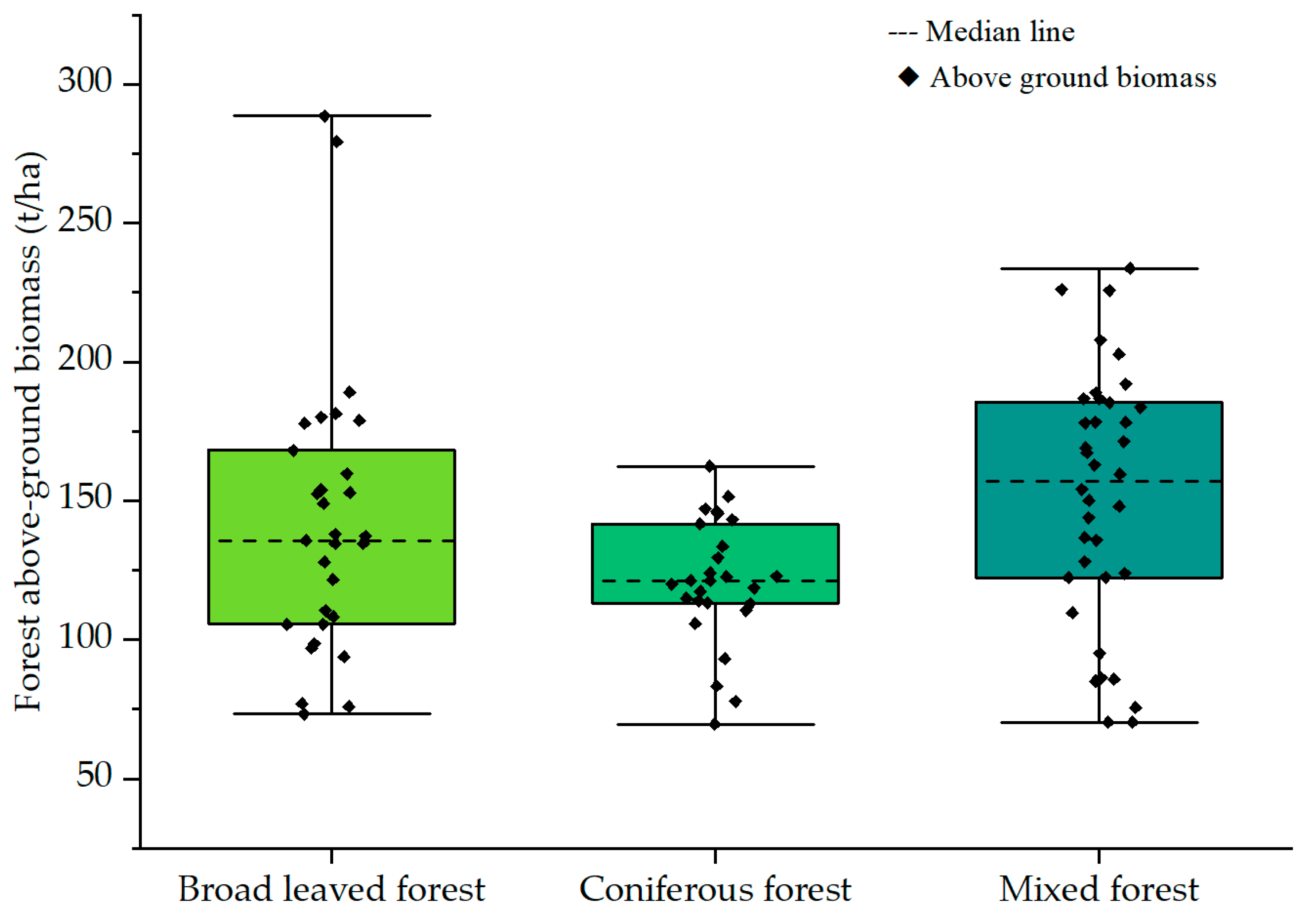
2.2. Field Data Collection and Processing

Sample plots in the study area were surveyed in December 2020, with a total of 96 standard plots, with a sample size of 20 m × 20 m. Diameter at breast height (DBH), tree height, and forest crown density were measured for all tree species in the sample plots, and only trees with DBH of 5 cm or above were measured. There were 27 coniferous forests, 31 broad-leaved forests, and 38 mixed forest sample plots. The AGB of the individual trees involved in each sample plot was calculated using the allometric equations shown in Table 1 [26]. The individual wood AGB in each sample plot was summed to obtain the total forest AGB for each plot, which was subsequently divided by the sample plot area to obtain the AGB per unit area of the sample plot and then converted to AGB per hectare (t/ha). Figure 2 illustrates the distribution of forest AGB statistics in the survey sample sites.

2.3. RS Data Collection and Processing

The Sentinel-1 (S1) data used in this study are Ground Range Detected (GRD) data with a pixel size of 10 m, a central incidence angle of 39.34°, and were obtained from the Copernicus Data Space Ecosystem (https://dataspace.copernicus.eu/, accessed on 9 November 2020). Sentinel-2 L2A (S2) data with a cloud cover of less than 2% were also obtained from the Copernicus Data Space Ecosystem (https://dataspace.copernicus.eu/, accessed on 10 November 2020). The Landsat 8 OLI (LT8) data used, with 3.73% cloud cover and a spatial resolution of 30 m, were obtained from the Geospatial Data Cloud (https://www.gscloud.cn/, accessed on 12 February 2021). The preprocessing of S1 data was conducted using SNAP (version 10.0) software, which mainly carried out fine-track correction, radiometric correction, coherent spot filtering, topographic correction (SRTM DEM), decibelization, and cropping; S2 data preprocessing was performed by the official, and bands B2 to B8A were selected for analysis in this paper. In order to unify the resolution of the data, the resolution of the B5, B6, B7, and B8A bands was upgraded from 20 m to 10 m using nearest neighbor interpolation and cropping, performed through resampling with SNAP (version 10.0). Preprocessing of the LT8 data was carried out in ENVI (version 5.6), specifically for radiative corrections and atmospheric corrections, followed by resampling of the bands to 10 m resolution using nearest neighbor interpolation and then cropping.

2.4. RS Feature Extraction

Based on the above preprocessed data, backscattering coefficients, vegetation indices, spectral information, and texture features were extracted, respectively, with reference to existing studies [27,28,29]. Among the texture features eight features with window sizes of 3 × 3, 5 × 5, 7 × 7, and 9 × 9 were computed using the gray level covariance matrix (GLCM), and the specific extracted RS features are shown in Table 2.

2.5. Feature Optimization and Model Building

Feature selection is a key step in forest AGB inversion using RS data. Selecting appropriate features from a large number of remotely sensed features can not only improve the accuracy of forest AGB inversion but also reduce the computation time of the estimation model. RF is a machine learning algorithm proposed by Breiman Leo in 2001 [30]. RS feature preference using RF is essentially a ranking of the importance of features. The importance of features in the input model is determined in the RF algorithm mainly by two metrics, the model MSE increment (%IncMSE) when the independent variable is used as out-of-bag data and the node purity of the model tree (IncNodePurity). Larger parameter values for these two metrics mean that the feature is more important. In this paper, the % IncMSE indicator is used as the main basis for selecting the top 10 variables for the construction of the models [31].
In this paper, three models, RF, SVR, and XGBoost, are used for the inversion of forest AGB, and the model parameters are optimized through grid search by setting different step values and exhaustively evaluating all parameter combinations to select the optimal model parameters. The specific implementation uses the caret package in the R langua (version R-4.4.0) for model construction, parameter tuning, and accuracy verification. In RF models, ntree represents the number of trees, and in general, the more trees the more stable the model will be, but it will increase the computational cost accordingly. mrty can control how many features per tree are used for evaluation when splitting, with a default choice of one-third. For RF parameters, we refer to the literature of [32,33,34] and perform a grid search. We perform the RF model using the randomForest package (version 4.7-1.1), and the regulated parameters are ntree and mrty. In this paper’s experiments, the range of ntree is between 10 and 200, with a step of 10 each time, and the range of mrty is between 1 and 10, with a step of 1 each time. In the SVR model, C is the regularization parameter that controls the degree of model fit. A model with too large a value of C may be overfitted, while a model with too small a value of C may be underfitted. The sigma, on the other hand, is an important parameter of the RBF that affects the nonlinear fitting ability of the model. Too small a parameter may lead to overfitting of the model and too large a parameter may lead to underfitting of the model. The RBF, on the other hand, is the most commonly used kernel function in SVR for situations where the data have nonlinear relationships. For SVR parameters, we refer to the literature of [35,36] and perform a grid search. We constructed the SVR model using the kernlab package (version 0.9-32), the kernel function is a radial basis function kernel, and the parameters for regulation are sigma and C. The range of sigma is 0.1 to 2 with 0.1 step at a time, and the range of C is 0.1 to 3.2 with 0.1 step at a time. In the XGBoost model, nrounds represents the total number of trees trained during the gradient boosting process. max_depth controls the complexity of the trees. eta represents the learning rate, which controls how much each tree contributes to the model. The gamma, on the other hand, controls the minimum loss function drop required for each split. colsample_bytree controls the proportion of randomly selected features for each tree training, which can effectively avoid overfitting and increase the diversity of the model. min_child_weight controls the minimum sample weight of the leaf nodes of each tree. subsample controls the proportion of samples used for training each tree, which helps to prevent overfitting due to its introduction of randomness. For XGBoost parameters, this paper refers to the literature of [9] and performs a grid search. We implemented the XGBoost model using the xgboost package (version 1.7.7.1), and the parameters to be tuned are nrounds, max_depth, eta, gamma, colsample_bytree, min_child_weight, and subsample. The nrounds parameter ranges from 10 to 50 with a step of 10 each time, the max_depth parameter is 3, 6, and 9, the eta parameter is 0.01, 0.3, 0.5, and 1, the gamma parameter is 0, 0.1, and 0.3, the colsample_bytree parameter is 0.7 and 1, the min_child_weight parameters are 1, 3, and 5, and the subsample parameters are 0.6, 0.8, and 1, respectively.

2.6. Model Accuracy Assessment

After grouping the ground survey samples according to forest types, the sample size of each group is small, so this paper uses leave-one-out cross-validation (LOOCV) to evaluate the test of the model prediction effect. LOOCV retains only one sample at a time as a test set, all the remaining samples are used for training the model, and the process is repeated until all the samples are used as a test set, and the method can make an effective evaluation of the stability and reliability of the model.
In this paper, both root mean square error (RMSE), mean absolute error (MAE), and coefficient of determination (R2) are used as the evaluation metrics of the model, which are calculated as Equation (1), Equation (2), and Equation (3), respectively. A lower root mean square error and mean absolute error mean that the model has less estimation error and is more effective, while a higher coefficient of determination means that the model fits better.
R M S E = 1 n i = 1 n ( y i y ^ i ) 2
M A E = 1 n i = 1 n y i y ^ i
R 2 = 1 i = 1 n ( y i y ^ i ) 2 i = 1 n ( y i y ¯ i ) 2
where y i is the measured value of forest AGB, y ¯ i is the mean value of forest AGB, y ^ i is the predicted value of forest AGB, and n is the number of samples.

3. Results

In this paper, we first used the RF algorithm to optimize the RS features involved in the AGB inversion process of different data combinations in three forest types and analyzed the correlation between each selected RS feature. Based on this, the estimation of forest AGB was carried out using RF, SVR, and XGBoost models with each of the six data combinations (S1, S2, LT8, S1 + LT8, S1 + S2, S1 + S2 + LT8).

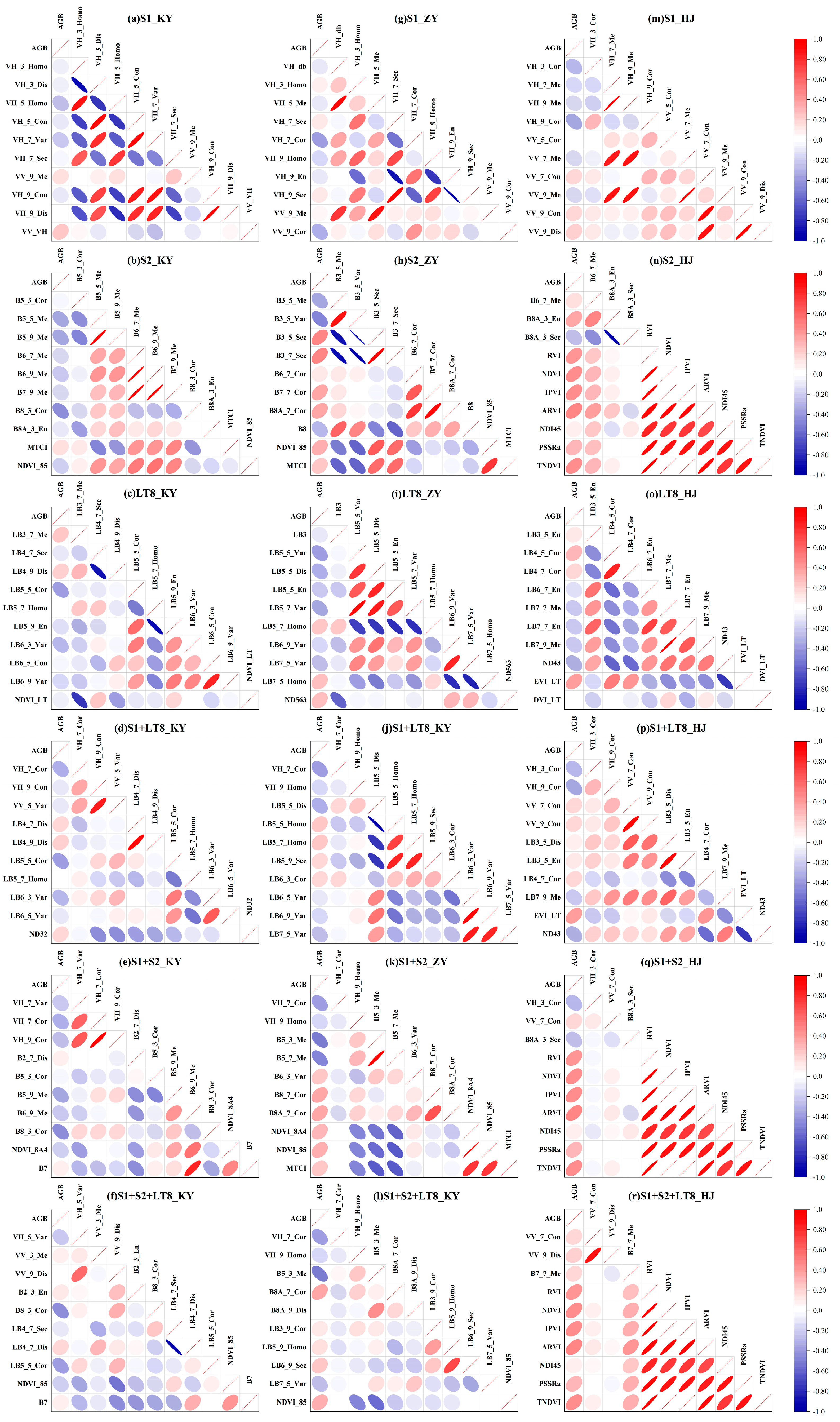
3.1. Feature Optimization Results and Analyses

Table 3 shows the results of the feature selection of different forest types AGB with different RS data combinations, and Figure 3 shows the features correlation of different forest types AGB with different remote sensing data combinations. As shown in Table 3, in broad-leaved forests, the VH texture characteristics of S1 are sensitive to broad-leaved forest AGB. The red-edge band texture features of S2, and the near- and short-wave infrared band texture features of LT8 are sensitive to broad-leaved forest AGB. In coniferous forests, the VH texture features of S1 were likewise more sensitive to AGB in coniferous forests, the green light, red-edge band, and near-infrared band texture features of S2 and their derived vegetation indices were more sensitive to AGB in coniferous forests, and the near-infrared and short-wave infrared band texture features of LT8 and their derived vegetation indices were more sensitive to AGB in coniferous forests. In mixed forests, the textural characteristics of VH and VV of S1 are sensitive to the mixed forest AGB. Vegetation indices derived from the red, red-edge, and near-infrared bands of S2, as well as textural features in the red-edge and near-infrared bands, are more sensitive to mixed forest AGB. LT8’s green light, textural characteristics in the short-wave infrared band, and its derived vegetation indices are more sensitive to mixed forest AGB. Overall, in S1 data, VH and its texture features are more sensitive to forest AGB. The reason for this is that S1 VH characterizes forest canopy scattering, while S1 VV characterizes ground scattering. Therefore, VH is more sensitive to forest canopy structural information compared to VV, and its texture features play a more significant role in feature selection [37,38].
In the multispectral data, the textural features of B5, B6, B7, B8, B8A red edge, near-infrared bands, and their derived vegetation indices of S2 are more predominant in comparison with the textural features of LB5, LB6, LB7 near-infrared bands, and short-wave infrared bands of LT8 compared to other features. The reason for this is that green vegetation has a strong reflection of NIR, while NIR is more sensitive to the foliar biomass of vegetation, and the red-edge band is between the NIR and red light bands, which is sensitive to small changes in the chlorophyll of green vegetation, and the growth status of vegetation [39,40]. Among the preferred features, texture features have the highest percentage because texture features contain the correlation between image elements and can further characterize the correlation between forest AGB and RS features [5]. Among the textural features, mean (Me) and contrast (Cor) appeared most frequently, which are effective in capturing changes in plant canopy structure and texture that have a correlation with biomass, and thus, these parameters accounted for more compared to other textural parameters [41]. The choice of texture window size is an important part of the texture feature computation. A window that is too small results in increased spectral variance within the window, which in turn enhances the noise; if the window is too large, the texture within the window is too smooth, resulting in texture information not being extracted efficiently [7,42]. Among the various data sources in this study, the 7 × 7 and 9 × 9 windows have a higher percentage of texture features, so the texture feature information extracted under this window is better for characterizing the structural information of the subtropical forest in Simao District relative to other windows.
Some of the textural features of B8 and B8A in S2 and their derived vegetation indices correlate well with all three forest AGB; some of the textural features of B4, B5, B6, and B7 in LT8 correlate well for all three forest AGB. As can be seen from Figure 3a–f, the high correlation between S1_KY features is more obvious in broad-leaved forests, and the situation is less in other data sets; from Figure 3g–l, it can be seen that in coniferous forests, there are more features with high correlation in a single data source, while the situation is reduced in the joint data; from Figure 3m–r, it can be seen that the correlation of the features screened by S2 data in the mixed forest is better for the AGB of the mixed forest, but the high correlation situation between the features is higher compared to S1, LT8, and S1 + LT8. The reason for this may be because RF performs feature filtering by evaluating the importance of each feature in all the trees and calculating its contribution in the split nodes, so that a feature may still be selected even if there is a correlation between the features. In addition, most of the correlated features are either from the same band or calculated from the red, red-edge, near-infrared, and short-wave infrared bands, which further exacerbates the occurrence of high correlation between features. Overall, the high feature-to-feature correlation is reduced in the joint data combination, which indicates that the redundant information can be reduced by combining SAR data and multispectral data, and the feature independence can be improved to enhance the performance of the model.

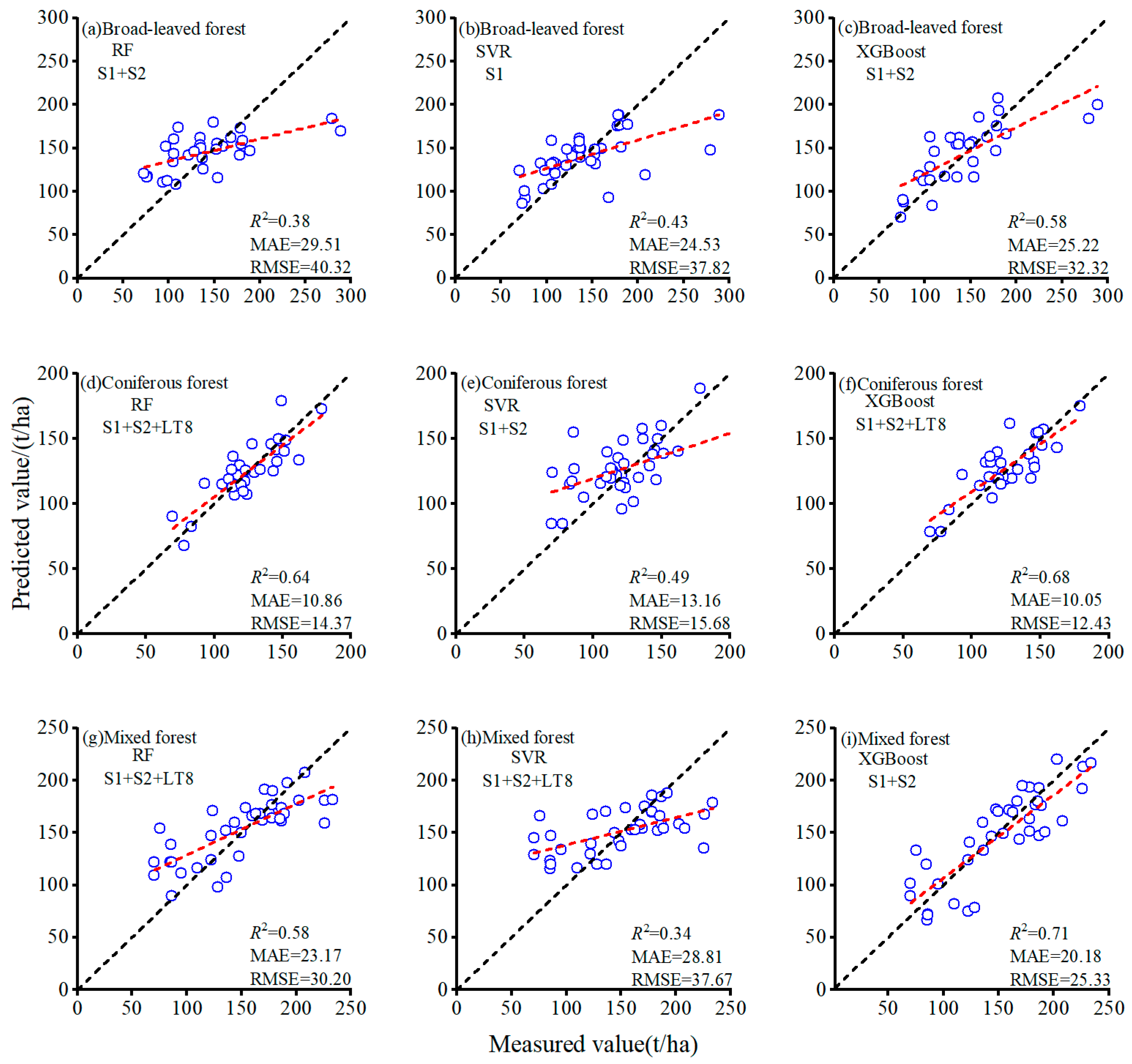
3.2. AGB Model Inversion Results and Analysis

Based on feature optimization, this paper constructs AGB inversion models for different forest types using the RF, SVR, and XGBoost models under the conditions of S1, S2, LT8, and combined data. The results, obtained using leave-one-out cross-validation, are presented in Table 4.
In broad-leaved forests, R2 ranged from 0.12 to 0.38, MAE ranged from 29.51 to 34.76 t/ha, and RMSE ranged from 40.32 to 46.61 t/ha using the RF model inversion, with the highest accuracy being for the S1 + S2 data combination (R2 = 0.38, MAE = 29.51 t/ha, RMSE = 40.32 t/ha). The R2 for SVR ranged from 0.18 to 0.60, MAE ranged from 24.53 to 39.14 t/ha, and RMSE ranged from 37.82 to 52.43 t/ha, with the lowest RMSE for the S1 data (R2 = 0.43, MAE = 24.53 t/ha, RMSE = 37.82 t/ha). The R2 of XGBoost ranged from 0.22 to 0.58, MAE ranged from 25.22 to 33.38 t/ha, and RMSE ranged from 32.32 to 44.44 t/ha, with the highest accuracy for the data combination of S1 + S2 (R2 = 0.58, MAE = 25.22 t/ha, RMSE = 32.32 t/ha). Overall, the XGBoost model combined with the S1 + S2 data had the lowest RMSE in inverting the broadleaf forest AGB, so we concluded that the XGBoost inversion accuracy was the best.
In coniferous forests, R2 ranged from 0.11 to 0.64, MAE ranged from 10.86 to 17.27 t/ha, and RMSE ranged from 14.37 to 21.26 t/ha using the RF model inversion, with the highest accuracy for the combination of S1 + S2 + LT8 data (R2 = 0.64, MAE = 10.86 t/ha, RMSE = 14.37 t/ha). The R2 for SVR ranged from 0.36 to 0.62, MAE ranged from 13.16 to 16.89 t/ha, and RMSE ranged from 15.68 to 22.49 t/ha, with the lowest RMSE for the S1 + S2 dataset (R2 = 0.49, MAE = 13.16 t/ha, RMSE = 15.68 t/ha). The R2 of XGBoost ranged from 0.28 to 0.68, MAE ranged from 10.05 to 17.45 t/ha, and RMSE ranged from 12.43 to 20.20 t/ha, with the highest R2 and lowest RMSE accuracy for the data combination of S1 + S2 + LT8 (R2 = 0.68, MAE = 10.05 t/ha, RMSE = 12.43 t/ha). Overall, the XGBoost model combined with S1 + S2 + LT8 data had the highest accuracy in inverting coniferous forest AGB.
In mixed forests, the R2 using the RF model inversion ranged from 0.27 to 0.58, MAE ranged from 23.17 to 32.80 t/ha, and RMSE ranged from 30.20 to 39.73 t/ha, with the highest accuracy of R2 and RMSE for the combination of S1 + S2 + LT8 data (R2 = 0.58, MAE = 23.17 t/ha, RMSE = 30.20 t/ha). The R2 of SVR ranged from 0.13 to 0.34, MAE ranged from 28.81 to 36.29 t/ha, and RMSE ranged from 37.67 to 42.75 t/ha, with the highest accuracy of R2 and RMSE for the combination of S1 + S2 + LT8 data (R2 = 0.34, MAE = 28.81 t/ha, RMSE = 37.67 t/ha). The R2 of XGBoost ranged from 0.28 to 0.71, MAE ranged from 21.37 to 31.68 t/ha, and RMSE ranged from 25.33 to 39.86 t/ha, with the highest R2 and RMSE accuracy for the S1 + S2 data combination (R2 = 0.71, MAE = 21.37 t/ha, RMSE = 25.33 t/ha). Taken together, the XGBoost model combined with S1 + S2 data had the highest accuracy in inverting the mixed forest AGB.
Figure 4 shows the scatterplot of the optimal results of the inversion of the three machine-learning models using different combinations of data in different forest types. In broad-leaved forests, the three machine learning models showed a high underestimation of forest AGB near 200 t/ha, which was more obvious for the RF and SVR models, and the XGBoost model improved compared to the RF and SVR situation. At forest AGB 100 t/ha and below, the RF and SVR models have a slight underestimation, whereas the XGBoost model is close to the measured values in this range and the underestimation is not significant. In coniferous forests, the three machine learning models showed high value underestimation at forest AGB near 150 t/ha, the XGBoost model performed better compared to the RF and SVR models, and in terms of low value overestimation, the SVR model performed worse than the RF and XGBoost models. In mixed forests, the RF and SVR models underestimated the high values of forest AGB > 200 t/ha, while the XGBoost model also showed this phenomenon, but the situation was improved compared with the RF and SVR models; at forest AGB 100 t/ha and below, all three models showed low value overestimation, but the XGBoost model still performed well, with a similar trend to the high-value underestimation.
In terms of fitting results, the RF model in broad-leaved forests fitted the worst, the distribution of forest AGB points around the 1:1 line was more dispersed, the SVR model fitted slightly better compared to the RF model, and the XGBoost model fitted the best. In the coniferous forest, the SVR model had the worst fit, the RF and XGBoost models had a better fit, and the forest AGB points were distributed around the 1:1 line overall. In the mixed forest, the SVR model had the worst fit, the RF model had an improved fit compared to the SVR model, and the XGBoost model had the best fit. In terms of saturation point, in broad-leaved forests, the saturation point of RF and SVR models is near 200 t/ha, and XGBoost model is near 250 t/ha. In coniferous forests, the saturation point of the SVR model was roughly above 150 t/ha, and the RF and XGBoost models did not have a clearer saturation point. In the mixed forest, the saturation point of all three models appeared near the forest AGB of 200 t/ha, but the XGBoost model tended to be stable compared to the RF and SVR models.
In a comprehensive analysis, XGBoost combined with SAR and multispectral data showed optimal accuracy in AGB inversion for broad-leaved forests, coniferous forests, and mixed forests. The reason for this is that the forest structure information reflected by S1 complements the forest canopy structure information reflected by S2 and LT8, which increases the saturation point of the forest AGB estimation, thus improving the inversion accuracy of the forest AGB. High-value underestimation and low-value overestimation occurred in this inversion in RF, SVR, and XGBoost, but XGBoost performed relatively lightly and its accuracy was significantly better than that of the RF and SVR models. This may be due to the gradient optimization mechanism of XGBoost, the adjustment of second-order derivatives, and the effective regularization strategy.

4. Discussion

4.1. Effects of Remote Sensing Variables on AGB in Subtropical Forests

In terms of RS features, a combination of the three forest-type features optimization results shows that VH and its texture features are more sensitive to forest AGB in S1 data. In the multispectral data, the texture features of B5, B6, B7, B8, B8A red edge, NIR bands and their derived vegetation indices of S2 and LB5, LB6, LB7 NIR bands and short-wave infrared bands of LT8 are more sensitive to the forest AGB in comparison with the other features. Tian [2] used S1 and S2 data to estimate subtropical forest AGB, and the results showed that VH and its texture features in S1 were selected more often compared to VV and its texture features in feature optimization, which confirmed that VH in S1 was more sensitive to forest AGB compared to VV. This is the same as the results of the present study, suggesting that the cross-polarised backward scattering feature is strongly correlated with the forest AGB. Zhang et al. [43] used S2 data for the estimation of subtropical forest AGB, and the results showed that the vegetation indices calculated based on the red-edge and near-infrared bands were more sensitive to forest AGB, which indicated that the red-edge and near-infrared bands of S2 were more relevant to forest AGB. Xu [44] used S1 and LT8 data for subtropical forest AGB inversion, and the results showed that the VH and its texture features in S1 data and the red band, infrared band and its texture features in LT8 have important roles in forest AGB inversion. The results of all the above studies are similar to the results of our study, further confirming that the VH, red edge, and infrared bands are more sensitive to forest AGB and have better correlation.

4.2. Impact of Different Machine Learning Models on Forest AGB

In terms of machine learning, this paper uses three machine learning models, RF, SVR, and XGBoost, for the construction of forest AGB inversion models. Among them, the inversion accuracy of XGBoost combined with SAR data and multispectral data was the highest among all three forest types. Li et al. [45] employed four models—MLR, RF, SVR, and XGBoost—to invert the AGB of sub-boreal zone forests using airborne LiDAR data and field survey data. The results indicated that the XGBoost model outperformed the other three models, achieving an R2 of 0.83. Li et al. [46] utilized S1, S2, PALSAR, and DEM data combined with RF and XGBoost models to estimate forest AGB in the sub-boreal region of China. The results demonstrated that the highest estimation accuracy was achieved using the XGBoost model, with an R2 of 0.67. Yan et al. [47] constructed a forest AGB estimation model for subtropical plantation forests using LT8 data and employed MLR, KNN, RF, and XGBoost models, respectively. The results indicated that the XGBoost model provided the best fitting and prediction results, with an R2 of 0.75. Li et al. [9] used S1 and LT8 data combined with LR, RF, and XGBoost models to invert forest AGB in the subtropical region of Hunan Province. The results showed that the XGBoost model combined with S1 + LT8 data achieved the highest inversion accuracy, with an R2 of 0.75. Additionally, compared with the other models, XGBoost effectively reduced the underestimation of high values and the overestimation of low values. XGBoost enhances the optimization efficiency of the loss function through a second-order Taylor expansion and incorporates a regularization strategy to effectively prevent overfitting. During the tree splitting process, if there are negative loss branches, XGBoost is able to automatically eliminate these branches to optimize the model structure. In addition, the splitting is based on the loss function and second-order derivatives for accurate splitting, which may be the reason why it outperforms RF and SVR in dealing with high value underestimation and low value overestimation problems. The results of the above studies in the sub-boreal and subtropical regions are similar to ours, indicating that the XGBoost algorithm has higher accuracy, better data applicability, and better model robustness in inverting machine learning models of forest AGB.

4.3. Impact of Remote Sensing Data Sources on Forest AGB

In terms of data source combinations, the inversion accuracies of the S1 + S2 and S1 + S2 + LT8 data combinations are better than the other data sets. Pan et al. [5] used S1 and S2 data for the estimation of forest AGB, and the results showed that the joint S1 + S2 data had the best estimation with an R2 of 0.57. David et al. [48] used S1 and S2 data combined with ML and RF for dryland forest AGB estimation, and the results showed that the S1 + S2 data set could estimate dryland forest AGB well with an R2 of 0.95. The results of the above studies are similar to the results of our study, i.e., the combination of multispectral data and SAR data can improve the inversion accuracy of forest AGB to a greater extent. However, it has to be noted that the inversion of the S1 + LT8 combination in this study is not as good as that of S1 + S2 and S1 + S2 + LT8. The reason may be that the spatial resolution of S2 is higher than that of LT8, and the ability of spectral feature variation, spatial information richness, and texture information of S2 images are richer compared to LT8, which improves the estimation of forest AGB to some extent [49].
Zhang et al. [50] Estimation of subtropical forest AGB using SVR, MLPNN, KNN, and RF models based on forest AGB maps derived from S1 + S2 data and LiDAR data. The results showed the best RF model estimation based on S1 + S2 data with R2 = 0.72, RMSE = 28.63 t/ha. Zhou et al. [4] Estimation of subtropical forest AGB in Taiping Lake, Anhui, China based on S1 + S2 data. The results showed that the joint S1 + S2 data had the highest estimation accuracy (R2 = 0.69, RMSE = 34.17 mg/hm2). The estimation results of the above studies are similar to the estimation results of this paper. The reason for the higher accuracy of RMSE in this paper is that this paper categorizes the forests. Therefore, the forest AGB estimation model in this paper has some generalizability in the estimation of AGB in other subtropical forests.
This paper focuses primarily on remotely sensed data and machine learning models, but climatic factors such as precipitation and temperature also have an impact on forest AGB. Climate factors regulate stand structure in forests, e.g., precipitation can promote tree diameter at breast height (DBH) and temperature can drive photosynthesis and thus forest AGB [51]. Therefore, RS data can be utilized to obtain climate factors such as precipitation and temperature when estimating forest AGB using machine learning models. And feature preference methods such as Random Forest Importance Ranking can be used to analyze the extent to which climate factors contribute to the construction of forest AGB models in the region. Although this paper combines SAR and multispectral data for complementary forest structural information, there are still deficiencies in forest AGB inversion studies. First of all, in SAR data, S1 is short-wave data in the C-band, which has weak penetration capability and cannot fully reflect the forest structure information in densely forested areas. Meanwhile, the saturation point of AGB is easily reached in the high forest AGB region, which affects the estimation accuracy, and the use of long-wave SAR data can be considered to improve the accuracy later. Second, while the combination of SAR and multispectral data improves the estimated saturation point of the forest AGB, saturation still occurs in high forest AGB regions. Additionally, when using the constructed model for large-scale forest AGB mapping, significant discrepancies may appear. The reason for this is the neglect of spatial autocorrelation in the sample data, which leads to overly optimistic model estimates. Therefore, the spatial autocorrelation between the samples should also be further investigated and analyzed when the sample data allow.

5. Conclusions

In this paper, we comprehensively used three kinds of data, Sentinel-1 (S1), Sentinel-2 (S2) and Landsat 8 (LT8), for different forest types in the subtropical area of Simao District, and used three models, RF, SVR, and XGBoost, to carry out forest AGB inversion, and obtained the following conclusions: (1) In the inversion of forest AGB, the VH of SAR data and the red edge and infrared bands of multispectral data have a strong sensitivity to the inversion of forest AGB, and further integration of the texture factors formed by these sensitive bands can invert forest AGB more accurately. (2) The machine learning model has high value underestimation and low value overestimation when inverting all the—three forest type AGB, which can be mitigated to some extent by the XGBoost algorithm. And XGBoost has the best fit, the strongest robustness, the weakest dependence on forest type, and the highest forest accuracy when combining SAR and multispectral data. In broad leaved forests R2 = 0.58, MAE = 25.22 t/ha, RMSE = 32.32 t/ha, in coniferous forests R2 = 0.68, MAE = 10.05 t/ha, RMSE = 12.43 t/ha, and in mixed forests, R2 = 0.71, MAE = 21.37 t/ha, RMSE = 25.33 t/ha. (3) The joint S1 + S2 data gave the best results for the inversion of AGB of the broad-leaved forests and mixed forests in subtropical forests in Simao District, Pu’er City, Yunnan Province, and the joint S1 + S2 + LT8 data gave the best results for the inversion of AGB of coniferous forests. (4) The spatial autocorrelation of the samples themselves should be taken into account when constructing a forest AGB estimation model when the sample data allow it.

Author Contributions

Conceptualization, Y.J. and Y.W.; methodology, Y.W.; software, Y.W., H.Z. and M.W.; validation, Y.W. and M.W.; resources, Y.J.; writing—original draft preparation, Y.W. and Y.J.; writing—review and editing, S.H., W.D. and Y.J.; visualization, Y.W. and H.Z.; supervision, Y.J. and M.W.; project administration, Y.J. All authors have read and agreed to the published version of the manuscript.

Funding

This research was funded by the National Natural Science Foundation of China under grant numbers 42161059, 32160365, 32371869, and 32471865, as well as by the Agriculture Joint Special Project of Yunnan Province under grant numbers 202301BD070001-058 and 202401BB070001-021.

Data Availability Statement

Sentinel-1 and Sentinel-2 data are available for downloading through the Copernicus Data Space platform (https://dataspace.copernicus.eu/, accessed on 9 November 2020 and 10 November 2020, respectively). Landsat 8 OLI data are available for downloading through the Geospatial Data Cloud platform (https://www.gscloud.cn/, accessed on 12 February 2021). Field-collected data are available and can be obtained by contacting the corresponding author.

Acknowledgments

The authors would like to thank everyone who helped to improve the quality of the manuscripts.

Conflicts of Interest

The authors declare no conflicts of interest.

References

  1. Li, D.; Wang, C.; Hu, Y.; Liu, S. General Review on Remote Sensing-Based Biomass Estimation. Geomat. Inf. Sci. Wuhan Univ. 2012, 37, 631–635. [Google Scholar]
  2. Tian, C. Remote Sensing Estimation of Aboveground Biomass in Subtropical Forests Based on Active Remote Sensing Data, Passive Remote Sensing Data, and Spaceborne LiDAR Data—A Case Study of Chenzhou City, Hunan Province. Master’s Thesis, Nanjing Forestry University, Nanjing, China, 2023. [Google Scholar]
  3. Xu, Z.; Li, C.; Li, M.; Li, C.; Wang, L. Forest Biomass Retrieval Based on Sentinel-1a and Landsat 8 Image. J. Cent. South Univ. For. Technol. 2020, 40, 147–155. [Google Scholar]
  4. Zhou, W.; Lv, Y.; Lin, Q. Retrieval of Above-ground biomass in Taiping Lake Forests Using Optical and SAR Dataset. J. Northwest For. Univ. 2023, 38, 193–200. [Google Scholar]
  5. Pan, L.; Sun, Y.; Wang, Y.; Chen, L.; Cao, Y. Estimation of Aboveground Biomass in a Chinese Fir (Cunninghamia lanceolata) Forest Combining Data of Sentinel-1 and Sentinel-2. J. Nanjing For. Univ. 2020, 44, 149. [Google Scholar]
  6. Hao, Q.; Huang, C. A Review of Forest Aboveground Biomass Estimation Based on Remote Sensing Data. Chin. J. Plant Ecol. 2023, 47, 1356. [Google Scholar] [CrossRef]
  7. Yan, H.; Jiang, X.; Wang, W.; Wu, Z.; Liu, F.; Wei, Y. Aboveground Biomass Inversion Based on Sentinel-2 Remote Sensing Images in Chongli District. J. Cent. South Univ. For. Technol. 2024, 44, 53–61. [Google Scholar]
  8. Liu, Q.; Yang, L.; Liu, Q.; Li, J. Review of Forest above-ground biomass Inversion Methods Based on Remote Sensing Technology. Remote Sens. 2015, 19, 62–74. [Google Scholar] [CrossRef]
  9. Li, Y.; Li, M.; Li, C.; Liu, Z. Forest Aboveground Biomass Estimation Using Landsat 8 and Sentinel-1a Data with Machine Learning Algorithms. Sci. Rep. 2020, 10, 9952. [Google Scholar] [CrossRef]
  10. Zhang, W.; Zhao, L.; Li, Y.; Shi, J.; Yan, M.; Ji, Y. Forest above-Ground Biomass Inversion Using Optical and Sar Images Based on a Multi-Step Feature Optimized Inversion Model. Remote Sens. 2022, 14, 1608. [Google Scholar] [CrossRef]
  11. Ding, J.; Huang, W.; Liu, Y.; Hu, Y. Estimation of Forest Aboveground Biomass in Northwest Hunan Province Based on Machine Learning and Multi-Source Data. Sci. Silvae Sin. 2021, 57, 36–48. [Google Scholar]
  12. Ji, Y.; Zhang, W.; Xu, K.; Ju, Y.; Li, W.; Jing, Q.; Wang, L.; Li, Y. Estimation of Forest Aboveground Biomass Based on Gf-3 Quad-Polarization Sar Data. Remote Sens. Technol. Appl. 2023, 38, 362–371. [Google Scholar]
  13. Guo, Y. Optimu Non-Parametric Method for Forest Above-Ground Biomass Estimation Based on Remote Sensing Data. Ph.D. Thesis, Chinese Academy of Forestry, Beijing, China, 2012. [Google Scholar]
  14. Gao, Y.; Lu, D.; Li, G.; Wang, G.; Chen, Q.; Liu, L.; Li, D. Comparative Analysis of Modeling Algorithms for Forest Aboveground Biomass Estimation in a Subtropical Region. Remote Sens. 2018, 10, 627. [Google Scholar] [CrossRef]
  15. Rodríguez-Veiga, P.; Quegan, S.; Carreiras, J.; Persson, H.J.; Fransson, J.E.S.; Hoscilo, A.; Ziółkowski, D.; Krzysztof, S.; Lohberger, S.; Matthias, S. Forest Biomass Retrieval Approaches from Earth Observation in Different Biomes. Int. J. Appl. Earth Obs. Geoinf. 2019, 77, 53–68. [Google Scholar] [CrossRef]
  16. Ou, G.; Li, C.; Lv, Y.; Wei, A.; Xiong, H.; Xu, H.; Wang, G. Improving Aboveground Biomass Estimation of Pinus Densata Forests in Yunnan Using Landsat 8 Imagery by Incorporating Age Dummy Variable and Method Comparison. Remote Sens. 2019, 11, 738. [Google Scholar] [CrossRef]
  17. Zhang, L.; Shao, Z.; Liu, J.; Cheng, Q. Deep Learning Based Retrieval of Forest Aboveground Biomass from Combined Lidar and Landsat 8 Data. Remote Sens. 2019, 11, 1459. [Google Scholar] [CrossRef]
  18. Awad, M.M. Flexiblenet: A New Lightweight Convolutional Neural Network Model for Estimating Carbon Sequestration Qualitatively Using Remote Sensing. Remote Sens. 2023, 15, 272. [Google Scholar] [CrossRef]
  19. Zadbagher, E.; Marangoz, A.; Becek, K. Estimation of above-Ground Biomass Using Machine Learning Approaches with Insar and Lidar Data in Tropical Peat Swamp Forest of Brunei Darussalam. iForest Biogeosci. For. 2024, 17, 172–179. [Google Scholar] [CrossRef]
  20. Fang, K.; Wu, J.; Zhu, J.; Xie, B. A Review of Technologies on Random Forests. J. Stat. Inf. 2011, 26, 32–38. [Google Scholar]
  21. Tan, Y.; Tian, Y.; Haung, Z.; Zhang, Q.; Tao, J.; Liu, H.; Yang, Y.; Zhang, Y.; Lin, J.; Deng, J. Aboveground Biomass of Sonneratia Apetala Mangroves in Mawei Sea of Beibu Gulf Based on Xgboost Machine Learning Algorithm. Acta Ecol. Sin. 2023, 43, 1–15. [Google Scholar]
  22. Wu, J.; Zhu, Y.; Jin, S.; Yang, T.; Feng, J.; Wu, Z.; Xue, T.; Jiang, Y. Area Prediction of Cyanobacterial Blooms Based on Three Machine Learning Methods in Taihu Lake. J. Hohai Univ. (Nat. Sci.) 2020, 48, 542–551. [Google Scholar]
  23. Liu, Y. Merged Airborne LiDAR and Hyperspectral Data for Tree Species Classification in Puer’s Mountainous Area. Master’s Thesis, Chinese Academy of Forestry, Beijing, China, 2016. [Google Scholar]
  24. Xu, M.; Wang, J.; Xu, H.; Ou, G. Relationship between Spatial Structure of Pinus Kesiya Var. Langbianensis Natural Forest and the above-Ground Biomass of Individual Trees. J. Yunnan Univ. Nat. Sci. Ed. 2020, 42, 364–373. [Google Scholar]
  25. Liu, X.; Ou, S.; Lu, S.; Yue, C. Estimation of Forest Volume Based on Sentinel-1a Microwave Remote Sensing Data. J. West China For. Sci. 2020, 49, 128–136. [Google Scholar]
  26. Xu, H.; Zhang, H. Study on Tree Biomass Models, 1st ed.; Hu, P., Sun, W., Eds.; Yunnan Science and Technology Press: Kunming, China, 2002. [Google Scholar]
  27. Yin, T.; Zhang, J.; Liao, Y.; Wang, F.; Gao, J.; He, Y.; Chen, C.; Xiao, Q. Estimating the Pinus Densata Carbon Storage of Shangri-La by Environmental Variables. J. West China For. Sci. 2024, 53, 119–128. [Google Scholar]
  28. Sun, X. Biomass Estimation Model of Pinus Densata Forests in Shangri-La City Based on Landsat8-Oli by Remote Sensing. Master’s Thesis, Southwest Forestry University, Kunming, China, 2016. [Google Scholar]
  29. Tian, C.; Li, M.; Li, T.; Li, D.; Tian, L. Estimation of Forest Net Primary Productivity Based on Sentinel Active and Passive Remote Sensing Data and Canopy Height. J. Nanjing For. Univ. 2024, 48, 132. [Google Scholar]
  30. Breiman, L. Random Forests. Mach. Learn. 2001, 45, 5–32. [Google Scholar] [CrossRef]
  31. Su, H.; Shen, W.; Wang, J.; Ali, A.; Li, M. Machine Learning and Geostatistical Approaches for Estimating Aboveground Biomass in Chinese Subtropical Forests. For. Ecosyst. 2020, 7, 64. [Google Scholar]
  32. Han, H.; Wan, R.; Li, B. Estimating Forest Aboveground Biomass Using Gaofen-1 Images, Sentinel-1 Images, and Machine Learning Algorithms: A Case Study of the Dabie Mountain Region, China. Remote Sens. 2022, 14, 176. [Google Scholar]
  33. Ma, J.; Zhang, W.; Ji, Y.; Huang, J.; Huang, G.; Wang, L. Total and Component Forest Aboveground Biomass Inversion Via Lidar-Derived Features and Machine Learning Algorithms. Front. Plant Sci. 2023, 14, 17. [Google Scholar]
  34. Pandit, S.; Tsuyuki, S.; Dube, T. Estimating above-Ground Biomass in Sub-Tropical Buffer Zone Community Forests, Nepal, Using Sentinel 2 Data. Remote Sens. 2018, 10, 601. [Google Scholar] [CrossRef]
  35. Wang, P.; Tan, S.; Zhang, G.; Wang, S.; Wu, X. Remote Sensing Estimation of Forest Aboveground Biomass Based on Lasso-Svr. Forests 2022, 13, 1597. [Google Scholar] [CrossRef]
  36. Zhang, Y.; Ma, J.; Liang, S.; Li, X.; Li, M. An Evaluation of Eight Machine Learning Regression Algorithms for Forest Aboveground Biomass Estimation from Multiple Satellite Data Products. Remote Sens. 2020, 12, 4015. [Google Scholar] [CrossRef]
  37. Vreugdenhil, M.; Wagner, W.; Bauer-Marschallinger, B.; Pfeil, I.; Teubner, I.; Rüdiger, C.; Strauss, P. Sensitivity of Sentinel-1 Backscatter to Vegetation Dynamics: An Austrian Case Study. Remote Sens. 2018, 10, 1396. [Google Scholar] [CrossRef]
  38. Gašparović, M.; Dobrinić, D. Comparative Assessment of Machine Learning Methods for Urban Vegetation Mapping Using Multitemporal Sentinel-1 Imagery. Remote Sens. 2020, 12, 1952. [Google Scholar] [CrossRef]
  39. Su, H.; Li, J.; Chen, X.; Liao, J.; Wen, D. Forest Biomass Based on the Forest Communities and Image Spectral Curve Character-Istics: A Remote Sensing Estimation in Fujian Province. Acta Ecol. Sin. 2016, 37, 5742–5755. [Google Scholar]
  40. Jiang, F.; Sun, H.; Li, C.; Ma, K.; Chen, S.; Long, J.; Ren, L. Retrieving the Forest Aboveground Biomass by Combining the Red Edge Bands of Sentinel-2 and Gf-6. Acta Ecol. Sin. 2021, 41, 8222–8236. [Google Scholar]
  41. Jian, Y.; Han, Z.; Huang, G.; Wang, X.; Li, Y.; Zhou, J.; Dian, Y. Estimation of Forest Biomass Using High Spatial Resolution Remote Sensing Imagery in North Subtropical Forests. Acta Ecol. Sin. 2021, 41, 2161–2169. [Google Scholar]
  42. Chen, L.; Hao, W.; Gao, D. The Latest Applications of Optical Image Texture in Forestry. J. Beijing For. Univ. 2015, 37, 1–12. [Google Scholar]
  43. Zhang, X.; Shen, H.; Huang, T.; Wu, Y.; Guo, B.; Liu, Z.; Luo, H.; Tang, J.; Zhou, H.; Wang, L. Improved Random Forest Algorithms for Increasing the Accuracy of Forest Aboveground Biomass Estimation Using Sentinel-2 Imagery. Ecol. Indic. 2024, 159, 111752. [Google Scholar]
  44. Xu, Z. Forest Biomass Retrieval Based on Sentinel-1a and Landsat 8 Image in Guidong County. Master’s Thesis, Nanjing Forestry University, Nanjing, China, 2020. [Google Scholar]
  45. Li, Y.; Peng, D.; Yuan, Y. Airborne Lidar Data Inversion of Forest Aboveground Biomass Using Xgboost Algorithm. J. Northeast Foresrty Univ. 2023, 51, 106–112. [Google Scholar]
  46. Li, J.; Bao, W.; Wang, X.; Song, Y.; Liao, T.; Xu, X.; Guo, M. Estimating Aboveground Biomass of Boreal Forests in Northern China Using Multiple Data Sets. IEEE Trans. Geosci. Remote Sens. 2024, 62, 4408410. [Google Scholar]
  47. Yan, Y.; Deng, Z.; Li, B.; Zhao, T. Estimation Models of Aboveground Biomass in Plantations Based on Landsat 8 Data. J. Northwest For. Univ. 2024, 39, 53–60, 77. [Google Scholar]
  48. David, R.M.; Rosser, J.; Donoghue, D. Improving above-ground biomass Estimates of Southern Africa Dryland Forests by Combining Sentinel-1 Sar and Sentinel-2 Multispectral Imagery. Remote Sens. Environ. 2022, 282, 113232. [Google Scholar] [CrossRef]
  49. Hang, T.; Ou, G.; Wu, Y.; Xu, X.; Wang, Z.; Lin, R.; Xu, C. Multi-source Remote Sensing Estimation of Forest Biomass Based on Machine Learning Algorithm. J. Northwest For. Univ. 2024, 39, 10–18. [Google Scholar]
  50. Zhang, L.; Zhang, X.; Shao, Z.; Jiang, W.; Gao, H. Integrating Sentinel-1 and 2 with Lidar Data to Estimate Aboveground Biomass of Subtropical Forests in Northeast Guangdong, China. Int. J. Digit. Earth 2023, 16, 158–182. [Google Scholar] [CrossRef]
  51. Ma, Y.; Eziz, A.; Halik, Ü.; Abliz, A.; Kurban, A. Precipitation and Temperature Influence the Relationship between Stand Structural Characteristics and Aboveground Biomass of Forests—A Meta-Analysis. Forests 2023, 14, 896. [Google Scholar] [CrossRef]
Figure 1. Overview of the study area. Note: (a) The figure shows the geographical location of Yunnan Province in China and also marks Pu’er City within Yunnan Province. (b) The figure indicates the geographic location of Simao District within Pu’er City and marks the location of the study area. (c) The figure depicts the geographic location of the ground-truthing sample plots in Simao District.
Forests 16 00559 g001
Figure 2. Overview of forest AGB in sample plots.
Forests 16 00559 g002
Figure 3. Correlation heat maps. Note: In the figure, KY represents broad-leaved forest, ZY is coniferous forest and HJ is mixed forest. On the color bar, 1 to −1 is the threshold for correlation; an ellipse facing the right is a positive correlation, and one facing the left is a negative correlation; a smaller ellipse represents a higher correlation, and vice versa for a lower correlation.
Forests 16 00559 g003
Figure 4. Cross-validation results. Note: In the figure, the red line represents the fitted line of the machine learning model. The black line represents the 1:1 line. The blue hollow circles represent the samples.
Forests 16 00559 g004
Table 1. Forest AGB models of various tree species in the study area.
Tree SpeciesAbove-Ground Biomass Models
Pinus kesiya var. langbianensis (A.Chev.) Gaussen ex Bui M = 0.0582 D H B 2.1203 H 0.4668
Schima superba Gardner & Champ. M = 0.12045 D H B 2.06446 H 0.38265
Eucalyptus robusta Sm. M = 0.814 ( D H B 2 H ) 0.9816
Cupressus funebris Endl. M = 0.010158 D H B 2.94424 H 0.41591
Cunninghamia lanceolata (Lamb.) Hook M = 0.10301 ( D H B 2 H ) 0.7773
Quercus × leana Nutt. M = 0.22999 D H B 1.39183 H 0.57393
Castanopsis fargesii Franch. M = 0.1355 ( D H B 2 H ) 0.817 + 0.0275 ( D H B 2 H ) 0.8165
Various kinds of birch in southwest China M = 0.08907 D H B 1.89807 H 0.52019
Hard broadleaved M = 0.3507 ( D H B 1.1948 ) 2 + ( 0.03017 D H B 2.3643 + 0.051 ) + ( 0.01813 D H B 2 0.2477 )
Soft broadleaved M = 0.02739 ( D H B 2 H ) 0.898869 + ( 0.01497 ( D H B 2 H ) 0.875639 + ( 0.01059 ( D H B 2 H ) 0.813953 ) + ( 0.0121 ( D H B 2 H ) 0.854295
Note: DHB is diameter at breast height, H is tree height, M is forest above-ground biomass.
Table 2. RS features.
Data SourceFeatures Name
S1Sigma0_VH/VV, VV_VH (VV-VH), VH_VV (VH+VV)
S2B2-B8A, ARVI, DVI, GEMI, GNDVI, IPVI, IRECI, MSAVI, MSAVI2, MTCI, NDVI, NDVI45, PSSRa, PVI, REIP, RVI, S2REP, SAVI, WDVI, TSAVI, TNDVI, EVI, NDVI85, NDVI86, NDVI87, NDVI8A4, NDVI8A5, NDVI8A6, NDVI8A7
L8B2-B7, DVI, NDVI, RVI, EVI, SAVI, ND32, ND43, ND67, ND452, ND563
S1/S2/LT8Bi_N_Me (Mean), Bi_N_Var (Variance), Bi_N_Homo (Homogeneity), Bi_N_Con (Contrast), Bi_N_Dis (Dissimilarity), Bi_N_En (Entropy), Bi_N_Sec (Second-order Moment), Bi_N_Cor (Correlation)
Note: Bi refers to LB2, LB3 … LB7 in LT8, and B2, B3 … B8A in S2; N represents the window size, with values of 3, 5, 7, and 9.
Table 3. Features selection results.
Forest TypeData SourceFeatures Name
Broad-leaved forestS1VH_3_Homo, VH_3_Dis, VH_5_Homo, VH_5_Con, VH_7_Var, VH_7_Sec, VV_9_Me, VH_9_Con, VH_9_Dis, VV_VH
S2B5_3_Cor, B5_5_Me, B5_9_Me, B6_7_Me, B6_9_Me, B7_9_Me, B8_3_Cor, B8A_3_En, MTCI, NDVI_85
LT8LB3_7_Me, LB4_7_Sec, LB4_9_Dis, LB5_5_Cor, LB5_7_Homo, LB5_9_En, LB6_3_Var, LB6_5_Con, LB6_9_Var, NDVI_LT
S1 + LT8VH_7_Cor, VH_9_Con, VV_5_Var, LB4_7_Dis, LB4_9_Dis, LB5_5_Cor, LB5_7_Homo, LB6_3_Var, LB6_5_Var, ND32
S1 + S2VH_7_Var, VH_7_Cor, VH_9_Cor, B2_7_Dis, B5_3_Cor, B5_9_Me, B6_9_Me, B8_3_Cor, NDVI_8A4, B7
S1 + S2 + LT8VH_5_Var, VV_3_Me, VV_9_Dis, B2_3_En, B8_3_Cor, LB4_7_Sec, LB4_7_Dis, LB5_5_Cor, NDVI_85, B7
Coniferous forestS1Sigma0_VH_db, VH_3_Homo, VH_5_Me, VH_7_Sec, VH_7_Cor, VH_9_Homo, VH_9_En, VH_9_Sec, VV_9_Me, VV_9_Cor
S2B3_5_Me, B3_5_Var, B3_5_Sec, B3_7_Sec, B6_7_Cor, B7_7_Cor, B8A_7_Cor, B8, NDVI_85, MTCI
LT8LB3, LB5_5_Var, LB5_5_Dis, LB5_5_En, LB5_7_Var, LB5_7_Homo, LB6_9_Var, LB7_5_Var, LB7_5_Homo, ND563
S1 + LT8VH_7_Cor, VH_9_Homo, LB5_5_Homo, LB5_5_Dis, LB5_7_Homo, LB5_9_Sec, LB6_3_Cor, LB6_5_Var, LB6_9_Var, LB7_5_Var
S1 + S2VH_7_Cor, VH_9_Homo, B5_3_Me, B5_7_Me, B6_3_Var, B8_7_Cor, B8A_7_Cor, NDVI_8A4, NDVI_85, MTCI
S1 + S2 + LT8VH_7_Cor, VH_9_Homo, B5_3_Me, B8A_7_Cor, B8A_9_Dis, LB3_9_Cor, LB5_9_Homo, LB6_9_Sec, LB7_5_Var, NDVI_85
Mixed forestS1VH_3_Cor, VH_7_Me, VH_9_Me, VH_9_Cor, VV_5_Cor, VV_7_Me, VV_7_Con, VV_9_Me, VV_9_Con, VV_9_Dis
S2B6_7_Me, B8A_3_En, B8A_3_Sec, RVI, NDVI, IPVI, ARVI, NDI45, PSSRa, TNDVI
LT8LB3_5_En, LB4_5_Cor, LB4_7_Cor, LB6_7_En, LB7_7_Me, LB7_7_En, LB7_9_Me, ND43, EVI_LT, DVI_LT
S1 + LT8VH_3_Cor, VH_9_Cor, VV_7_Con, VV_9_Con, LB3_5_Dis, LB3_5_En, LB4_7_Cor, LB7_9_Me, EVI_LT, ND43
S1 + S2VH_3_Cor, VV_7_Con, B8A_3_Sec, RVI, NDVI, IPVI, ARVI, NDI45, PSSRa, TNDVI
S1 + S2 + LT8VV_7_Con, VV_9_Dis, B7_7_Me, RVI, NDVI, IPVI, ARVI, NDI45, PSSRa, TNDVI
Note: XXX_LT is the vegetation index for LT8.In texture features, A_B_C, A denotes the band (VH, VV, Bi, LBi), B denotes the size of the texture window (3, 5, 7, 9), and C denotes the specific name in the texture feature.
Table 4. Models inversion accuracy.
Forest TypeData TypeModels
BLF RFSVRXGBoost
R2MAERMSER2MAERMSER2MAERMSE
S10.1733.7745.20.4324.5337.820.5227.9434.86
S20.2931.1742.980.3231.1741.190.4529.7236.87
LT80.2230.0144.250.3937.6351.250.2933.3842.43
S1L80.1234.7646.610.6039.1452.430.2231.6544.44
S1S20.3829.5140.320.3628.0039.660.5825.2232.32
S1S2L80.2832.5942.960.1832.1945.050.4429.1337.32
CF RFSVRXGBoost
R2MAERMSER2MAERMSER2MAERMSE
S10.5313.95 16.280.5716.80 22.340.6011.85 14.00
S20.4313.39 16.600.3613.88 17.660.5212.23 14.88
LT80.1117.27 21.260.6216.98 22.300.2817.45 20.20
S1L80.5911.83 14.720.4216.77 22.340.6111.05 13.69
S1S20.5513.50 16.080.4913.16 15.680.6210.91 13.52
S1S2L80.6410.86 14.370.5816.84 22.490.6810.05 12.43
MF RFSVRXGBoost
R2MAERMSER2MAERMSER2MAERMSE
S10.3230.88 39.130.2433.50 40.340.3330.7738.78
S20.4826.82 33.530.2230.94 40.480.5325.4631.25
LT80.2732.80 39.730.1734.56 41.600.2831.6839.86
S1L80.3430.07 37.530.1336.29 42.750.4929.4138.47
S1S20.5626.18 30.920.2431.06 39.860.7120.1825.33
S1S2L80.5823.17 30.200.3428.81 37.670.6721.3726.25
Note: BLF is broad-leaved forest; CF is coniferous forest; MF is mixed forest. MAE and RMSE units are tons per hectare (t/ha).
Disclaimer/Publisher’s Note: The statements, opinions and data contained in all publications are solely those of the individual author(s) and contributor(s) and not of MDPI and/or the editor(s). MDPI and/or the editor(s) disclaim responsibility for any injury to people or property resulting from any ideas, methods, instructions or products referred to in the content.

