Abstract
Distance to the pith is a parameter that is known to be correlated with the mechanical properties of wood, but it is not utilized in strength grading machines. This study aimed to investigate how different the mechanical properties and grading yields are for Douglas fir (Pseudotsuga menziesii (Mirb.) Franco) boards with small and large distances to the pith, respectively, and whether the distance to the pith could be an interesting parameter to use for strength grading in combination with other predictor variables. For this purpose, 221 boards were scanned to obtain fiber orientation and local density. Their dynamic modulus of elasticity and distance to the pith were measured, and they were finally tested in bending. The boards were classified into two categories: corewood if a board’s cross-section was entirely located within a radius of 200 mm from the pith, and outerwood otherwise. The results show that corewood presents lower mechanical properties than outerwood, explained especially by the higher knottiness of corewood. Distance to the pith improves the grading yields of a machine based on fiber orientation measurements, but using the dynamic modulus of elasticity rather than the distance to the pith leads to better results. Distance to the pith can be used as a single or secondary parameter to predict timber strength if the dynamic modulus of elasticity is not used.
1. Introduction
For various reasons, trees modify the properties of the wood fibers they produce. These variations are progressive and depend on the studied property (such as density, microfibril angle, cell dimensions, and mechanical properties), the species, the tree environment, etc. [1,2,3]. It is common to talk about juvenile and mature wood to designate the wood formed by a young cambium and an older one, respectively. The wording relative to corewood and outerwood refers more precisely to the radial gradients in properties, from pith to bark [2,4,5,6,7,8]. The most detailed terminology uses the terms juvenile corewood for the wood located near the pith at the base of the tree, but also mature corewood in the upper part of the tree [6,8]. The progression in the transition to juvenile corewood and mature outerwood is well-known; however, most authors in the literature define a boundary, which is between 5 and 20 growth rings from the pith [2,8]. Indeed, transition times are highly influenced by genetic and environmental factors [9,10]. In this study, the corewood/outerwood terminology will be used in relation to wood’s radial distance to the pith rather than the number of growth rings (both being highly correlated). The usage of the distance to the pith and the corewood/outerwood terminology is clear and possibly convenient in an industrial context because it relates to log diameter and the position of boards within the log rather than tree or board age.
Forestry practices tend toward short rotations and fast growth of trees, especially for softwoods in southern Europe such as Douglas fir (Pseudotsuga menziesii (Mirb.) Franco). Thus, these trees are often harvested when they have a relatively small diameter at breast height (mostly 40 cm or below), that is, when they are relatively young. The sawn structural timber obtained from this resource is, therefore, mainly made of corewood because, in the sawing process, only a small proportion of the wood material located in the outer radius of the log can be transformed into rectangular timber, with the rest being chipped. Issues related to high proportions of juvenile wood in timber from different species have been discussed by Kennedy [11]. This author reviewed several publications showing that the mechanical properties of juvenile wood of Douglas fir were inferior to those of mature wood. More recent results on Southern German Douglas fir quantify this behavior [12]: they show that for a planting density of 1000 trees per hectare, only 50% of corewood timber was machine-graded to C24, while 85% of the outerwood timber was graded as C24. However, there was no comparison between corewood and outerwood obtained from destructive mechanical tests in this study.
Machine strength grading is regulated in Europe by European standard EN 14081-2+A1 [13]. It is based on the statistical relationships between the so-called indicating properties (IPs) and each of the three grade-determining properties (GDPs), which are defined in terms of strength (in bending for C grades or in tension for T grades), modulus of elasticity (MoE), and density. The IPs are predictor variables or a combination of predictor variables based on non-destructive measures such as axial dynamic MoE, local density obtained by X-ray scanning, or fiber orientation scanning. While the dynamic MoE is a global measure of a board, local density and local fiber orientation allow the determination of the local variations in knottiness within a board and, ultimately, of the local stiffness and strength [14,15,16,17,18,19,20,21].
Kennedy [11] remarked that the distance to the pith was not taken into account in the visual grading standards for structural timber, which could result in overestimated mechanical properties for Douglas fir juvenile wood. Both Zobel et al. and Kennedy [1,11] concluded that the use of machine stress rating systems is needed to evaluate more precisely the mechanical properties of juvenile timber products. The most common principle of the existing nondestructive grading machines is to predict an MoE and assume that the bending strength is correlated with it, but several articles have shown that the bending strength of structural-size timber is more affected by the juvenile nature of wood than what the grade-determining MoE is [5,22]. Thus, it may be interesting to use distance to the pith or the cambial age of wood as a predictor of the strength. Corewood boards could be distinguished from outerwood boards according to a given distance to the pith automatically in a sawmilling industrial context by applying recently developed technologies based on optical scanning and annual ring detection [23,24,25]. Such method can also allow for determining the average annual ring width of a board, which is correlated to density and MoE and can be used as a predictor for strength grading [26]. While the distance to the pith is known to correlate with the mechanical properties of wood, its potential as a predictor variable for strength grading has not been extensively studied. This research aimed to fill this knowledge gap by investigating how the distance to the pith can be used in combination with other predictor variables to improve the accuracy of strength grading of Douglas fir timber.
In particular, the following objectives were included in this study:
- Investigate how different the GDPs of Douglas fir timber are between corewood and outerwood, and what the potential optimum yields of corewood and outerwood are, respectively, in the common strength classes.
- Investigate the grading accuracy obtained by using different machine strength grading methods when applied to boards of corewood and outerwood, respectively.
- Investigate whether the distance to the pith would be an interesting parameter to be used alone or in combination with other predictor variables obtained using common machines for strength grading in the IP predicting the bending strength.
These results aim to evaluate the engineering potential of boards according to the distance to the pith, and thereby contribute to the basis for decision-making for Douglas fir forest owners and the sawmilling industry regarding the suitable size of logs at the time of harvesting and the type of strength grading technology to use.
2. Materials and Methods
The main symbols and abbreviations used in this study are listed in Table 1.

Table 1.
List of the main abbreviations and variables.
2.1. Sampling
Eight logs of Douglas fir (Pseudotsuga menziesii (Mirb.) Franco) were selected from the common supply of a sawmill for their diameter of 50–55 cm. They were butt logs originating from different trees which had grown in France, and exhibited significant volumes of outerwood and boards with various distances to the pith. Butt end diameters and log cambial age are given in Table 2. From these logs, 241 boards were sawn and dried at an industrial sawmill, aiming for the same nominal dimensions of 40 × 100 × 3000 mm3. Between 24 and 36 boards per log were retrieved (Table 2).
Table 2.
Characteristics of the Douglas fir logs that were used.
2.2. Nondestructive and Destructive Testing of Boards
An industrial board scanner was used to measure board dimensions, local density, and local fiber orientation, while the boards were conveyed longitudinally. An industrial vibratory machine was used to determine dynamic MoE. Finally, a four-point bending test was performed to assess the bending strength and local and global bending MoE of the boards.
2.2.1. Moisture Content and Density
Board moisture content () was measured with a Gann HT 95 (Gerlingen, Germany) pin-type moisture meter at the time of the destructive test. The mean moisture content was 12.3% (standard deviation of 0.8%), with a minimum of 9.7% and a maximum of 14%; thus, all the boards complied with the EN 384+A2 [27] requirement of wood being between 8% and 18% of moisture content.
Board dimensions (, length, , thickness, and , width) were measured with the scanner by means of line lasers. These measurements allowed for computing each board’s average density after weighting each board with a scale. The grade-determining density of each board was obtained following the EN 384+A2 [27] requirements, by adjusting it to 12% moisture content and dividing it by 1.05 to match the density of small defect-free specimens (Equation (12)):
It should be noted that according to EN 384+A2 [27], the density that gives basis for the grade-determining density shall be determined as prescribed in EN 408+A1 [28] as the density of a specimen free of knots and resin pockets cut out as near as possible to the fracture zone after the destructive test. However, this was not performed in this study, and therefore, as defined above was used as the grade-determining density.
2.2.2. Moduli of Elasticity
The axial dynamic MoE of each board, , was obtained prior to the bending test using an industrial vibration machine. It determined the first longitudinal resonance frequency, with vibrations generated by a hammer impact, by means of a laser Doppler vibrometer located at one end of the board. Knowing the length and the average density of the board, its dynamic MoE was calculated as follows:
where is the length of the board, is the board density, and is the first axial resonance frequency.
In accordance with EN 408+A1 [28], the total span between the supports for the bending test was set to 18 times the nominal height of the board, i.e., 1800 mm, with the distance between each loading head and the closest support set to six times the depth of the board, i.e., 600 mm (Figure 1b). As stated in EN 384+A2 [27], the position of the board between the supports was chosen in order to have the expected weakest possible cross-section between the loading heads, which was possible in most cases since the boards were as long as 3000 mm (see Figure 1b). The position of the board in the test was recorded for each board, and boards were always oriented, both in the test and when fed into the scanner, so that the scanner data relative to the tested zone was known. The global MoE of each board directly computed from the bending test, , is as follows:
where is the span of the test (1800 mm here), is the distance between a loading position and the nearest support (600 mm here), is the thickness of each beam, is the height of each beam, and , respectively, are a higher and a lower levels of the total loading applied by the loading heads, and and , respectively, are the corresponding global deflections at the mid-point between the loading heads. G represents the shear modulus, here set to infinity as proposed in the European standards (shear deformations are implicitly taken into account in Equation (5)). The global MoE was also corrected with respect to moisture content in accordance with EN 384+A2 [27] as follows:
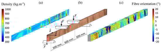
Figure 1.
(a) Two-dimensional map of local density obtained by X-ray scanning; (b) isometric view of the same board (image of the board captured by optical scanning) subjected to a 4-point bending test; (c) isometric view of the board showing angles between the local fiber direction and the longitudinal direction of the board (one narrow face and one wide face shown).
The global MoE was corrected to take into account the shear deformation as proposed in EN 384+A2 [27] to finally give the grade-determining MoE as follows:
with in GPa.
The local MoE observed during the bending test, , was also computed according to EN 408+A1 [28]. It was obtained using a device located between the loading heads, measuring the deflection in this pure bending zone along a length of five times the height of the beam, i.e., = 500 mm, as follows:
where is the second moment of the area. This local MoE was also corrected according to each board moisture content as proposed in EN 384+A2 [27]:
2.2.3. Bending Strength
The bending strength was calculated in accordance with EN 408+A1 [28] as follows:
where is the maximum value of the load applied by each loading head. It was also corrected according to EN 384+A2 [27] with respect to the size effect related to the height of the beam in the bending test (i.e., the width of each board). Thus, the following equation gives the grade-determining strength as follows:
2.2.4. Local Density Obtained from X-Ray Scanning
Local density was determined by means of the X-ray source of an industrial scanner: the source emitted X-rays across the large face of the boards, and the line sensor recorded the photons that had gone through the board on the opposite face while the board was conveyed longitudinally. This scanning was related to a local coordinate system for the board with, as shown in Figure 1b, representing the transverse direction along the thickness of the board, —the transverse direction along the width of the board, —the longitudinal direction of the board.
This resulted in a two-dimensional map of penetration levels in the (,) plane denoted . These levels were converted into local density maps by means of the Beer–Lambert law, taking into account each board’s thickness :
where and are linear calibration coefficients obtained after fitting a linear regression curve to all boards’ average density multiplied by their thickness plotted against the integration of over the whole board surface. The obtained resolution of this measurement was one pixel per millimeter in the longitudinal direction of the board and one pixel per 0.133 mm in the transverse direction of the board. An example of a density map is given in Figure 1a.
2.2.5. Local Fiber Orientation Obtained from Laser Scanning
The local fiber orientation on the surfaces of the boards was determined using an industrial scanner which was equipped with a laser source and utilized the tracheid effect to determine fiber orientation. Due to wood’s anisotropic light diffusion properties, the observed light from the laser on the surface of the board resembles the shape of an ellipse. The main axis of the ellipse is oriented in the same direction as the fiber orientation or, more precisely, in the same direction as the projection of the fiber direction on the surface of the board. The measurement was performed on the four sides of each board (large and narrow faces—see Figure 1c) in the same board coordinate system as the local density. The obtained resolution was one pixel per millimeter in the longitudinal direction of the board and one pixel per 4 mm in the transverse direction of the board.
2.3. Predictor Variables, Indicating Properties, and Grading Procedure
2.3.1. Predictor Variable from Dynamic MoE
In order to obtain an axial dynamic MoE at 12% moisture content that was more comparable to the grade-determining MoE, which is based on the global MoE adjusted to 12% moisture content, the same adjustment was applied to for each board according to its moisture content following the EN 384+A2 [27] recommendation as follows:
will be used as a predictor variable in IPs used for the prediction of the grade-determining MoE and the grade-determining bending strength.
2.3.2. Distance to the Pith and Corewood/Outerwood Definition
Paint was applied to the butt end of the logs to be able to identify the original board position within the log after sawing (Figure 2). Before sawing, one picture of each log was taken at the same distance, obtaining a pixel size of 0.2 mm. The same procedure was observed for the sawn boards, taking in one shot a group of the end cross-sections of several boards. Then, using GIMP image processing software version 2.8.14 [29], the end cross-section of each board was cropped, and the corresponding layer was “replaced” in the log (see Figure 2). By using a program code in the GIMP console, it was possible to get the coordinates of the four corners of each layer (denoted A, B, C, and D in Figure 2) in the picture of the log end. The coordinates of the pith were also determined to finally obtain the coordinates of the four corners of the boards , , , in a coordinate system (, ) where is the origin at the pith (see Figure 2). This analysis enabled the calculation of the radial distance of the center of each board relative to the pith, named (Figure 2), as follows:
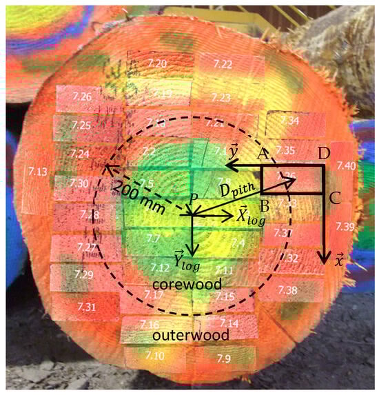
Figure 2.
Photomontage of the painted butt end of a log (log number 7 displayed) with the cross-sections of the 40 × 100 mm2 sawn boards superposed on it. Board No. 7.36 is framed in black as an example to show its local coordinate system (D, ,) and how was obtained. Points A, B, C, and D represent the four corners of the board cross-section. The first fifteen growth rings closest to the pith were painted in green for reference. The dashed circle represents the boundary between corewood and outerwood. For a board to be classified as corewood, its entire cross-section must fit within this circle. For example, board No. 7.36 was considered to be outerwood, whereas board No. 7.7 was considered to be corewood.
is examined in this work as a predictor variable for bending strength IPs.
Ring numbers were counted on the same images of the butt ends of the logs (as in Figure 2), and the average cambial age of each board was determined by averaging the lowest and highest ring numbers observable in the board’s cross-section.
Each board was classified as a corewood board or an outerwood board according to whether its entire cross-section was contained within a 200 mm radius of the pith or not. This classification method was chosen to correspond to boards obtained from logs with a diameter of 400 mm, a common size for canter sawmill lines. As shown in Figure 2, this results in selecting boards that contain a significant portion of corewood, specifically the first fifteen growth rings from the pith (painted in green in this example). It should be noted that boards that we defined as corewood can include some proportions of what can be anatomically defined as mature wood. This classification allows marking the difference between corewood boards, typically obtained from a canter sawmill line, and outerwood boards, which can be produced using a sawmill line capable of processing larger diameter logs (e.g., with a bandsaw). Finally, the sample was divided into 2 groups of similar size, giving 130 outerwood boards and 111 corewood boards.
2.3.3. Knot-Related Parameters
Local density measurements allowed the knot depth ratio (KDR) to be calculated. This value represents the local knot thickness divided by the thickness of the board [30]. The computation of the KDR relied on the fact that knot density is higher than clear wood density. The KDR is equal to 0 in clear wood and 1 when at a given position the thickness of the board is composed entirely of knot. The KDR was calculated using Equation (13), where and are, respectively, the clear wood and knot density, represents the clear wood density variability within a board (), and is the ratio between and :
In order to determine the parameters (,,, and ) a first image processing step was used to separate knotty regions from clear wood regions (based on a Sobel filter [31]). Two examples of the KDR maps obtained for different boards are presented in Figure 3b. They show how high-density latewood, particularly in a quarter-sawn board, was problematic in the KDR computation. For this reason, another processing step was carried out to filter out this remaining artifact. Regions where the KDR gradient in the y-direction was above a given threshold (defined empirically) were simply removed. Lastly, remaining knot regions that were smaller than 50 mm2 were also removed from the analysis. The filtered KDR maps obtained using these last two steps are shown in Figure 3c. The results of this image processing procedure were checked manually, board by board, and only 13 boards still presented false knot regions that were manually removed. This method also allowed the number of knots on each board, denoted , to be counted; they were counted preliminarily using algorithms and then recounted manually to adjust the results when necessary.
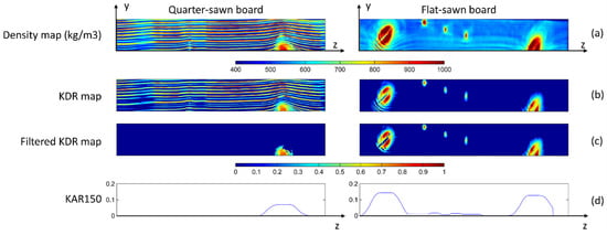
Figure 3.
Examples of KDR and KVR150 calculated for two different boards (only 1-m-long portions shown). (a) Two-dimensional maps of local density obtained by X-ray scanning; (b) initial KDR maps computed using Equation (13); (c) filtered KDR maps; (d) KVR150 computed from the KDR as in Equation (16).
Based on the KDR and the detection of each knot, it was possible to compute the volume of each knot of a board as follows:
where is the region detected as a knot in the 2-dimensional map for the th knot of the board, is the thickness of the board, and = 0.133 mm and = 1 mm are the pixel resolutions. The knot volume ratio within a board (KVRboard) was then computed by summing the knot volumes of a board divided by the volume of this board as follows:
The knot area ratio (KAR) is defined in the literature as the maximum sum of the projected knot areas along the board, located within a 150 mm-long sliding window [32]. Without knowledge of the position of the knots in the thickness direction of the boards, it was not possible to project the knots onto the cross-section, making it impossible to truly compute the KAR within a window. However, it was possible to compute a KAR-like parameter by summing the KDRs along a 150-mm-long moving window, which gave a knot volume ratio within this window, denoted KVR150. Examples of obtained KVR150 profiles are given in Figure 3d. A single KVR150 value was attributed to each board by searching for its maximum in the maximum moment zone between the point loads, so the KVR150 was finally calculated as follows:
where and , respectively, are the positions where the two-point loads were applied in the four-point bending test, i.e., − = 6 h, is the longitudinal position on the board in mm, and is the width of the board. With this definition, the KVR150 value attributed to each board did not necessarily correspond to the weakest part of the entire board, but to the weakest part in the maximum moment zone in the bending test, where the failure occurred. This enabled a fair comparison of KVR150 to the bending strength, which is allowed for the determination of machine settings. However, in actual grading, the most unfavorable value of the knot measure along the entire board should be considered.
2.3.4. Fiber Orientation-Based Predictor Variable
The model used in this study to determine a predictor variable related to fiber orientation was initially proposed by Olsson et al. [14]. It is briefly explained below, and a more detailed description is given in several other studies [14,16,21].
Using this model, it was assumed that the orthotropic elastic properties proposed by Guitard [33], given in Table 3, were valid for the wood material. The same nominal wood properties were used for all the boards and for the entire volume of each board, but the determined local fiber orientation was used to compute, by transformation of the material stiffness matrix, a MoE valid in the longitudinal board direction (). Regarding fiber orientation in the interior of the board, it was assumed that the fiber orientations determined on the four sides of each board were valid to a certain depth into the board. Then, integration over the cross-section of the board was performed, in the way described by Olsson et al. [14], to obtain an MoE valid for bending at each local cross-section along the board. The obtained one-dimensional representation of the bending MoE along the board, with a resolution of 1 mm, was denoted . This MoE profile was smoothed by a moving average along a length of 90 mm, and the minimum value of this profile between the positions where the two-point loads were applied in the four-point bending test was denoted (same notation as used by Olsson et al. [16]). It was used as a predictor variable for strength in this study. The formula to compute this predictor variable can be written as follows:
where and , respectively, are the positions where the two-point loads were applied in the four-point bending test, i.e., − = 6 h, is the longitudinal position in the board in mm, and = 1 mm.
Table 3.
Nominal wood material parameters: E, G, and v are MoEs, shear moduli, and Poisson’s ratios, respectively, and indices l, r, and t refer to the longitudinal, radial, and tangential directions, respectively [30].
2.3.5. Indicating Properties
Among the three GDPs, bending strength is both the most challenging and the most important to predict [15,34]; therefore, this study focused on this GDP. However, the two other GDPs were considered in the grading procedure as well. The IP for density was , i.e., the same property as regarded as the grade-determining density, which corresponds to the assumption that this property can be perfectly determined. The IP used for the grade-determining MoE () was the dynamic modulus of elasticity, .
Several different IPs were tested to predict the grade-determining strength (). They are all listed in Table 4. First, the bending strength itself, , was tested in order to have a reference for the grading yield obtained with a “perfect grading machine.” Secondly, KVR150, , , and were used to get IPs obtained from a single predictor variable. Then, the four possible combinations of the three latter predictor variables were evaluated using multiple linear regression to produce new IPs. For example, a combination involving three of the predictor variables can be expressed as follows:
where , , and are the coefficients that gave the highest possible coefficient of determination between and in the sample and is the value that makes the line of regression go through the origin. Similar equations were obtained for the cases of one and two predictor variables. The IPs obtained this way were in the same unit size as , and the root mean square error for each IP was computed as follows:
where is the number of boards successfully tested, —the grade-determining strength of board i, and —the value of the IPs considered (one of those defined in Table 4) for board i.
Table 4.
Notations and predictor variables of IPs defined using multiple linear regression.
2.3.6. Grading Procedure
The grading procedure is standardized by the rules given in EN 14081-2+A1 [13]. The sampling of this study did not fulfill the requirements of the standard, in terms of representativeness of the resource, and number of boards (at least 450 boards would be required). Therefore, a simplified grading procedure was used.
First of all, no multiple classes were considered in the grading; the boards were simply graded to a given class of EN 338 [35] or rejected. The grading procedure was as follows: (1) the IPs for strength prediction were sorted in a vector by decreasing order; (2) the IP limit between the rejected boards and the boards graded into the class, which is called the IP setting, was set so that no more than 5% of the actual strength values of the boards above the IP setting were below the required characteristic strength of the class; (3) it was verified whether the selected boards fulfilled the criteria for the other GDPs, i.e., if the average of the grade-determining MoEs ( for the set of boards to be assigned to the class exceeded the required average MoE of the class and if the 5% fractile of the grade-determining density exceeded the required characteristic density; (4) if not, a new loop would have been performed, decreasing the number of boards assigned to the class until all requirements were fulfilled (this latter step never happened in practice in this study).
This grading procedure was performed for three different strength classes, namely C24, C30, and C35. The corresponding required characteristic strengths for these classes are 21.4 MPa, 26.8 MPa, and 35 MPa, respectively. Indeed, within the framework of machine grading, EN 14081-2+A1 [13] can allow the division of the characteristic bending strength of the classes under C30 (included) by a factor 1.12. The yield for each class was computed by simply dividing the number of boards graded into the class by the total number of boards. The IP setting was determined for the whole set of boards, and each board was assigned to a class. Thus, it was possible to count the number of outerwood and corewood boards assigned to the class and compute yields for outerwood and corewood boards separately.
Finally, it should be noted that since local predictor variables KVR150 and used in the simulated grading procedure were calculated only with respect to the part of each board placed between the point loads in the bending test, and not the entire board, the yields presented below were higher than what they would have been if the entire length of the board were considered. Still, the yields presented enabled a comparison of the quality of corewood vs. outerwood as well as a comparison of the performance of different IPs.
3. Results
3.1. Comparison of GDPs and Knottiness Parameters Between Corewood and Outerwood
In Table 5, the calculated average values and standard deviations of the GDPs (board density, global MoE, and bending strength) and knottiness parameters (nK, KVRboard, KVR150) are presented for the boards that failed between the loading heads. Thus, from the 241 boards of the initial sample, the results for 221 boards were used. The numbers of outerwood and corewood boards were reduced from 130 to 114, and from 111 to 107, respectively.
Table 5.
Statistical information about the successfully mechanically tested boards for the entire sample and for outerwood (boards located 200 mm to the pith) and corewood (boards located < 200 mm to the pith). Mean values and coefficients of variation (the latter given in parentheses) are given. Student’s t-test was performed to test the difference between the averages of outerwood and corewood. Significant differences are indicated with asterisks (* p < 0.05, *** p < 0.001).
Student’s t-test was performed to compare the means of corewood and outerwood. Despite the sometimes high standard deviations, there were significant differences between all the studied parameters (p < 0.001 for all but the KVR150 parameter, with p = 0.01). GDPs of outerwood systematically outperform those of corewood. Indeed, the mean density, global MoE, and bending strength were, respectively, 7%, 25%, and 31% lower for corewood than for outerwood. There were also clearly many more knots in corewood than in outerwood (8.6 vs. 3.5 as the average number of knots per board within the tested range, respectively), and a higher KVRboard (0.47% vs. 0.22%, respectively). KVR150 was also higher for corewood than for outerwood, but the difference was smaller than for nK and KVRboard (+40% compared to +144% and +108%, respectively).
When considering all the boards, the knottiness parameters presented a higher CoV (66%, 78%, and 99% for nK, KVRboard, and KVR150, respectively) than those of the GDPs (e.g., 44% for , which was the highest CoV of a GDP). Moreover, when considering the difference between corewood and outerwood, it appeared that the CoV of the knottiness parameters was lower for corewood than for outerwood, while it was almost the same for the GDPs.
3.2. Relationships Between GDPs, Dynamic MoE, Cambial Age, Distance to the Pith, and Knottiness
Figure 4 shows that the distance from the center of a board’s cross-section to the pith is linearly correlated to the average cambial age observed within the board’s cross-section. Through the linear regression with the intercept forced to zero, the average annual ring width was determined to be 7.2 mm. The coefficient of determination was 0.99 with a forced intercept and 0.91 without a forced intercept. This result implies that either the distance to the pith or the cambial age would provide similar performance as predictor variables for mechanical properties. Distance to the pith was chosen instead of cambial age because it is easier for a sawmill owner to handle. It can allow them to directly link the study’s results to the log diameter (assuming their supply corresponds to the fast-grown Douglas fir in this study). Additionally, emerging technologies can automatically determine the distance to the pith of a board [23,24,25].
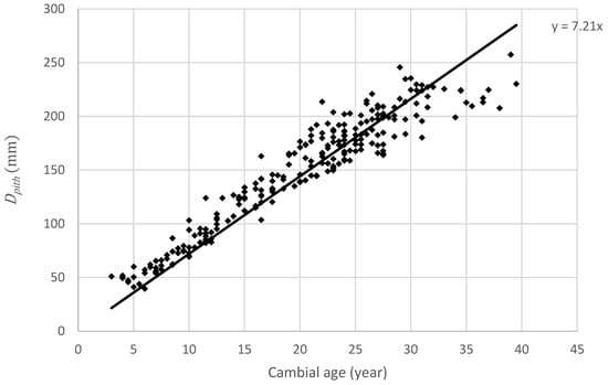
Figure 4.
Distance from the center of a board’s cross-section to the pith of the log according to the average cambial age observed within the board’s cross-section, with a linear regression with the intercept fixed at the origin.
Table 6 shows the coefficients of determination between the distance to the pith, KVRboard, KVR150, the corrected dynamic MoE, , the corrected local MoE, and the three GDPs. It gives the coefficients of determination between each parameter, with the significance level and 95% confidence interval.
Table 6.
Coefficients of determination with confidence intervals. Values in square brackets indicate the 95% confidence interval for each correlation. The confidence interval is a plausible range of population correlations that could have caused the sample correlation. Note: * indicates p < 0.05, ** indicates p < 0.01.
The distance to the pith was positively correlated with the mechanical properties (R2 = 0.25 with and R2 = 0.20 with ) and negatively correlated with the knottiness parameters, especially KVRboard (R2 = 0.22). It was less correlated with (R2 = 0.09) and KVR150 (R2 = 0.03) than with the other parameters.
The best correlation with for a nondestructive predictor variable was obtained for (R2 = 0.88). Board density was the second-best predictor (R2 = 0.57), and was the third (R2 = 0.50).
The corrected local MoE, , was correlated with the strength with R2 = 0.68, and the best correlation with for a nondestructive predictor was obtained for (R2 = 0.61). The second-best correlation with was obtained for (R2 = 0.54). The other parameters presented weaker correlations. KVRboard, which concerned the whole board, presented the same correlation with as KVR150 (based on the part of the board placed between the loading heads), namely 0.34.
3.3. Prediction of Bending Strength by IPs
The results of the prediction of by the different IPs are summarized in Figure 5 for the whole set of boards and for corewood and outerwood separately. Both the RMSE of the prediction of by the different IPs and the coefficients of determination (R2 values) for the whole set of boards are given in the figure.
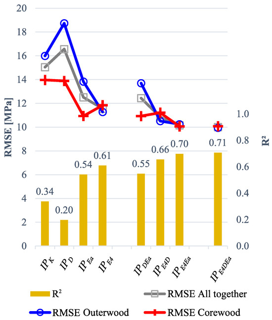
Figure 5.
RMSE and R2 values for the predictions of using the different evaluated IPs.
For the whole set of boards, it appears that the highest RMSE and lowest coefficient of determination (worst prediction) were obtained with as a predictor, i.e., using (RMSE = 16.6 MPa, R2 = 0.20), while and gave a lower RMSE and a higher R2 (12.5 and 11.6 MPa, and R2 = 0.54 and 0.61, respectively). The IP based on KVR150, , showed a higher RMSE than and . Combining and did not result in any significant improvement of the RMSE ( RMSE was 12.4 MPa, R2 = 0.55). However, and allowed for obtaining the RMSE of 10.9 MPa and 10.2 MPa, respectively (R2 = 0.66 and 0.70), instead of 11.5 MPa for only. Combining the three predictors did not significantly improve the RMSE (10.0 MPa, R2 = 0.71).
The results also showed that the RMSEs of the prediction of by , , or were lower for outerwood than for corewood. There was no such difference when using or any of the other IPs, of which is one of the predictors involved (, , ).
3.4. Yields According to IPs and Distance to the Pith
The yields obtained by means of the grading process defined in the Materials and Methods section are presented in Table 7 for three different strength classes: C24, C30, and C35. The yields are given for the 8 IPs previously described plus the bending strength itself in order to show the results that could have been obtained by a perfect machine.
Table 7.
Grading results obtained for the different IPs for classes C24, C30, and C35. For each pair of class and IP, the IP setting is provided is valid for the complete set of boards as well as for outerwood boards and corewood boards separately. The yield is defined as the percentage of boards of each group assigned to a class. The colors associated with the cases are formatted in shades of gray relative to the yield value, with darker shades indicating higher yields and lighter shades indicating lower yields.
The bending strength was the limiting GDP in all cases; thus, the results focused on this property. The IP setting for the bending strength is given in Table 7 for each class and IP. The IP settings are also indicated in Figure 6 (except for ) by vertical dashed lines. The required characteristic strengths are also indicated by horizontal dashed lines. Figure 6 also shows the difference between corewood and outerwood boards, with different marks used in the scatter plots.
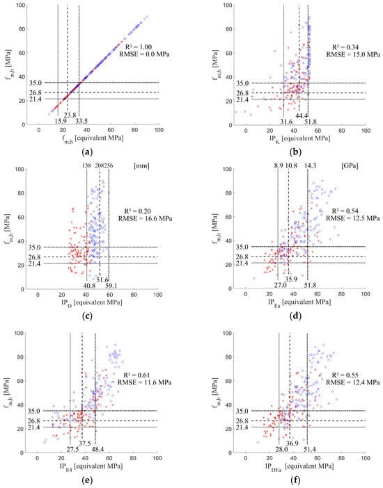
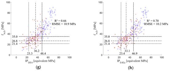
Figure 6.
Scatter plots of in relation to each of the IPs of Table 4 from to (a–h). Red cross marks represent corewood boards and blue circle marks represent outerwood boards. Horizontal lines mark the required characteristic strengths of class C24 (dotted line), C30 (dashed line), and C35 (dash-dotted line). Vertical lines represent the IP settings, meaning that at least 95% of the marks to the right of each line represent boards with the predicted strength exceeding the characteristic strength of the class.
It is worth noting that only 11 boards were below the required C18 characteristic strength of 16.1 MPa, which is 4.98% of the whole set of 221 boards. This means that the whole set of boards would have been graded as C18. In this case, a particular method according to EN 14081-2+A1 [13] should be applied to determine the IP setting, requiring at least 5 boards to be rejected. However, this is not applied here.
The IP settings obtained for the “perfect machine” based on itself were lower than the required characteristic strengths. This was due to the fact that the grading process allows 5% of the boards assigned to a class to be below the required characteristic strength. For the “perfect machine” based on itself, 95% of all the boards were graded as C24, 86% were graded as C30, and 59% were graded as C35. Large differences were observed in Table 7 regarding the yields of C30 and C35 because the corresponding required characteristic strengths for these classes differ significantly (26.8 MPa and 35 MPa, respectively) due to the 1.12 coefficient applied to the required characteristic strength for classes up to C30, as explained in the Materials and Methods section. IP , which is based on three different predictors, generally provided the best results for all the classes, with yields of 89%, 68%, and 46% in C24, C30, and C35, respectively.
For the “perfect machine” based on , there was a higher number of outerwood boards than corewood boards graded in each class. Thus, yields were higher for outerwood boards and lower for corewood boards compared to when considering the whole set of boards. Moreover, the higher the class, the bigger the difference between the outerwood and corewood yields was. For example, in class C35, the yield was 75% for outerwood and only 41% for corewood, while there was only a 3 percentage point difference for class C24 (96% and 93% yield for outerwood and corewood, respectively). All the tested IPs also provided better yields for outerwood than for corewood. However, the differences between the outerwood and corewood yields were larger than for the “perfect machine.” For example, in C30, gave a yield for outerwood of 79% (93% with the “perfect machine”), but for corewood, the yield was only 48% (79% with the “perfect machine”). The same comparison for gave yields of 81% and 58%, for outerwood and corewood, respectively.
In relation to what can be observed in Figure 6, the following comments may be useful to the reader:
- A large number of the outerwood boards were free or almost free of knots in the considered part of the board between the loading heads. As a consequence, for these boards, predictor KVR150 ≈ 0%. This is shown in Figure 6c by several boards/marks clustered at almost the same predicted strength (horizontal axis) just above 50 MPa. One can also notice that some values of were very low due to large knots, sometimes even with negative values appearing because of the linear regression used to compute from high KVR150 values.
- The two populations of corewood and outerwood boards are clearly separated in Figure 6c, which is natural since outerwood boards by definition have a larger distance to the pith than corewood boards. Using for prediction of the pith distance, all outerwood boards were above the C24 IP setting. The strength values of the four very weak outerwood boards (all below 12 MPa) were overestimated, but this number of boards complied with the grading rule (more than 95% of the actual strength values of the boards above the IP setting were above the required characteristic strength of the class).
- The lowest values (below the C24 IP setting) in Figure 6d were almost all from corewood, which naturally presents low axial dynamic MoE values. In contrast to this, the lowest values in Figure 6e represent a mixture of outerwood and corewood boards, as is the case for (Figure 6b). For example, for the boards with an actual bending strength below 35 MPa, the average was 30.9 MPa for corewood and 34.8 MPa for outerwood, while for , it was 33.0 MPa for corewood and 26.0 MPa for outerwood. Hence, when using instead of , the predicted strength of the weakest outerwood boards relative to the weakest corewood boards was lower.
4. Discussion
The discussion below is aimed to compare wood that large industrial sawmills prefer to use (40 cm logs) to what can be obtained with larger logs of 50–55 cm diameter. Since similar numbers of successfully tested outerwood and corewood boards (114 and 107, respectively) were included in the materials, the comparisons between the averages, standard deviations, and grading of these two populations could be made with some confidence. However, this discussion falls under the scope of the resource used, which consisted of fast-grown Douglas fir logs which exhibited an average growth ring width of 7.2 mm, and potentially other environmental parameters that were not taken into account.
4.1. Differences Between the Mechanical Properties of Corewood and Outerwood: Highlights and Interpretations
The mean values of the GDPs that were obtained in this work were comparable to what has been presented in other studies of Douglas fir timber of the same size [12,15,34]. For example, in [15], the average bending strength was 34.1 MPa, which was the same as the average corewood bending strength in this study, consistent with the fact that smaller logs were used (mean diameter at breast height of 43 cm [36]). The coefficient of variation was slightly lower in [15], namely 34%, versus 40% in this work. However, in [37], lower mechanical properties were obtained both for corewood and outerwood of the Douglas fir grown in the UK. Overall, comparisons with results presented in the literature tend to indicate that, despite their small number, the logs used in this work can be rather representative of the natural variability of the properties of the Douglas fir grown in France.
The results showing that the stiffness and strength of corewood timber were, respectively, 25% and 31% lower than those of outerwood match corresponding results presented in the literature. In [22], the MoE of what the authors called juvenile timber, which corresponded to boards containing 1 to 18 rings from the pith, was 50–79% of that of the mature timber obtained from 75-year-old Douglas fir trees, and the modulus of rupture of the juvenile timber was 59–69% of that of the mature timber. In [37], inner boards (boards containing the pith) of Douglas fir logs had a 36% lower strength and a 35% lower MoE than outer boards (boards with a distance to the pith of about 96 mm). Kliger et al. [5] studied fast-grown Norway spruces (Picea abies) of 36 cm diameter at breast height and made a distinction between corewood and outerwood boards. They obtained an 18% lower MoE and a 26% lower strength for corewood compared to outerwood. Thus, the results presented herein are typical not only of Douglas fir, but similar relationships also exist for other softwood species.
In all the previously cited studies on structural timber size [5,22,37], the relative difference of density between corewood and outerwood (or juvenile and mature wood, depending on the terminology used by the authors) was much smaller than that of the mechanical properties, which is consistent with the results of this study (corewood density being only 7% lower than outerwood density). These results may suggest that density is not the main explanatory variable for the difference between corewood and outerwood timber’s mechanical properties. The cellulose orientation in the S2 layer, which varies according to the distance to the pith, is usually assumed to be the principal predictor of timber quality in the literature [2,12,38], even if density also positively correlates with mechanical properties.
Our results highlight the much higher knottiness of corewood compared to outerwood (more than twice the number and twice the volume of knots per board in corewood). Having more knots in the corewood was expected, but it was not obvious from the outset that KVRboard would be higher in the corewood, since knots in the corewood are smaller. Only a few quantitative studies on the occurrence of knots in corewood and outerwood are presented in the literature. Kliger et al. [5], who investigated the same material as in [4], found similar results to those presented herein by comparing the KAR between corewood and outerwood of fast-grown Norway spruce (Picea abies) and reported values of 0.31 and 0.22, respectively. In our results, the variation in knottiness parameters was also much higher for outerwood than for corewood. Of course, this is not very surprising since knots in outerwood are few but large. In most sections along outerwood boards, there are no knots, but if a large knot passes through the center of the board, any local knot measure used would show a large value. Similar results were presented in [4] and explained in the same way.
Corewood having more knots in both number and volume ratio, it was not surprising to obtain a lower MoE in the corewood than in the outerwood, knots being weak zones and causing grain deviation. Interestingly, the weakest cross-section of the corewood boards also presented higher KVR150 values (40% higher for the corewood compared to the outerwood). These results suggest that the higher knottiness of corewood should be a major reason for both its lower MoE and bending strength, which is rarely highlighted in the literature, which authors usually search for the explanation only in the juvenile nature of wood fibers (i.e., the cellulose microfibril angle in the S2 layer).
4.2. Potential Benefits of Knowing the Board Distance to the Pith for Strength Grading
The distance to the pith presented the lowest coefficient of determination to of all the IPs considered in this research. However, since the distance to the pith is correlated with the number and size of knots and the microfibril angle of wood fibers, we aimed to test whether it could be useful for grading.
Using the distance to the pith alone as an IP allowed grading all the outerwood boards into the C24 class. Indeed, the outerwood had rather high mechanical properties, and in particular, more than 95% of the outerwood boards were above the required characteristic bending strength of the C24 class. Thus, the IP setting corresponding to the C24 class was a distance to the pith of 138 mm (Figure 6c), which means from a practical point of view that if a machine, such as one based on a camera shooting at the butt end of the logs, would be able to provide the information whether a portion of a 40 × 100 mm2 board was above a 138 mm of distance to the pith, it could grade this board into the C24 class. This, however, may not be of practical interest for machine grading, because it would imply that all the boards strictly below this limit would be rejected, leading to a rather poor overall yield of 62%. It could also work only for the C24 class, the yields in other classes being considerably lower. Moreover, another existing machine, such as one based on dynamic MoE, would be able to perform better overall, correctly grading corewood. However, in the context of visual grading, knowing whether a board is above this limit may be useful, just as Kennedy suggested [11].
When used in combination with a predictor variable such as helps to raise the coefficient of determination to (from 0.61 using to 0.66 using and increase yields in strength classes. This makes perfect sense, as the two predictor variables complement each other. captures the occurrence of fiber distortions and knots in detail, but does not contain any information on the quality of wood fibers (microfibril angle in the S2 layer and density), which does, since the quality of the fibers changes with the distance to the pith. However, using in combination with , an even higher coefficient of determination is obtained (0.70 using ,), and yields in strength classes become even higher as well. Unfortunately, the combined use of all three predictor variables does not result in any significant further improvement (a coefficient of determination of 0.71 obtained using ). From a practical point of view, if a scanner is used to determine both the local fiber direction on board surfaces and the location of the pith, it may be of interest to use instead of (i.e., instead of ), since then no device for the dynamic excitation of boards would be needed. However, this result should be confirmed with a larger study including trees subjected to different forest management strategies: indeed, thinning can have a significant influence on the diameter and mechanical properties of timber [39]; thus, the effect of the distance to the pith may be different depending on the forest management strategy, which could be taken into account in a model if tracking from the forest to the board is performed.
5. Conclusions
The main conclusions of this research are as follows:
- (1)
- Corewood boards of large (>500 mm diameter) Douglas fir logs tested in this study had a 31% lower average bending strength and a 25% lower average MoE than outerwood boards.
- (2)
- Corewood boards present a higher knot volume ratio and number of knots than outerwood boards (+40% in the weakest 150-mm-long section), which is a major explanation for their lower mechanical properties in comparison with outerwood boards.
- (3)
- It appears possible to grade all 40 × 100 mm2 boards above a radius of 138 mm into the C24 class without the need to use any other IP than the distance to the pith, which may be of interest for visual grading of Douglas fir.
- (4)
- The distance to the pith does not provide more information for strength prediction than the axial dynamic MoE. As a result, a machine based on a combination of axial dynamic MoE and fiber orientation measurements provides an efficient grading of outerwood boards as well as of corewood boards.
- (5)
- The distance to the pith can be used as part of an IP in combination with a model based on fiber orientation measurement to improve grading efficiency, which may be useful for a machine based on optical measurements only (without vibrational measurements).
Based on the yields obtained for a set of 221 boards, a sawmill processing logs similar to those of this study could achieve yields of up to 70% in the C30 class and 39% in the C35 class by using a grading machine that combines dynamic MoE and fiber orientation measurements. In contrast, a typical industrial sawmill processing logs with diameters mainly below 40 cm (i.e., corewood) would achieve yields of 58% and 10% for the C30 and C35 classes, respectively. However, for the most common C24 class, the yields would be very similar, at 87% and 84%, respectively. These figures indicate a general trend but should be interpreted with caution and confirmed through studies with larger sample sizes. In particular, future research should focus on investigating the impact of reaction wood, position along the stem, growth rate, forest management practices, and other environmental factors to provide a more comprehensive understanding of the relationship between wood morphology and its mechanical properties.
Author Contributions
Funding acquisition, G.P.; writing—original draft preparation, G.P.; writing—review and editing, J.V. and A.O.; data production, G.P., J.V. and A.O.; data analysis, G.P. and A.O.; designing and conducting the experiments, J.V. All authors have read and agreed to the published version of the manuscript.
Funding
This research was funded by the French national research agency, EffiQuAss project, grant number ANR-21-CE10-0002. The authors gratefully acknowledge the support from the Knowledge Foundation through the project “Competitive timber structures—Resource efficiency and climate benefits along the wood value chain through engineering design” (grant number 20230005).
Data Availability Statement
The datasets used and/or analyzed in this study are available from the corresponding author upon reasonable request.
Conflicts of Interest
The authors declare no conflicts of interest. The funders had no role in the design of the study; in the collection, analyses, or interpretation of data; in the writing of the manuscript; or in the decision to publish the results.
References
- Zobel, P.D.B.J.; Sprague, J.R. Juvenile Wood in Forest Trees; Springer: Berlin/Heidelberg, Germany, 1998. [Google Scholar]
- Lachenbruch, B.; Moore, J.R.; Evans, R. Radial Variation in Wood Structure and Function in Woody Plants, and Hypotheses for Its Occurrence. In Size- and Age-Related Changes in Tree Structure and Function; Meinzer, F.C., Lachenbruch, B., Dawson, T.E., Eds.; Springer: Dordrecht, The Netherlands, 2011; pp. 121–164. [Google Scholar]
- Pollet, C.; Henin, J.-M.; Hébert, J.; Jourez, B. Effect of growth rate on the physical and mechanical properties of Douglas-fir in western Europe. Can. J. For. Res. 2017, 47, 1056–1065. [Google Scholar] [CrossRef]
- Perstorper, M.; Pellicane, P.J.; Kliger, I.R.; Johansson, G. Quality of timber products from Norway spruce. Wood Sci. Technol. 1995, 29, 157–170. [Google Scholar] [CrossRef]
- Kliger, I.R.; Perstorper, M.; Johansson, G. Bending properties of Norway spruce timber. Comparison between fast- and slow-grown stands and influence of radial position of sawn timber. Ann. For. Sci. 1998, 55, 349–358. [Google Scholar] [CrossRef]
- Burdon, R.D.; Kibblewhite, R.P.; Walker, J.C.F.; Megraw, R.A.; Evans, R.; Cown, D.J. Juvenile Versus Mature Wood: A New Concept, Orthogonal to Corewood Versus Outerwood, with Special Reference to Pinus radiata and P. taeda. For. Sci. 2004, 50, 399–415. [Google Scholar] [CrossRef]
- Mora, C.R.; Allen, H.L.; Daniels, R.F.; Clark, A. Modeling Corewood–Outerwood Transition in Loblolly Pine Using Wood Specific Gravity. Can. J. For. Res. 2007, 37, 999–1011. [Google Scholar] [CrossRef]
- Moore, J.R.; Cown, D.J. Corewood (Juvenile Wood) and Its Impact on Wood Utilisation. Curr. For. Rep. 2017, 3, 107–118. [Google Scholar] [CrossRef]
- Clark, A.; Saucier, J.R. Influence of Initial Planting Density, Geographic Location, and Species on Juvenile Wood Formation in Southern Pine. For. Prod. J. 1989, 39, 42–48. [Google Scholar]
- Gapare, W.J.; Wu, H.X.; Abarquez, A. Genetic Control of the Time of Transition from Juvenile to Mature Wood in Pinus Radiata D. Don. Ann. For. Sci. 2006, 63, 871–878. [Google Scholar] [CrossRef]
- Kennedy, R.W. Coniferous wood quality in the future: Concerns and strategies. Wood Sci. Technol. 1995, 29, 321–338. [Google Scholar] [CrossRef]
- Rais, A.; Poschenrieder, W.; Pretzsch, H.; van de Kuilen, J.-W.G. Influence of initial plant density on sawn timber properties for Douglas-fir (Pseudotsuga menziesii (Mirb.) Franco). Ann. For. Sci. 2014, 71, 617–626. [Google Scholar] [CrossRef]
- EN 14081-2+A1; Timber Structures—Strength Graded Structural Timber with Rectangular Cross Section—Part 2: Machine Grading; Additional Requirements for Type Testing. European Committee for Standardization: Brussels, Belgium, 2022.
- Olsson, A.; Oscarsson, J.; Serrano, E.; Källsner, B.; Johansson, M.; Enquist, B. Prediction of timber bending strength and in-member cross-sectional stiffness variation on the basis of local wood fibre orientation. Eur. J. Wood Wood Prod. 2013, 71, 319–333. [Google Scholar] [CrossRef]
- Viguier, J.; Bourreau, D.; Bocquet, J.-F.; Pot, G.; Bléron, L.; Lanvin, J.-D. Modelling mechanical properties of spruce and Douglas fir timber by means of X-ray and grain angle measurements for strength grading purpose. Eur. J. Wood Wood Prod. 2017, 75, 527–541. [Google Scholar] [CrossRef]
- Olsson, A.; Pot, G.; Viguier, J.; Faydi, Y.; Oscarsson, J. Performance of Strength Grading Methods Based on Fibre Orientation and Axial Resonance Frequency Applied to Norway Spruce (Picea abies L.), Douglas Fir (Pseudotsuga menziesii (Mirb.) Franco) and European Oak (Quercus petraea (Matt.) Liebl./Quercus robur L.). Ann. For. Sci. 2018, 75, 102. [Google Scholar] [CrossRef]
- Rais, A.; Bacher, M.; Khaloian-Sarnaghi, A.; Zeilhofer, M.; Kovryga, A.; Fontanini, F.; Hilmers, T.; Westermayr, M.; Jacobs, M.; Pretzsch, H.; et al. Local 3D Fibre Orientation for Tensile Strength Prediction of European Beech Timber. Constr. Build. Mater. 2021, 279, 122527. [Google Scholar] [CrossRef]
- Lukacevic, M.; Kandler, G.; Hu, M.; Olsson, A.; Füssl, J. A 3D model for knots and related fiber deviations in sawn timber for prediction of mechanical properties of boards. Mater. Des. 2019, 166, 107617. [Google Scholar] [CrossRef]
- Olsson, A.; Pot, G.; Viguier, J.; Hu, M.; Oscarsson, J. Performance of Timber Board Models for Prediction of Local Bending Stiffness and Strength—With Application on Douglas Fir Sawn Timber. Wood Fiber Sci. 2022, 54, 226–245. [Google Scholar] [CrossRef]
- Huber, J.A.J.; Broman, O.; Ekevad, M.; Oja, J.; Hansson, L. A Method for Generating Finite Element Models of Wood Boards from X-Ray Computed Tomography Scans. Comput. Struct. 2022, 260, 106702. [Google Scholar] [CrossRef]
- Pot, G.; Duriot, R.; Girardon, S.; Viguier, J.; Denaud, L. Comparison of Classical Beam Theory and Finite Element Modelling of Timber from Fibre Orientation Data According to Knot Position and Loading Type. Eur. J. Wood Prod. 2024, 82, 597–617. [Google Scholar] [CrossRef]
- Bendtsen, B.A.; Plantiga, P.; Snellgrove, T.A. The Influence of Juvenile Wood on the Mechanical Properties of 2 x 4 Cut from Douglas-Fir Plantations. In Proceedings of the International Conference on Timber Engineering, Seattle, WA, USA, 19–22 September 1988. [Google Scholar]
- Habite, T.; Abdeljaber, O.; Olsson, A. Determination of Pith Location along Norway Spruce Timber Boards Using One Dimensional Convolutional Neural Networks Trained on Virtual Timber Boards. Constr. Build. Mater. 2022, 329, 127129. [Google Scholar] [CrossRef]
- Abdeljaber, O.; Habite, T.; Olsson, A. Automatic Estimation of Annual Ring Profiles in Norway Spruce Timber Boards Using Optical Scanning and Deep Learning. Comput. Struct. 2023, 275, 106912. [Google Scholar] [CrossRef]
- Li, X.; Pot, G.; Ngo, P.; Viguier, J.; Penvern, H. An Image Processing Method to Recognize Position of Sawn Boards within the Log. Wood Sci. Technol. 2023, 57, 1401–1420. [Google Scholar] [CrossRef]
- Abdeljaber, O.; Olsson, A. Cross-Sectional Analysis of Timber Boards Using Convolutional Long Short-Term Memory Neural Networks. Constr. Build. Mater. 2024, 451, 138855. [Google Scholar] [CrossRef]
- EN 384+A2; Structural Timber—Determination of Characteristic Values of Mechanical Properties and Density. European Committee for Standardization: Brussels, Belgium, 2022.
- EN 408+A1; Timber Structures—Structural Timber and Glued Laminated Timber—Determination of Some Physical and Mechanical Properties. European Committee for Standardization: Brussels, Belgium, 2012.
- The GIMP Development Team. GNU Image Manipulation Program (GIMP), Version 2.8.14. Community, Free Software (license GPLv3). 2014. Available online: https://www.gimp.org/about/linking.html (accessed on 8 March 2025).
- Oh, J.-K.; Shim, K.; Kim, K.-M.; Lee, J.-J. Quantification of knots in dimension lumber using a single-pass X-ray radiation. J. Wood Sci. 2009, 55, 264–272. [Google Scholar] [CrossRef]
- Kanopoulos, N.; Vasanthavada, N.; Baker, R.L. Design of an image edge detection filter using the Sobel operator. IEEE J. Solid-State Circuits 1988, 23, 358–367. [Google Scholar] [CrossRef]
- Roblot, G.; Bleron, L.; Meriaudeau, F.; Marchal, R. Automatic Computation of the knot area ratio for machine strength grading of Douglas-fir (Pseudotsuga menziesii) and Spruce (Picea excelsa) timber. Eur. J. Environ. Civ. Eng. 2010, 14, 1317–1332. [Google Scholar] [CrossRef]
- Guitard, D. Mécanique du Matériau Bois et Composites; Cépaduès: Paris, France, 1987. [Google Scholar]
- Gil-Moreno, D.; Ridley-Ellis, D.; Harte, A.M. Timber grading potential of Douglas fir in the Republic of Ireland and the UK. Int. Wood Prod. J. 2019, 10, 64–69. [Google Scholar] [CrossRef]
- EN 338:2016; Structural Timber—Strength Classes. European Committee for Standardization: Brussels, Belgium, 2016.
- Viguier, J. Strength Grading of Structural Timber. Consideration of Local Singularities to Predict Mechanical Properties. Ph.D. Thesis, Université de Lorraine, Epinal, France, 2015. [Google Scholar]
- Drewett, T.A. The Growth and Quality of UK-Grown Douglas-Fir. Ph.D. Thesis, Edinburgh Napier University, Edinburgh, UK, 2015. [Google Scholar]
- Cave, I.D.; Walker, J.C.F. Stiffness of wood in fast-grown plantation softwoods: The influence of microfibril angle. For. Prod. J. 1994, 44, 43–48. [Google Scholar]
- Krajnc, L.; Farrelly, N.; Harte, A.M. The effect of thinning on mechanical properties of Douglas fir, Norway spruce, and Sitka spruce. Ann. For. Sci. 2019, 76, 3. [Google Scholar] [CrossRef]
Disclaimer/Publisher’s Note: The statements, opinions and data contained in all publications are solely those of the individual author(s) and contributor(s) and not of MDPI and/or the editor(s). MDPI and/or the editor(s) disclaim responsibility for any injury to people or property resulting from any ideas, methods, instructions or products referred to in the content. |
© 2025 by the authors. Licensee MDPI, Basel, Switzerland. This article is an open access article distributed under the terms and conditions of the Creative Commons Attribution (CC BY) license (https://creativecommons.org/licenses/by/4.0/).