Forest Canopy Image Segmentation Based on the Parametric Evolutionary Barnacle Optimization Algorithm

Abstract

Forest canopy image is a necessary technical means to obtain canopy parameters, whereas image segmentation is an essential factor that affects the accurate extraction of canopy parameters. To address the limitations of forest canopy image mis-segmentation due to its complex structure, this study proposes a forest canopy image segmentation method based on the parameter evolutionary barnacle optimization algorithm (PEBMO). The PEBMO algorithm utilizes an extensive range of nonlinear incremental penis coefficients better to balance the exploration and exploitation process of the algorithm, dynamically decreasing reproduction coefficients instead of the Hardy-Weinberg law coefficients to improve the exploitation ability; the parent generation of barnacle particles ($pl$ = 0.5) is subjected to the Chebyshev chaotic perturbation to avoid the algorithm from falling into premature maturity. Four types of canopy images were used as segmentation objects. Kapur entropy is the fitness function, and the PEBMO algorithm selects the optimal value threshold. The segmentation performance of each algorithm is comprehensively evaluated by the fitness value, standard deviation, structural similarity index value, peak signal-to-noise ratio value, and feature similarity index value. The PEBMO algorithm outperforms the comparison algorithm by $91.67\%,55.56\%,62.5\%,69.44\%$, and $63.89\%$ for each evaluation metric, respectively. The experimental results show that the PEBMO algorithm can effectively improve the segmentation accuracy and quality of forest canopy images.

1. Introduction

Image segmentation is the process of dividing the pixel points of the original image into different categories of sub-regions according to attributes such as color, texture, and intensity value, and then completing the process of extracting the target in the image [1]. Standard segmentation methods include the thresholding method [2,3,4,5], region technique [6], watershed algorithm [7], and deep learning [8,9,10]. The region-based segmentation method has a severe segmentation deficiency for aggregated particle adhesion [11]. The watershed algorithm has the disadvantage of over-segmentation and reflected light interfering with the image [12]. Deep learning is widely used in forest canopy image segmentation owing to its high segmentation accuracy, robustness, adaptability, and ability to handle large-scale data. U-Net, Mask R-CNN and Transformers are classical segmentation modules in deep learning. However, segmentation methods based on deep learning also suffer from high training cost. They are long and time-consuming, have limitations in being sensitive to noise, and are not suitable for segmenting small-sample images with little feature information and high randomness. Compared to the deep learning method, the threshold segmentation method utilizes the information in the image histogram to find the threshold value of the image. It distinguishes different target and background regions by setting multiple threshold values [13]. Since it relies on simple mathematical operations, it outperforms complex deep learning models in terms of processing speed. The key to threshold segmentation is selecting an appropriate segmentation method to determine the segmentation threshold. Threshold selection methods based on information entropy have attracted considerable attention owing to their clear mathematical concepts. Otsu entropy [14], Renyi entropy [15], and Kapur entropy [16] are typical information entropy methods. The Otsu method selects segmentation thresholds to maximize the variance between the target and background classes. It is suitable for the case where the area occupied by the target and the background in the image are close, and the Otsu segmentation method will be invalid when the area occupied by the two is disparate [17]. The essence of Renyi entropy is to use the subordination function to convert the image histogram information into a fuzzy domain and then obtain the optimal threshold value to segment the image based on the principle of maximum entropy [18]. The adjustable parameter $\alpha$ is an essential parameter in Renyi entropy, and the value of $\alpha$ determines the form of Renyi entropy. Although different segmentation effects can be obtained by adjusting $\alpha$, it is a challenge to select the optimal parameter reasonably. Improper selection may lead to over-segmentation or under-segmentation phenomenon. The segmentation principle of Kapur entropy is that the total entropy value of the target class and the background class is the maximum. Because Kapur entropy is based on the grey level intra-class probability when calculating the entropy value, it is not sensitive to the size of the divided target and background, can better retain small targets in the image [19], and is widely used in color image segmentation.

Forest canopy images have various complex backgrounds, and the gray levels vary widely, requiring multiple thresholds for accurate segmentation. Traditional image segmentation methods use enumeration, and when performing threshold segmentation, each combination must be individually tested to select the optimal threshold. The computational complexity increases exponentially with an increase in the number of thresholds. To overcome these limitations, scholars view finding the optimal thresholds in multithreshold segmentation as an optimization problem with constraints. Heuristic optimization algorithms search for optimal thresholds to reduce the computational complexity. Intelligent optimization algorithms, such as the Golden Jackal Optimization Algorithm [20], Elephant Herding Optimization Algorithm [21], Sand Cat Optimization Algorithm [22], and Dung Beetle Optimization Algorithm [23] have been successfully applied to image segmentation. Studies have shown that the performance of intelligent algorithms significantly affects the segmentation accuracy and efficiency of the images. Therefore, improving intelligent algorithms to enhance their performance and image segmentation accuracy and efficiency has become the focus of research. Sukanta Nama proposes a quasi-reflected slime mold (QRSMA) method combined with a quasi-reflective learning mechanism. The results of the CEC2020 benchmark function tests showed that QRSMA outperformed the statistical, convergence, and diversity measures of the slime mold algorithm. It also outperformed other existing methods for segmenting COVID-19 X-ray images [24]. Jiquan Wang et al. proposed a Whale Optimization Algorithm combining mutation and de-similarity to address the limitations of the whale optimization Algorithm easily falling into local optimal solutions. Multilevel threshold segmentation was performed on ten grayscale images using Kapur and Otsu as the objective function. The experimental results showed that CRWOA outperformed the five compared algorithms in terms of convergence and segmentation quality [25]. Essam H. Houssein et al. proposed a chimpanzee optimization algorithm (IChOA) based on the strategy of contrastive learning and Levy Flight improvement. IChOA was tested on a dataset from the database of infrared images using Otsu and Kapur methods. The experimental results show that the IChOA is robust for segmenting various positive and negative cases [26]. Laith Abualigah et al. proposed a novel hybrid algorithm (MPASSA) to determine the optimal thresholds in multi-threshold segmentation by borrowing the properties of the Marine Predator and Salp Swarm Algorithm. Multiple benchmark images were used to verify the performance of the MPASSA. The experimental results show that MPASSA avoids the problem of falling into the local optima. It also has a strong solution capability for image-segmentation problems [27].

To address the problems of poor segmentation accuracy of forest canopy images due to complex structure and uneven illumination, Wu et al. proposed a segmentation method based on differential evolutionary whale optimization algorithm [28]; Tong et al. proposed a segmentation method based on improved northern goshawk algorithm by using multi-strategy fusion [29]; Wang et al. proposed a segmentation method based on improved tuna swarm optimization [30]. The experimental results show that compared with the original algorithm, the improved algorithm obtains higher segmentation accuracy in segmenting forest canopy images. It proves the effectiveness and necessity of the improved intelligent algorithm in multi-threshold segmentation of forest canopy images. In recent years, scholars have been enthusiastic about innovative algorithms, and many intelligent algorithms with excellent performance have appeared, bringing new vitality to the research on image multi-threshold segmentation. The BMO is a novel bionic evolutionary optimization algorithm proposed by Sulaiman et al. (2018) that simulates the mating behavior of barnacles in nature to solve the optimization problem [31]. Since its proposal, it has received extensive attention from scholars. In [32], quasi-inverse dyadic learning and logistic chaotic mapping were used to solve the problem of the premature convergence of the BMO algorithm. Literature [33] used random wandering was used to replace the random logarithm $rand$ in the remote insemination iteration formula. The parameter p was replaced with a logistic chaotic mapping operator to improve the problem of premature convergence of the BMO algorithm. Literature [34] improved the penis coefficient $pl$ and the remote insemination iterative formula using a logistic model to achieve adaptive transformation of parameters as well as to avoid falling into local optima. In [35], cubic chaos initialization was used to improve the diversity of the initial population, the parameter p was replaced with a hyperbolic sinusoidal modulation factor to improve the convergence speed of the algorithm, and Gaussian and Cosey variants were introduced to solve the shortcomings of the BMO, which is prone to fall into local optimother. The literature [36] integrates barnacle larvae settlement and adhesion behavior to increase population diversity and improve the global exploration performance of the algorithm. It also uses positive and negative decline casting strategies to improve the local mining ability.

The BMO algorithm exhibited an excellent performance and fewer control parameters. However, these parameters have a more significant impact on the performance of the BMO algorithm. Many improvements have also focused on the importance of the parameters of the BMO algorithm, and the direction of its improvement is almost always centered around the parameters. This is explicitly embodied in the following aspects: (1) The fixed penis coefficient makes the exploration and exploitation process unbalanced, although the literature [34] realized the adaptive conversion of $pl$, the range of variation of $pl$ was small, and there was not much difference with the fixed penis coefficient. (2) The Hardy-Weinberg law coefficient p plays a decisive role in the exploitation ability of the BMO algorithm, and fixed coefficients cannot maintain the diversity of the populations, which weakens the exploitation ability of the BMO algorithm. Literature [33] utilized Logistic Chaos coefficients instead of the parameter p. Although Logistic Chaos coefficients have strong ergodicity, their iteration sequences are unevenly distributed, which is not conducive to increasing population diversity. Reference [35] designed a nonlinearly decreasing parameter p in the interval $[0,1]$, which aims to accelerate the convergence speed of the algorithm, but p tends to 0 in the late iteration, which also results in the loss of population diversity. In addition, to improve the ability of the BMO algorithm to jump out of the local optimal solution, ref. [35] added a double perturbation, which effectively enhances the ability of the algorithm to jump out of the local optimal solution but also slows down the convergence speed of the algorithm.

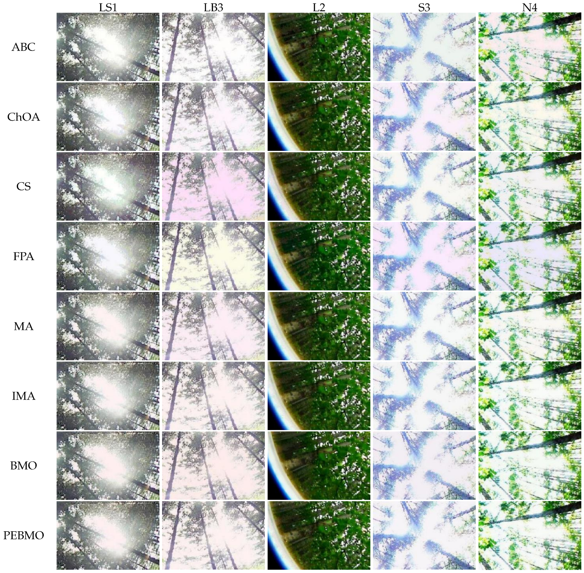
This paper proposes a PEBMO algorithm and applies it to the multi-threshold segmentation of forest canopy images. Specifically, the main contributions of this study are (a) to address the limitations of the BMO algorithm, a wide range of nonlinear increasing penis coefficients, dynamically decreasing reproduction coefficients, and Chebyshev chaotic perturbation strategies are employed to improve the balance between exploration and exploitation, the exploitation ability, and the resistance to premature maturation of the BMO algorithm; (b) the PEBMO algorithm is combined with Kapur entropy to determine the optimal segmentation threshold to improve the segmentation efficiency and accuracy of forest canopy images; and (c) to investigate the performance of PEBMO and PEBMO-based segmentation methods on the 2017 test function and forest canopy image problems, respectively. (d) We compared PEBMO with five BMO variant algorithms. PEBMO performed better than the other BMO-variant algorithms. The forest canopy image segmentation results show that PEBMO-based segmentation methods outperform the artificial bee colony optimization algorithm (ABC) [37], chimp optimization algorithm (ChOA) [38], cuckoo algorithm (CS) [39], flower pollination algorithm (FPA) [40], mayfly algorithm (MA) [41], improved mayfly algorithm (IMA) [42], and BMO.

2. Materials and Methods

2.1. Materials

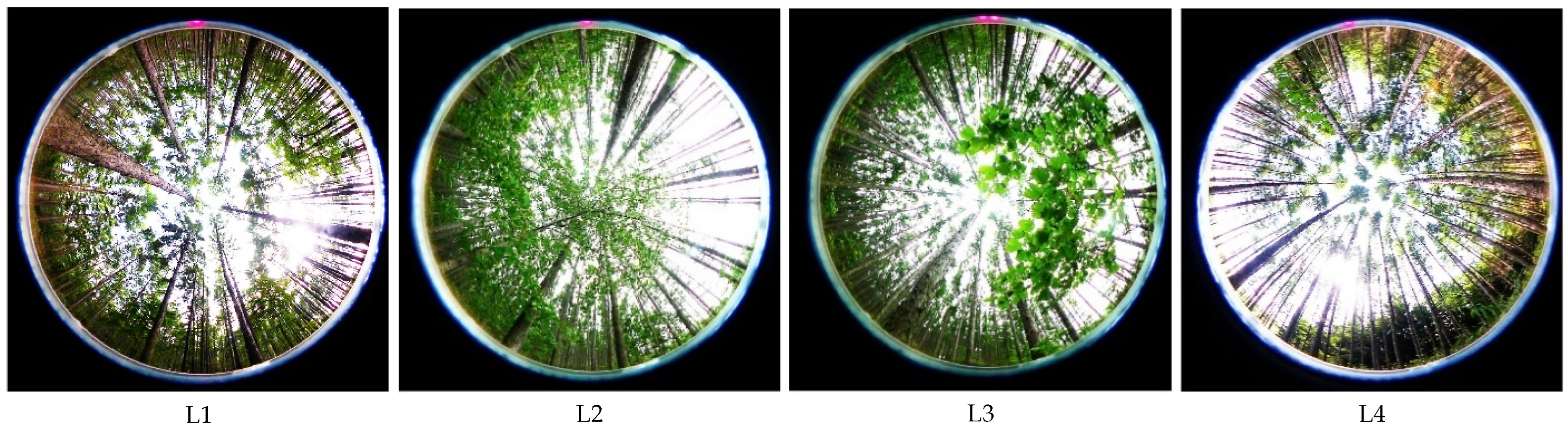
The canopy images used in the experiment were obtained from the Liangshui Experimental Forestry Farm of Northeast Forestry University. They were acquired randomly by a Panasonic DMC-LX5 camera (Panasonic Company, Kadoma City, Osaka, Japan) fisheye lens Samyang AE 8/3.5 Aspherical IF MC Fisheye (Samyang Optics, Changwon, Gyeongsangnam-do, Republic of Korea). The Liangshui Experimental Forest Farm is located in the southern section of the Xiaoxinganling Mountain Range (eastern slope of the Dali Belt Range branch) in the eastern mountains of northeast China. The geographic coordinates are 128°${47}^{\prime }{8}^{″}$–128°${57}^{\prime }{19}^{″}$ E, 47°$6^{\prime }{49}^{″}$–47°${16}^{\prime }{10}^{″}$ N. This location is on the eastern edge of the Eurasia continent, which is deeply influenced by the oceanic climate and has prominent temperate continental monsoon climate characteristics. In winter, under the control of the metamorphic continental air masses, the climate is cold, dry, and windy. In summer, under the influence of subtropical metamorphic oceanic air masses, precipitation is concentrated (of which June–August accounts for more than 60% of annual precipitation), and temperature is high. The climate in spring and fall is variable and spring is windy, with little precipitation, and prone to drought. In the fall, the temperature drops sharply, and early frosts occur more often. The soils in the region are divided into four soil classes (drenching soil class, Semi-hydro pedogenic class, pedogenic class, and organic soil class), four soil classes (dark brown loam, meadow soil, swamp soil, and peat soil), and 14 subclasses. Because the altitude of this area is not high, there is no apparent high mountain, and the vertical distribution of soil is not apparent, only a territorial distribution pattern. Red pine, spruce forests and birch forests dominate in the forest field, accounting for 63.7%, 11.4% and 6.4% of the forested area respectively. The forest cover rate is 98%.

2.2. Basic BMO

Initialization: In the BMO algorithm, barnacles are candidate solutions and the following matrix represents their population vectors:

$$X=\left[\begin{array}{ccc}{X}_1^1& \cdots & X_1^N\\ ⋮& \ddots & ⋮\\ X_n^1& \cdots & X_n^N\end{array}\right]$$

(1)

N is the number of control variables (problem dimensions) and n is the population size or the number of barnacles. The upper-and lower-bound constraints for each control variable are as follows:

$$ub=\left[u{b}_1,\dots ,u{b}_i\right]$$

(2)

$$lb=\left[l{b}_1,\dots ,l{b}_i\right]$$

(3)

where $ub$ and $lb$ denote the upper and lower bounds of the ith variable, respectively. First, the initial population X is evaluated, then the fitness value of each barnacle is ranked, and the barnacle with the best current fitness value is ranked at the top of X.

Selection: Randomly selecting the father and mother to be mated from the barnacle population, the formulae for selection are shown in (4) and (5):

$$x_d=\mathrm{randperm}\left(n\right)$$

(4)

$$x_m=\mathrm{randperm}\left(n\right)$$

(5)

where $x_d$ denotes the father to be mated and $x_m$ denotes the mother to be mated.

Reproduction: The value $pl$ is essential to determine the exploration and exploitation processes. The value $pl$ in the basic BMO algorithm is set to 7. If $pl<7$, the barnacle algorithm reproduces the offspring according to the Hardy-Weinberg theorem, which is the exploitation phase of the BMO algorithm. The barnacle mating iteration formula is given by (6).

$$x_i^{N\_new}=p{x}_d^N+q{x}_m^N$$

(6)

where p and q are the percentages of characteristics of the father and mother in the next generation, respectively. Where p is a random number uniformly distributed in $[0,1]$ and $q=(1-p)$, and are the variables of father and mother selected by Equations (4) and (5), respectively.

If $pl>7$, the offspring are produced by remote insemination, and this process can be considered as an exploration phase with the iterative formula shown in (7):

$$x_i^{n-new}=rand\left(\right)\times x_m^n$$

(7)

where $rand\left(\right)$ is a random number within $[0,1]$, which can be seen from Equation (7) that the mother determines the generation of offspring during remote insemination.

2.3. PEBMO

2.3.1. Large Range of Non-Linear Increasing Penis Coefficients

The penis coefficient $pl$ directly determines the transition between the exploration and exploitation of BMO algorithms. In the basic BMO algorithm, $pl$ is fixed value 7. A fixed penis coefficient defeats the original purpose of the metaheuristic algorithm of dynamic balance between exploration and exploitation. Therefore, it is necessary to design a dynamic adaptive penis coefficient to improve the flexibility between exploration and exploitation. The improved $pl$ parameter is given by Equation (8).

$$plnew=p{l}_1+p{l}_2+p{l}_3$$

(8)

$$p{l}_1=27$$

(9)

$$p{l}_2=-e^{{\left({\displaystyle \frac{T-2t}{T}}\right)}^3}$$

(10)

$$p{l}_3=\tan \left({\displaystyle \frac{t}{T}}\right)$$

(11)

where t is the current number of iterations, and T is the maximum number of iterations.

As can be seen from Equation (8), $plnew$ consists of three parts: $p{l}_1$ is the range adjustment part that determines the overall range of $plnew$. $plnew$ was initially designed to utilize the nonlinearity of $plnew$ to enhance the balance between algorithm exploration and exploitation, and the nonlinearity of the exponential function meets this requirement. The designed $p{l}_2$ increases nonlinearly in the interval [7, 26.95], which makes the $plnew$ value smaller at the beginning of the iteration and gradually increases at the end of the iteration. $p{l}_2$ determines the overall trend of $plnew$ and is the core part of $plnew$. However, $p{l}_2$ gradually reached its maximum value at the end of the iteration and remained there until the end. The $plnew$ that no more changes increases the probability of the algorithm falling into a locally optimal solution. Therefore, it is necessary to make $p{l}_2$ change slightly at the end to enhance the diversity of the population. However, a significant increase is detrimental to the fast convergence of the algorithm. Therefore, a nonlinearly increasing $p{l}_3$ in the interval [0, 1.5506] compensates for these shortcomings.

A $plnew$ parameter ranging in the interval [7, 28] and increasing nonlinearly with the number of iterations was designed. At the beginning of the iteration, the $plnew$ value was small, and most of the barnacle particles were outside the range of the $plnew$ value to fully explore the solution space. As the number of iterations increased, the $plnew$ value increased nonlinearly, and the algorithm gradually transitioned from the exploration phase to the exploitation phase. At the end of the iteration, the $plnew$ value reached approximately 28, at which time most particles were in the exploitation stage. However, a small number of barnacle particles still perform global exploration to find possible global optimal solutions. This design not only makes the exploration and exploitation process of the BMO algorithm well balanced and speeds up the algorithm’s convergence but also increases the adaptivity of the algorithm. The proposed optimization mechanism is illustrated in Figure 1.

2.3.2. Dynamically Decreasing Reproduction Factor

In the exploitation phase, the parameter p significantly affects the exploitation capability of the BMO algorithm. In the basic BMO algorithm, p is a fixed value of 0.6 for each iteration, and the fixed parameter decreases the diversity of offspring propagated by Equation (6), resulting in a weak local exploitation capability of the algorithm and a slow convergence rate.

The dynamic decreasing coefficients in the white-crowned chicken optimization algorithm [43] provide a faster convergence rate and stronger exploitation capability. Inspired by the white-crowned chicken optimization algorithm, this study uses the dynamic parameter instead of p in the exploitation phase of the white-crowned chicken optimization algorithm. The iterative formula is as follows:

$$p\_new=\left(2-{\displaystyle \frac{t}{T}}\right)R\cos \left(2R_1\pi \right)$$

(12)

where t is the number of current iterations; T is the maximum number of iterations; $R_1$ is a random number in [−1, 1]; and R is a random number in the interval (0, 1). It can be seen from Figure 2a that $R\ast \cos \left(2R_1\pi \right)$ fluctuates uniformly in the interval (−1, 1). The introduction of $R\ast \cos \left(2R_1\pi \right)$ increases the variability of $p_{-}new$. From Figure 2b, the value of $p_{-}new$ decreases gradually from the (−2, 2) interval to the (−1, 1) interval. Even at the end of the iteration, $p_{-}new$ fluctuates in the (−1, 1) interval, which fully retains the diversity of the population and improves the exploitation ability of the algorithm. $\left(2-{\displaystyle \frac{t}{T}}\right)$ decreases linearly with the number of iterations in the (1, 2) interval, and it can be seen from the comparison of Figure 2a,b that the addition of $\left(2-{\displaystyle \frac{t}{T}}\right)$ not only improves the range of fluctuation of $p_{-}new$ but also accelerates the convergence speed of the algorithm. The improved iteration formula is as follows:

$$x_i^{N\_new}=p_{-}new{x}_d^N+q{x}_m^N$$

(13)

2.3.3. Optimal Neighbourhood Chebyshev Chaotic Perturbations

When the algorithm is stalled, there are two cases: (1) the algorithm finds the global optimal solution, and the search for the optimal solution is complete; (2) the algorithm is stuck in the local optimal solution. It is not sufficiently comprehensive to perturb the algorithm solely because it stagnates. Some scholars add perturbation at the optimal solution, which increases the population diversity near the optimal solution and prevents the algorithm from maturing prematurely at the optimal solution; however, it also affects the convergence speed. Therefore, in this study, we added Chebyshev chaotic perturbation to the mother generation of barnacle particles at $pl=0.5$. The iterative formula of Chebyshev chaotic mapping is shown below:

$$x_{n+1}=\cos \left(k\arccos x_n\right),x_n\in [-1,1]$$

(14)

where k is the order.

When $pl=0.5$, the perturbation equation is as follows:

$$x_i^{N-new}=x_{n+1}+x_m^N$$

(15)

Figure 3 shows ten common chaotic mappings. The figure shows that the Chebyshev chaotic perturbation has good randomness with a perturbation range of [−1, 1], which is more significant than other chaotic perturbations and produces a wider global distribution of particles with more comprehensive information. Adding the perturbation at $pl$ = 0.5 can maximize the retention of possible optimal solutions in the late iteration and increase the algorithm’s ability to jump out of the local optimal solution.

2.3.4. Convergence Rate Analysis

The PEBMO algorithm is designed to achieve improved performance by improving the algorithm parameters. The large range of nonlinear increasing penis coefficients, dynamic decreasing reproduction coefficients, and optimal neighborhood Chebyshev chaotic perturbations all have some effect on the convergence speed. It is analyzed explicitly as follows:

In intelligent algorithm optimization, the balance between exploration and exploitation has a significant impact on the convergence speed of the algorithm. If the algorithm is too biased towards exploration (global search), it may waste a lot of time in irrelevant regions, resulting in slow convergence. If the algorithm is too biased toward exploitation (local search), it may fall into the local optimal solution prematurely and fail to find the global optimum. The $pl$ is a parameter that regulates the balance between the exploration and exploitation of the BMO algorithm, and it is a fixed value 7. A fixed search range may result in the algorithm not being able to cover the global space at the initial stage or not being able to optimize it at a later stage. Therefore, in this study, a large range of non-linear increasing penis coefficients is designed to better balance the BMO algorithm exploration and exploitation process. At the beginning of the iteration, the $pl$ value is large, and the vast majority of barnacle particles are in the exploration stage to explore the solution space. As the number of iterations increases, the $pl$ value decreases, and most of the particles are in the exploration stage, finely exploiting the searched region. The large range of non-linear increasing penis coefficients enables the algorithm to find the best trade-off between global search and local optimization, thus finding the optimal solution more efficiently and significantly accelerating the convergence speed.

The parameter p of the BMO algorithm in the exploitation phase directly determines the behavior of the algorithm in the local search and optimization process. If the exploitation intensity is too great, it may lead to a decrease in population diversity, and the algorithm falls into a local optimum; if the exploitation intensity is too low, it cannot fully utilize the regional information, and the convergence speed is slow. In the BMO algorithm, p is a random number between (0, 1). Although the random number can increase the population diversity in the exploitation phase, over-reliance on random exploration will lead to unclear search direction and slow convergence. The dynamic decreasing reproduction coefficient varies in a large range in the early period of iteration, giving the algorithm a strong ability to fully exploit the explored region in search of a possible optimal solution. As the number of iterations increases, the range of p decreases, avoiding over-exploitation and speeding up convergence. The design of the dynamically decreasing reproduction coefficient better balances the exploitation intensity and thus accelerates the convergence rate.

In order to improve the ability of the algorithm to jump out of the local optimal solution, adding perturbations to the optimal solution to increase the diversity of the population is an effective strategy for improvement. However, it also brings the defect of slow convergence speed of the algorithm. Therefore, in this study, the ability of the algorithm to jump out of the local optimal solution is increased by adding the Chebyshev chaotic perturbation at $pl$ = 0.5. The limitation of excessive perturbation at the optimal solution, which leads to non-convergence of the algorithm, is avoided.

2.4. PEBMO Algorithm Design

In this study, the exploration and exploitation process of the BMO algorithm is made more homogeneous by the design of a large range of penis coefficients; the introduction of the dynamic decreasing reproduction coefficients increases the diversity of the populations and improves the exploitation capability of the algorithm; and the Chebyshev chaotic perturbation at $pl$ = 0.5 increases the ability of the algorithm to jump out of the local optimal solution. The flowchart of PEBMO is shown in Figure 4.

The basic steps of the PEBMO algorithm are as follows:

1. Randomly generate an initial population with a population size of N. Initialize the position of each barnacle particle using Equation (1) and set the parameters required for the execution of the algorithm: N, n, T, $p{l}_1$.

2. Calculate the fitness value of each barnacle particle and rank them, The optimal solution at the top ($B_{best}$ = the current optimal solution).

3. Calculate $plnew$ value according to Equation (8); Calculate $p_{-}new$ value according to Equation (12); $x_{n+1}$ Calculate value according to Equation (14).

4. Select dad according to Equation (4) and Mum according to Equation (5).

5. If the penis length of the chosen father is less than $pl$, the offspring are generated according to Equation (13); otherwise, the offspring are generated according to Equation (7).

6. If the penis length of the selected parent is 0.5, offspring are generated according to Equation (15).

7. The fitness value of each barnacle particle is calculated.

8. Sorting and update $B_{best}$.

9. Determine whether the iteration termination condition is met; if so, exit the loop; otherwise, proceed to Step 2.

2.5. Forest Canopy Image Segmentation Based on the PEBMO Algorithm

2.5.1. Multi-Level Threshold Image Segmentation

Threshold segmentation can be classified into second-and multilevel thresholds according to the number of thresholds [44]. Second-level segmentation divides an image into two parts, target and background, by a single threshold and is suitable for segmenting simple images. Multilevel threshold segmentation divides an image into regions with different gray levels using various thresholds, which is ideal for segmenting complex multi-target images. Canopy images contain more information and single-threshold segmentation is insufficient to complete the segmentation task. For multilevel threshold segmentation, suppose n thresholds are $\left[t_1,t_2,\dots t_n\right]$, and the grey level mapping is

$$f=\left\{\begin{array}{c}{l}_0,0\le f\le t_1\\ l_1,t_1\le f\le t_2\\ ⋮\\ l_{n-1},t_{n-1}\le f\le t_n\\ l_n,t_n\le f\le L-1\end{array}\right.$$

(16)

where $l_0,l_1,\dots ,l_{\mathrm{n}}$ is $n+1$ gray level of the segmented image; $\mathrm{L}=256$. Equation (16) shows that the key step of threshold segmentation is to select the optimal threshold related to the segmentation quality. Kapur entropy was used as the objective function in this study.

2.5.2. Kapur Entropy

Kapur entropy is a more commonly used information-entropy-based threshold selection method that is widely used in the multi-threshold segmentation of complex images. The principle of multi-threshold image segmentation based on Kapur entropy is as follows:

Assuming that the image gray level is L and the gray range is $[0,L-1]$, the probability of a pixel in this gray level can be expressed as

$$p_i={\displaystyle \frac{n_i}{N}}$$

(17)

$$\sum _{i-1}^{L-1}{p}_i=1$$

(18)

where $n_i$ represents the sum of the number of pixels with gray level i and N represents the total number of pixels in the image. The Kapur entropy objective function for multi-thresholding is defined as:

$$H\left(t_1,t_2,\dots ,t_n\right)=H_0+H_1+\dots +H_n$$

(19)

Among them,

$$H_0=-\sum _{j=0}^{t_1-1}{\displaystyle \frac{p_j}{{\omega }_0}}\ln {\displaystyle \frac{p_j}{{\omega }_0}},{\omega }_0=\sum _{j=0}^{t_1-1}{p}_j$$

(20)

$$H_1=-\sum _{j=t_1}^{t_2-1}{\displaystyle \frac{p_j}{{\omega }_1}}\ln {\displaystyle \frac{p_j}{{\omega }_1}},{\omega }_1=\sum _{j=t_1}^{t_2-1}{p}_j$$

(21)

$$H_n=-\sum _{j=t_n}^{L-1}{\displaystyle \frac{p_j}{{\omega }_n}}\ln {\displaystyle \frac{p_j}{{\omega }_n}},{\omega }_n=\sum _{j=t_n}^{L-1}{p}_j$$

(22)

$H_n$ is the entropy of different categories after segmentation, ${\omega }_n$ is the probability of pixel points occurrence in each category, and $p_j$ is the probability of pixel points with grey value j.

A judgment is made according to Equation (23) to select the optimal combination of thresholds.

$$\begin{array}{c}{f}_{kapur}=\arg \max \left\{H\left(t_1,t_2,\dots ,t_n\right)\right\}\end{array}$$

(23)

The maximized combination is the optimal threshold sought to solve the problem of the best combination of thresholds. Therefore, using an intelligent optimization algorithm to select the optimal threshold can effectively solve the problems of low efficiency and accuracy of traditional methods. In this study, PEBMO was used to select an optimal threshold.

2.5.3. Implementation of the PEBMO-Based Segmentation Algorithm

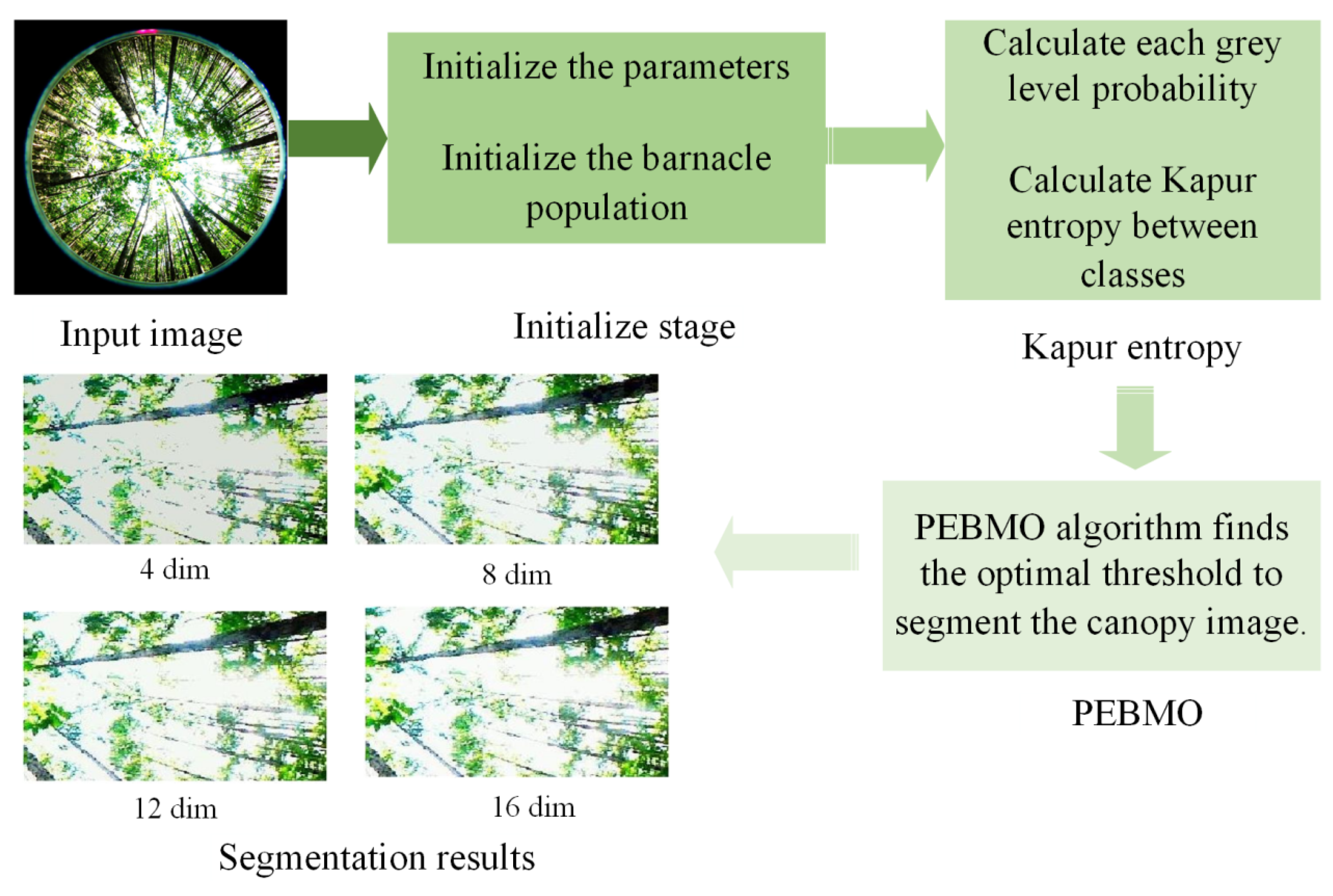
In order to improve the segmentation performance of the canopy image, Kapur entropy is the fitness function, and the PEBMO algorithm searches for the optimal threshold to segment the canopy image accurately. Figrue Figure 5 shows the flowchart of the proposed multi-threshold segmentation of the canopy image based on the PEBMO algorithm. The framework of the proposed algorithm is as follows:

1. Input the image to be segmented.

2. Generate the population and parameters of PEBMO.

3. Calculate each grey level’s probability (22).

4. Calculate the fitness value of each search agent by using (19) for Kapur entropy.

5. PEBMO algorithm finds the optimal threshold to segment the canopy image.

6. Output the segmentation result.

3. Results

This section consists of two parts: the testing and validation of the PEBMO algorithm’s performance and the testing and validation of the PEBMO-based segmentation algorithm.

3.1. Performance Testing and Analysis of the PEBMO Algorithm

3.1.1. CEC2017 Test Functions

CEC2017 is a collection of test functions used in the 2017 IEEE Congress on Evolutionary Computation (CEC) competition, and the essential information is shown in

Table 1. Basic information about CEC2017 test functions. * $F_2$ shows unstable behavior, especially for higher dimensions, and significant performance variations for the same algorithm implemented. For high-dimensional test functions, $F_2$ is usually excluded. Since this study is not a high-dimensional testing study, however, $F_2$ is also tested.

	No.	Functions	${\mathit{F}}_{\mathit{i}}^{*}={\mathit{F}}_{\mathit{i}}\left({\mathit{x}}^{*}\right)$
Unimodal Functions	$F_1$	Shifted and Rotated Bent Cigar Function	100
	$F_2$	Shifted and Rotated Sum of Different Power Function *	200
	$F_3$	Shifted and Rotated Zakharov Function	300
Simple Multimodal Functions	$F_4$	Shifted and Rotated Rosenbrock’s Function	400
	$F_5$	Shifted and Rotated Rastrigin’s Function	500
	$F_6$	Shifted and Rotated Expanded Scaffer’s Function	600
	$F_7$	Shifted and Rotated Lunacek Bi_Rastrigin Function	700
	$F_8$	Shifted and Rotated Non-Continuous Rastrigin’s Function	8000
	$F_9$	Shifted and Rotated Levy Function	900
	$F_{10}$	Shifted and Rotated Schwefel’s Function	1000
	$F_{11}$	Hybrid Function $1(\mathrm{N}=3)$	1100
	$F_{12}$	Hybrid Function $2(\mathrm{N}=3)$	1200
	$F_{13}$	Hybrid Function 3 ($\mathrm{N}=3$)	1300
Hybrid Functions	$F_{14}$	Hybrid Function 4 ($\mathrm{N}=4$)	1400
	$F_{15}$	Hybrid Function 5 ($\mathrm{N}=4$)	1500
	$F_{16}$	Hybrid Function 6 ($\mathrm{N}=4$)	1600
	$F_{17}$	Hybrid Function 6 ($\mathrm{N}=5$)	1700
	$F_{18}$	Hybrid Function 6 ($\mathrm{N}=5$)	1800
	$F_{19}$	Hybrid Function 6 ($\mathrm{N}=5$)	1900
	$F_{20}$	Hybrid Function 6 ($\mathrm{N}=6$)	2000
Composition Functions	$F_{21}$	Composition Function $1(\mathrm{N}=3)$	2100
	$F_{22}$	Composition Function 2 ($\mathrm{N}=3$)	2200
	$F_{23}$	Composition Function 3 ($\mathrm{N}=4$)	2300
	$F_{24}$	Composition Function 4 ($\mathrm{N}=4$)	2400
	$F_{25}$	Composition Function 5 ($\mathrm{N}=5$)	2500
	$F_{26}$	Composition Function 6 ($\mathrm{N}=5$)	2600
	$F_{27}$	Composition Function 7 ($\mathrm{N}=6$)	2700
	$F_{28}$	Composition Function $8(\mathrm{N}=6)$	2800
	$F_{29}$	Composition Function 9 ($\mathrm{N}=3$)	2900
	$F_{30}$	Composition Function 10	3000
Search Range: ${[-100,100]}^D$

. Among them, $F_1-F_3$ are single-peak functions containing only one global optimal solution, which are used to test the convergence speed and local search ability of the algorithm. $F_2$ shows unstable behavior, especially for higher dimensions, and significant performance variations for the same algorithm implemented. For high-dimensional test functions, $F_2$ is usually excluded. Since this study is not a high-dimensional testing study, however, $F_2$ is also tested. $F_4-F_{10}$ are multi-peak functions containing multiple local optimal solutions, which are used to test the exploration ability of the algorithms and the ability to jump out of the local optimal solutions. Such functions are adapted to test the performance of algorithms in solving complex multipeak optimization problems. $F_{11}-F_{20}$ are hybrid functions that contain multiple functions combined to create variety and complexity. $F_{21}-F_{30}$ are composite functions, which are combinations of various simple functions, each of which is univariate but combined to form a high-dimensional composite function. Hybrid and composite functions were used to solve large-scale optimization problems and test the potential of the algorithms to solve complex problems in the real world.

3.1.2. Experimental Setup

The experiment was conducted on a Dell Computer USA. The model number is the Alienware G15 5530 1526. It is configured for an Intel CPU @2.50 GHz, 16 GB of RAM, and a Windows 11 operating system. This equipment was purchased from Suihua, China. The PEBMO algorithm was compared with five BMO variants to verify its performance. The algorithm parameters are listed in

Table 2. Parameter setting for each algorithm.

Algorithm	Parameters Setting	Value
ABMO [32]	Penis length $pl$	7
IBMO [33]	Penis length $pl$	7
	LF index $\tau$	1.5
IBMO [34]	Maximother penis length $P_{\max }$	7
	Minimother penis length $P_{\min }$	1
	The initial decay rate $\lambda$	3
IBMO [35]	Penis length $pl$	7
	Gaussian distribution parameter $\lambda$	0.7
IBMO [36]	Penis length $pl$	7
	Parameters u	0.005
	Parameters v	0.5
	Parameters $\theta$	$[-2\pi ,2\pi ]$
	Linear decline factor $\delta$	[0, 1]
BMO	Penis length $pl$	7
PEBMO	Penis length $p{l}_1$	27

. The population size $\left(N\right)$ of the experiment was set to 30, and the maximum number of iterations $\left(T\right)$ was 500. Each benchmark function was independently run 30 times to avoid chance errors in the optimization search. The fitness value, standard deviation, and convergence curve were used as evaluation indexes. The best results are shown in bold font.

3.1.3. Sensitivity Analysis

In order to objectively analyze the influence of the changes of parameters N and T on the accuracy and stability of the PEBMO algorithm’s optimization search, a sensitivity analysis is carried out. Table 1 is used as the test function, and the average adaptability and standard deviation values are the evaluation indices. The average fitness values reflect the optimization accuracy of the algorithm. The standard deviation reflects the stability of an algorithm. The optimization accuracy and stability of the PEBMO algorithm are verified at different N and T values, respectively. Figure 6a shows the number of the optimal average fitness values and standard deviation values obtained by the PEBMO algorithm at different values of N. The figure shows that the PEBMO algorithm obtains 13, 10, 6, and 4 optimal average fitness values and 11, 10, 3, and 6 optimal standard deviation values when N is 30, 40, 50, and 60, respectively. No optimal fitness values and standard deviation values were obtained for N of 5, 10 and 20. This is due to the fact that the algorithm cannot fully explore the solution space when N is small, and the computational complexity increases when N is large. Therefore, neither too large nor too small N is conducive to the algorithm’s optimization search. It is worth noting that there are three sets of juxtaposed optimal values in obtaining the average fitness value, thus leading to more than 30 total optimal averages. Figure 6b shows the number of the optimal average fitness values and standard deviation values obtained by the PEBMO algorithm at different values of T. From the figure, it can be seen that the effect on the average fitness values is more significant at different T values compared to the standard deviation values. Thirteen optimal average fitness values and eight optimal standard deviation values were obtained at T = 500, which are better than the other T values.

To summarize, the parameters N and T affect the evaluation of the algorithm’s performance. Too large and too small N and T are not conducive to the algorithm performance test. The experimental results show that the PEBMO algorithm obtains the most optimal fitness values and standard deviation values when N = 30, which is 43.33% and 36.67% better than other particle numbers, respectively. As for the number of iterations, the PEBMO algorithm obtained 43.33% of the optimal average fitness value and 26.67% of the optimal standard deviation value when T = 500, which is better than other T values. Therefore, in the algorithm performance testing experiments, the number of population particles is N = 30, and the number of iterations is chosen as T = 500.

3.1.4. Analysis of Optimization Accuracy and Stability Score

Figure 7 and Figure 8 show the histograms of the distribution of the optimal mean fitness and number of standard deviation values for each BMO variant algorithm on the CEC2017 test function, respectively. The average fitness value reflects the optimization accuracy of the algorithm and the standard deviation value reflects its stability.

Figure 7 and Figure 8 show that, in comparison with the BMO variant algorithm, the PEBMO algorithm performs well in terms of seeking accuracy, $96.67\%$ better than the BMO variant algorithm, and $100\%$ better than the base BMO algorithm. This shows that the PEBMO algorithm has a high optimization accuracy and that the improvement of the PEBMO algorithm by each strategy is effective. PEBMO algorithm outperformed the comparison algorithm by $100\%$ in optimization accuracy on the single-peak function and $66.67\%$ stability. This is owing to the introduction of the dynamically decreasing reproduction coefficient p, which effectively improves the exploitation capability of the BMO algorithm. IBMO [33] and IBMO [35] also improved parameter p to improve its exploitation capability. As can be seen from the test results in

Table 3. Parameter setting for deep learning.

Parameter Name	Value
image size (img_size)	$256\times 256,264\times 264$
Patchsize (patch_size)	$4,8,12,16$
Embedding dimensions (embed_dim)	256,264
Transformer layer (num_layers)	4
Number of heads of the multiple self-attention
mechanism (num heads)	8
loss function	Cross - Entropy Loss
learning rate (learning_rate)	Adam
momentum parameter (betal and beta2)	Use default values
weight decay (weight_decay	1 × 10−4
Batch size (batch_size)	16
training wheels (epochs)	100

, the improvement effect is average and not as good as that of the other BMO variants of the algorithm.

The PEBMO algorithm has a more substantial optimization accuracy on the multipeak function, $85.7\%$ better than the comparison algorithm, indicating that the PEBMO algorithm has a strong global optimization ability and the ability to jump out of the local optimal solution. The BMO algorithm also performs well on the multipeak function, indicating that the BMO algorithm itself has good global optimization ability. To improve the global optimality-seeking ability of the BMO algorithm, IBMO [34] replaced $rand$ ( ) with the chaos vector obtained from the logistic chaos mapping, and IBMO [36] added coefficients to $rand$ ( ). The test results in Table 3 show that for the optimization of the multi-peak function, the optimization accuracy of IBMO [34] and IBMO [36] is not as good as that of the BMO algorithm, which is why this study does not improve the exploration phase of the BMO algorithm. The PEBMO algorithm outperforms the BMO algorithm because the extensive range of incremental penis coefficients, $pl$, provides a better balance between the exploration and exploitation of the BMO algorithm.

Chebyshev chaos perturbation at $pl=0.5$ allows the algorithm to jump out of the local optimal. Chebyshev chaotic perturbation, although it provides the PEBMO algorithm with a higher accuracy in finding the optimal on the multi-peak function, it also leads to less stability than IBMO [35]. IBMO [35] obtained optimal standard deviation values for $F_5,F_6$, and $F_7$, but their average fitness values were poor. This shows that the algorithm fails to effectively jump out of the local optimal solution for these three functions and falls into a precocious situation. In addition, IMBO [35] has a large stability gap for different functions and achieves optimal standard deviation values for $F_3,F_5,F_6,F_7,F_{20}$, and $F_{26}$. At the same time, it is almost the worst value for other functions, especially $F_2,F_{13},F_{15},F_{19}$, and $F_{30}$, which is inferior to other algorithms. This phenomenon also proves that the instability effect caused by the double disturbance was significant. However, whether the perturbation of IMBO [35] is strong or weak, its optimization search accuracy is not as good as that of the other algorithm variants.

The PEBMO algorithm has a significant advantage in hybrid and composite functions and is $100\%$ better than the comparison algorithms in terms of optimization accuracy. It is $60\%$ better than the comparison algorithm in terms of stability, and $75\%$ better than the BMO algorithm. This shows that the PEBMO algorithm is more comprehensive and has a high optimization accuracy and stability in optimizing large-scale and realistic problems, with obvious advantages.

3.1.5. Statistical Analysis

The Wilcoxon rank–sum test is a nonparametric statistical method for comparing differences between two independent groups of samples. Compared to the t-distribution test, Fisher’s exact test, and Kruskal–Wallis H test, it has the advantage of not requiring the assumption that the data obeys a specific probability distribution, is stable and unaffected by outliers, and is simple, convenient, intuitive, and easy to understand. Therefore, it is widely used to evaluate the differences between the performance of each algorithm. Where 0.05 is the significance level, a p-value greater than 0.05 indicates that the difference between the two groups is not significant, and a p-value less than 0.05 indicates that the difference between the two groups is significant. The Wilcoxon–rand rank sum test values for each algorithm are shown in Figure 9. Where the black horizontal line is the significance level value of 0.05, from the figure, it can be seen that the p-values obtained by the PEBMO algorithm in the determination of the differences with the other algorithms are less than 0.05, which indicates that the PEBMO algorithm has been significantly improved. In addition, there is no distribution of values on some functions (e.g., $F_1$–$F_4$), which is because the p-value obtained on this function is too small, much less than 0.05; therefore, it is not significantly represented in the graph.

3.1.6. Convergence Analysis

The convergence curve of the function can intuitively reflect the convergence speed, accuracy, and ability of each algorithm to jump out of the local optimal solution. Figure 10 shows the convergence curve of some functions, in which the horizontal axis indicates the number of iterations and the vertical axis indicates the value of the optimal fitness.

On the convergence curve of the single-peak function, it can be seen that the red PEBMO curve has apparent fluctuations in the middle and late iteration, indicating that even in the late iteration, the diversity of the population is not lost and still has a strong exploitation ability. On the convergence curve of the multi-peak function $F_6$, the fitness value of the PEBMO algorithm is not as good as that of IBMO [30], which is consistent with the data in Table 3. For $F_{10}$, the convergence curve of the PEBMO algorithm is at the bottom of all curves, indicating that its fitness value is better than that of the comparison algorithm. The PEBMO curve was located at the bottom of the hybrid and composite function convergence curves. It converges slowly in the late iteration, indicating that the PEBMO algorithm has high optimization accuracy and good stability.

3.2. Experimental Results and Analysis of Canopy Segmentation

3.2.1. Data Analyses

The forest canopy is intricate and complex, and the canopy images obtained by the fisheye lens often have quality problems, such as uneven illumination and loss of details. They also often have the limitation of low segmentation accuracy when segmenting the canopy images. Therefore, before segmenting the canopy image, this paper uses the literature [45] method to enhance different canopy images. The enhanced canopy images are shown in Figure 11, Figure 12, Figure 13 and Figure 14. Figure 11 shows two different types of nonuniform canopy images. Among them, the overall brightness of the LS1–LS3 images was low, and only a small part was in the exposure state. By contrast, the brightness of the LB1–LB3 images was not as high as that of LS1–LS3. However, the bright area is large; therefore, accurately segmenting the boundaries of the bright regions is an excellent test for the segmentation algorithm. Figure 12 shows the canopy images acquired under low-illumination conditions. The tone is dark, especially at low tree trunks, and it is easily misclassified as background. Figure 13 shows a canopy image acquired under strong sunlight, where intense sunlight blurs the treetops bordering the sky because of the sun’s reflection, and it is very easy to misclassify faint foliage as the sky. Figure 14 shows a canopy image acquired under normal lighting conditions. However, because of the acquisition method (elevation shot) and the forest gap, there was low brightness and unclear details at the low tree trunks, even under ideal lighting conditions.

3.2.2. Experimental Setup

In this section, segmentation experiments are conducted on Figure 11, Figure 12, Figure 13 and Figure 14 to evaluate the effectiveness of the proposed PEBMO algorithm on the multi-threshold segmentation of forest canopy images. The population size (N) was set to 30, maximum number of iterations $\left(T\right)$ was 500, and number of thresholds (dim) was set to $4,8,12$, and 16. To verify the effectiveness of PEBMO in the multithreshold segmentation of forest canopy images. The segmentation results of the PEBMO algorithm were compared with those of ABC, ChOA, CS, FPA, MA, IMA, and BMO. structural similarity index (SSIM), peak signal-to-noise ratio (PSNR), feature similarity index (FSIM), and subjective evaluation metrics were used to assess the quality of the segmentation results.

3.2.3. Image Evaluation Metrics

SSIM considers the characteristics of the human visual system by measuring the similarity between the original and segmented images in terms of brightness, contrast, and structural similarity [46]. The SSIM value is located in the interval [0, 1], and the larger its value, the more similar is the segmented image to the original image. The formula for calculating SSIM is as follows:

$$\mathrm{SSIM}(x,y)={\displaystyle \frac{\left(2{\mu }_x{\mu }_y+C_1\right)\left(2{\sigma }_{xy}+C_2\right)}{\left({\mu }_x^2+{\mu }_y^2+C_1\right)\left({\sigma }_x^2+{\sigma }_y^2+C_2\right)}}$$

(24)

$${\mu }_x={\displaystyle \frac{1}{RC}}\sum _{i=1}^R\sum _{j=1}^{C}X(i,j)$$

(25)

$${\sigma }_x^2={\displaystyle \frac{1}{RC-1}}\sum _{i=1}^R\sum _{j=1}^C{\left(X(i,j)-{\mu }_x\right)}^2$$

(26)

$${\sigma }_{xy}={\displaystyle \frac{1}{RC-1}}\sum _{i=1}^R\sum _{j=1}^C\left(X(i,j)-{\mu }_x\right)\left(Y(i,j)-{\mu }_y\right)$$

(27)

where ${\mu }_x$ and ${\sigma }_x$ denote the mean and variance of the original image, respectively; ${\mu }_y$ and ${\sigma }_y$ denote the mean and variance of the segmented image; and ${\sigma }_{xy}$ is the covariance between the original image and the segmented image; and $C_1,C_2$ and $C_3$ are constants. $C_1=(0.01\ast L)2$, $C_2=(0.03\ast L)2,C_3=C_2/2,l=255$.

PSNR is the ratio of an image’s maximum possible pixel value to the minimum pixel difference caused by noise in the image [47]. Its magnitude directly depends on the intensity of the image. The larger the PSNR value, the more significant the noise-removal effect and the lower the image distortion [48]. The PSNR value was calculated as follows:

$$\begin{array}{c}PSNR=20·\log \left({\displaystyle \frac{255}{RMSE}}\right)\end{array}$$

(28)

$$\begin{array}{c}RMSE=\sqrt{{\displaystyle \frac{{\sum }_{i=1}^H{\sum }_{j=1}^W\left(I(i,j)-I^{\prime }(i,j)\right)}{H\times W}}}\end{array}$$

(29)

$I(i,j)$ and $I^{\prime }(i,j)$ are the original and segmented images, respectively, and H and W are the image dimensions.

FSIM is another method for assessing the feature similarity after SSIM [49]. Unlike SSIM, it measures image quality by evaluating the feature similarity between the original and segmented images. The better the image quality, the closer the value is to 1. The formula for the FSIM is shown in Equation (30).

$$FSIM={\displaystyle \frac{{\sum }_{x\in \Omega }{S}_L\left(x\right)\times P{C}_m\left(x\right)}{P{C}_m\left(x\right)}}$$

(30)

where $\Omega$ is the pixel value of the entire image, $S_L\left(x\right)$ denotes the similarity value, and $P{C}_m\left(x\right)$ represents the phase consistency measure.

$$P{C}_m\left(x\right)=\max \left(P{C}_1\left(x\right),P{C}_2\left(x\right)\right)$$

(31)

$P{C}_1\left(x\right)$ and $P{C}_2\left(x\right)$ denote the phase coherence of the reference and segmented images, respectively.

$$S_L\left(x\right)={\left[S_{PC}\left(x\right)\right]}^{\alpha }·{\left[S_G\left(x\right)\right]}^{\beta }$$

(32)

$$S_{PC}\left(x\right)={\displaystyle \frac{2P{C}_1\left(x\right)\times P{C}_2\left(x\right)+T_1}{P{C}_1^2\left(x\right)\times P{C}_2^2\left(x\right)+T}}$$

(33)

$$S_G\left(x\right)={\displaystyle \frac{2G_1\left(x\right)\times G_2\left(x\right)+T_2}{G_1^2\left(x\right)\times G_2^2\left(x\right)+T_2}}$$

(34)

where $S_{PC}\left(x\right)$ denotes the feature similarity of the image; $S_G\left(x\right)$ denotes the gradient similarity of the image; $G_1\left(x\right)$ and $G_2\left(x\right)$ represent the gradient magnitude of the reference image and the segmented image, respectively; $\alpha ,\beta ,T_1$ and $T_2$ are constants.

3.2.4. Image Segmentation Accuracy Analysis

The line graph of the fitness value obtained by each algorithm is shown in Figure 15. The fitness value effectively reflects the segmentation accuracy of the image. The larger its value, the higher the segmentation accuracy. From the figure, it can be seen that the fitness value fold is approximated as a triangular wave, indicating that the segmentation accuracy of each algorithm increases with the increase in the number of thresholds. When the number of thresholds is 4, the adaptation value of each algorithm is low, and the difference is not significant, indicating that none of the algorithms can segment the image accurately. As the number of thresholds increases, the gap between the algorithms is gradually apparent. The PEBMO algorithm has a clear advantage and is located at the top, indicating that its segmentation accuracy is better than the comparison algorithms. As shown in

Table A8. Optimal fitness values obtained by each algorithm.

Image	Dim	ABC	ChOA	CS	FPA	MA	IMA	BMO	PEBMO
LS1	4	48.0086	47.9661	47.7049	47.5568	48.0145	48.0159	48.0159	48.0159
	8	79.2815	78.4253	77.2884	77.1758	79.8274	79.82757	79.8011	79.8336
	12	104.7496	102.9617	101.5882	102.2865	106.2248	106.2445	105.2567	106.2499
	16	126.2755	123.3417	120.5088	121.867	129.0688	129.1405	129.0721	129.3424
LS2	4	48.318	48.264	48.1137	47.7903	48.3211	48.3252	48.3204	48.3238
	8	79.8587	79.299	77.8174	76.8721	80.4522	80.4494	80.4415	80.4532
	12	104.5855	102.9147	100.4812	100.7449	106.867	107.0246	105.1117	107.0272
	16	125.9141	124.7758	121.9272	120.6541	129.3555	129.8391	129.5242	129.9012
LS3	4	47.089	47.0635	46.8658	46.7165	47.0974	47.0974	47.0143	47.0974
	8	77.7139	77.3476	75.947	74.7763	78.3275	78.2703	78.3124	78.339
	12	102.1062	100.8328	97.3349	98.2392	103.7293	103.72	103.4798	103.6359
	16	123.2746	122.903	120.0128	120.8741	128.0451	127.6188	125.9931	127.9746
LB1	4	46.2099	46.1422	45.9228	45.7896	46.2168	46.2172	46.2168	46.2172
	8	76.2824	75.6662	73.7629	74.2691	76.9955	77.0169	76.13	77.0028
	12	101.1045	99.5656	97.6718	98.2685	102.7173	102.9983	102.8093	103.0667
	16	122.0963	121.4659	120.6648	117.8679	127.4983	128.2044	126.5449	127.6949
LB2	4	46.0391	45.9648	45.6301	45.5101	46.0496	46.0496	46.0483	46.0496
	8	76.9162	76.2294	75.0841	74.6257	77.5274	77.5943	77.491	77.596
	12	101.6975	101.3461	97.4157	98.2788	103.5888	103.7153	103.006	103.9161
	16	123.1056	121.6342	119.1038	120.5048	127.4749	127.1375	127.182	127.2849
LB3	4	49.081	49.0397	48.9094	48.631	49.0918	49.0918	49.0915	49.0918
	8	80.4904	79.8217	79.0943	77.1859	81.0314	81.0337	81.016	81.047
	12	105.2572	104.1442	101.7131	100.3685	107.6818	107.5712	107.3766	107.7648
	16	125.4144	125.4449	121.534	122.3018	130.4694	130.7899	129.6344	130.7112
L1	4	48.5012	48.4373	48.3292	47.9622	48.51	48.51	48.51	48.51
	8	80.0675	79.7374	78.6066	77.4614	80.6704	80.6945	80.6597	80.6946
	12	105.7694	105.1358	102.1743	102.7151	108.0408	107.7356	107.7697	108.0403
	16	127.7735	125.6091	125.4105	126.1313	131.6222	131.5283	131.8409	132.1093
L2	4	48.4221	48.3408	47.9585	48.1355	48.4322	48.4322	48.4322	48.4322
	8	80.4402	79.6785	78.0003	78.6101	80.9598	80.9672	80.9255	80.9789
	12	105.8806	105.632	103.7626	103.8049	108.3114	108.3499	108.3412	108.5285
	16	127.7982	126.5144	124.2342	125.7799	132.4709	132.5962	131.1821	132.6609
L3	4	47.7785	47.7218	47.531	47.2409	47.7874	47.7874	47.7874	47.7874
	8	79.5244	79.1182	77.575	77.0088	79.9421	79.9612	79.9567	79.9768
	12	105.1771	103.9931	103.0118	103.7187	107.4628	107.4741	107.2843	107.4685
	16	126.706	126.0217	126.1506	124.2492	131.3893	131.5671	130.75	131.5785
L4	4	49.1875	49.1585	49.0315	48.6721	49.1927	49.1927	49.1927	49.1927
	8	81.4676	81.2848	79.8282	79.317	81.9774	81.979	81.9695	81.9818
	12	107.5178	107.0374	105.0405	105.057	109.6753	109.6923	109.3656	109.7259
	16	129.5379	127.1497	124.2868	123.9073	133.6504	133.6855	133.2264	133.6386
S1	4	49.338	49.3001	48.9188	49.0775	49.3421	49.3421	49.3421	49.3421
	8	81.4013	80.9903	79.8724	79.9943	81.8839	81.8842	81.8731	81.8842
	12	107.2292	105.4543	104.5251	102.8939	108.842	109.1382	108.8739	109.1467
	16	128.408	127.7292	125.9984	123.7531	132.8784	133	132.465	132.8416
S2	4	39.1209	38.9972	38.5964	38.3374	39.1818	39.1782	39.1488	38.9676
	8	62.0115	61.3552	59.5001	59.9369	62.9102	63.0693	62.5815	62.3881
	12	78.7681	76.7631	73.3395	73.244	81.3689	81.5577	80.2543	78.3173
	16	89.8799	86.9816	84.7803	82.0442	96.2297	96.2723	91.8726	91.7885
S3	4	49.468	49.4192	49.1355	49.2403	49.4779	49.4779	49.4763	49.4779
	8	81.5856	81.4717	80.2728	79.1026	82.3089	82.3113	82.2931	82.3125
	12	107.6504	106.7669	105.3293	103.3981	109.5594	109.8243	109.6236	109.7859
	16	129.7214	126.7394	127.524	125.7382	133.478	133.679	132.2654	133.3721
S4	4	47.7766	47.7406	47.5347	47.3725	47.7835	47.7836	47.7835	47.7836
	8	79.5835	79.4014	77.3646	78.057	80.0262	80.0219	80.0264	80.0651
	12	106.0834	105.1352	103.3057	103.4634	107.7611	107.8908	107.7554	107.8515
	16	127.2673	126.7021	124.6762	125.0253	131.3905	132.014	130.9904	132.0132
N1	4	47.8655	47.8356	47.6618	47.5819	47.8747	47.8747	47.8743	47.8747
	8	79.799	79.4778	77.5963	78.3729	80.2989	80.3078	80.287	80.2688
	12	105.7812	104.1394	101.5682	104.6089	107.8763	107.8225	107.8454	107.9298
	16	127.3402	126.3404	124.1978	124.4306	131.7924	132.0332	131.1746	131.8597
N2	4	47.8495	47.8201	47.526	47.4187	47.856	47.856	47.8529	47.856
	8	105.8145	104.6116	103.3116	102.5263	107.5417	107.5732	107.5117	107.5868
	12	104.872	105.0269	101.9968	103.167	106.9648	107.307	106.6086	107.301
	16	127.37	126.7299	123.601	124.8646	131.0551	131.3882	129.7893	131.2023
N3	4	47.8233	47.7513	47.5664	47.5903	47.8288	47.8288	47.8286	47.8288
	8	79.817	79.4437	78.367	78.437	80.2674	80.2788	80.2493	80.276
	12	105.8145	104.6116	103.3116	102.5263	107.5417	107.5732	107.5117	107.5868
	16	127.2122	125.8929	125.1016	123.9052	131.2522	131.4418	130.6177	131.3901
N4	4	47.7639	47.7441	47.6013	47.4509	47.7752	47.7752	47.775	47.774
	8	79.8112	79.2091	78.241	77.9421	80.2766	80.2818	80.2677	80.2831
	12	105.4597	104.7805	102.5258	103.3431	107.6039	107.622	107.2717	107.6099
	16	127.0776	125.3874	122.243	123.5945	131.158	131.3819	130.6546	131.1936

in Appendix A, the improved algorithms IMA and PEBMO obtain 22 and 29 optimal adaptation values, respectively, accounting for $92.73\%$, while MA obtains the other two optimal values. In addition, compared with the essential MA and BMO algorithms, IMA and PEBMO improved $81.36\%$ and $90.9\%$ in segmentation accuracy, respectively. It shows that the improvement of algorithm performance can effectively improve the segmentation accuracy of canopy images. In the comparison between IMA and PEBMO, the PEBMO algorithm is $56.36\%$ better than IMA, indicating that the segmentation accuracy of the PEBMO algorithm is better than the IMA algorithm.

3.2.5. Image Segmentation Stability Analysis

The line graph of the standard deviation values obtained by each algorithm is shown in Figure 16. The standard deviation values reflect the stability of the algorithms. The lower its value, the higher the stability. As can be seen from the graph, the PEBMO algorithm has apparent advantages, except for the noticeable fluctuation in the S4 image with eight thresholds. It is located at the lowest end on all other images, which indicates that it has strong stability in segmenting the canopy image. As can be seen from

Table A9. Standard deviation values obtained by each algorithm.

Image	Dim	ABC	ChOA	CS	FPA	MA	IMA	BMO	PEBMO
LS1	4	9.5913E-04	8.1216E-02	6.6639E-02	4.3741E-02	3.3326E-02	2.2291E-02	1.2497E-03	1.0414E-02
	8	6.0017E-02	2.0291E-02	6.2622E-02	3.6112E-02	5.8858E-02	4.3839E-02	3.1330E-02	2.5475E-02
	12	3.1345E-02	6.7002E-02	8.1548E-02	4.3356E-02	9.4256E-02	5.3314E-02	3.5781E-02	3.4839E-03
	16	2.1172E-01	4.3651E-02	7.8594E-02	8.5891E-02	6.5116E-02	6.0465E-02	5.5038E-02	4.6511E-03
LS2	4	9.9558E-02	4.1407E-03	4.0976E-02	5.6743E-03	6.6753E-03	2.0703E-03	2.9489E-03	1.0351E-03
	8	4.7812E-02	5.6159E-02	5.7359E-02	7.7959E-02	3.9974E-02	1.0355E-02	3.0926E-02	1.7269E-02
	12	4.0536E-02	5.7343E-02	5.6543E-02	7.7624E-02	8.8753E-02	5.5329E-02	5.0172E-02	2.7418E-02
	16	4.5392E-02	5.6343E-02	5.8725E-02	673624E-02	8.3723E-02	8.0915E-02	7.5231E-02	2.6332E-02
LS3	4	7.5542E-03	6.7764E-03	6.7653E-02	6.5531E-02	5.6642E-01	3.8864E-02	2.7784E-02	2.3354E-03
	8	4.7753E-02	7.6534E-02	8.8253E-02	6.8843E-02	6.8263E-02	3.8862E-04	2.0032E-02	1.6603E-02
	12	3.7735E-02	5.7363E-02	6.8826E-02	7.9272E-02	6.6253E-02	6.8262E-02	3.7724E-02	2.8028E-02
	16	4.7363E-01	6.9273E-02	6.5615E-02	7.8223E-02	8.6635E-02	4.7363E-02	5.3836E-02	3.9038E-02
LB1	4	1.2346E-02	6.0606E-02	5.8373E-01	4.7364E-03	4.8834E-03	6.7736E-04	6.6363E-03	6.4921E-03
	8	5.7754E-02	6.7734E-02	73635E-02	8.6637E-02	5.7733E-02	4.8836E-02	3.6625E-02	1.8181E-02
	12	2.9734E-02	4.8836E-02	1.0050E-02	5.8836E-02	7.8853E-02	5.7733E-02	4.9835E-02	1.7339E-02
	16	2.8875E-01	4.9986E-02	6.9958E-02	6.8874E-02	5.7765E-02	5.9987E-02	4.9973E-02	4.4096E-02
LB2	4	1.7464E-02	8.7464E-01	8.7363E-03	1.3032E-03	2.8836E-02	2.9983E-02	1.9383E-01	1.8336E-03
	8	5.7736E-02	4.7764E-02	5.9974E-02	7.9986E-02	5.9982E-02	3.6684E-02	3.8862E-02	1.6774E-02
	12	7.6648E-02	5.7753E-02	4.9972E-02	6.8874E-02	5.8845E-02	4.9935E-02	3.0093E-02	2.5025E-02
	16	1.9927E-01	5.9942E-02	6.8845E-02	7.9974E-02	4.0083E-02	5.9973E-02	4.9984E-02	3.9933E-02
LB3	4	1.1266E-02	5.0096E-01	4.8971E-03	3.8875E-02	3.9985E-02	4.0097E-02	5.8876E-02	1.2222E-02
	8	7.8874E-02	7.9945E-02	9.8875E-02	5.9984E-02	6.7789E-02	8.9975E-02	3.9984E-02	1.7262E-02
	12	6.9986E-02	6.9975E-02	9.9983E-02	5.9985E-02	6.0096E-02	2.8865E-02	4.0086E-02	3.3675E-02
	16	5.8875E-02	7.8874E-02	8.0096E-02	7.0065E-02	5.9985E-02	4.9975E-02	3.7008E-02	2.5764E-02
L1	4	1.0515E-02	8.6635E-02	7.8836E-03	5.8863E-03	4.8836E-03	3.8836E-02	2.0036E-01	1.0309E-03
	8	7.8837E-02	6.9973E-02	6.0083E-02	1.2394E-02	5.7639E-02	4.0082E-02	3.9927E-02	1.7553E-02
	12	4.8837E-02	5.8837E-02	8.0083E-02	4.9937E-02	5.9937E-02	1.9973E-02	3.6645E-02	2.3773E-02
	16	4.9947E-01	6.0937E-02	5.0093E-02	6.8836E-02	9.8736E-02	7.9937E-02	4.9937E-02	2.1343E-02
L2	4	1.2636E-02	1.0526E-02	8.8837E-01	6.8837E-01	5.9937E-01	6.0038E-01	8.9936E-01	2.8888E-03
	8	5.9954E-02	7.7732E-02	4.9974E-02	5.0085E-02	6.0085E-02	4.0999E-05	2.9776E-02	1.4833E-02
	12	4.0096E-02	6.9985E-02	6.9999E-02	5.7732E-02	2.5806E-02	3.9975E-02	3.1432E-02	2.9094E-02
	16	2.0997E-01	4.8875E-02	4.9874E-02	6.9958E-02	6.8864E-02	3.8874E-02	5.8874E-02	3.1204E-02
L3	4	1.5297E-02	8.9951E-02	7.8875E-02	4.9986E-01	4.8753E-01	2.2986E-01	2.0097E-01	1.8831E-03
	8	4.7764E-02	9.9975E-02	7.0085E-02	8.0084E-02	5.7753E-02	4.8853E-02	1.3764E-02	9.8874E-02
	12	3.8846E-02	5.8474E-02	6.8846E-02	5.8456E-02	8.0048E-02	6.0048E-02	4.0484E-02	2.3032E-02
	16	3.9634E-02	5.8846E-02	6.9937E-02	6.8836E-02	8.9937E-02	4.0938E-02	3.3037E-02	2.9874E-02
L4	4	9.5567E-03	6.8474E-02	7.9938E-02	5.0847E-02	4.9937E-01	3.9374E-01	2.4746E-01	1.0162E-03
	8	4.9975E-02	5.9974E-02	8.8874E-02	7.8863E-02	6.9975E-02	7.2312E-03	8.9984E-03	7.7937E-03
	12	4.9977E-02	6.9937E-02	8.9937E-02	6.0083E-02	4.0037E-02	8.0037E-02	4.9373E-02	2.2557E-02
	16	4.0085E-02	8.8852E-02	4.0964E-02	7.8853E-02	6.9964E-02	4.8863E-02	3.0874E-02	2.4199E-02
S1	4	9.3306E-03	8.8751E-03	6.0085E-02	5.9974E-01	4.9986E-02	2.9987E-01	3.0096E-02	1.0131E-03
	8	6.0096E-03	5.0086E-03	8.9985E-03	7.0096E-03	4.0096E-03	3.7799E-03	4.0986E-03	3.9973E-03
	12	5.8863E-02	9.8866E-02	7.8864E-02	4.9974E-02	6.9984E-02	7.0085E-02	3.0654E-02	2.4505E-02
	16	4.9975E-02	5.0974E-02	7.9974E-02	9.8864E-02	5.8874E-02	6.9985E-03	5.0094E-02	3.3372E-02
S2	4	6.9986E-02	7.9974E-02	5.8864E-02	6.9962E-02	1.2251E-02	8.9984E-02	7.6543E-02	5.3598E-02
	8	4.6547E-02	7.9734E-02	5.0936E-02	4.9464E-02	8.8464E-02	5.0494E-02	4.0383E-02	2.0789E-02
	12	4.0986E-02	5.0986E-02	6.8754E-02	5.3096E-02	6.0974E-02	5.0964E-03	4.2132E-02	3.0986E-02
	16	5.0843E-02	7.0886E-02	7.3124E-02	6.0864E-02	5.9753E-02	4.0986E-02	3.2643E-02	2.7643E-02
S3	4	8.6991E-03	7.7647E-03	7.0837E-03	4.7474E-03	2.9384E-01	2.9336E-02	2.2393E-02	1.6162E-03
	8	5.8764E-02	7.9642E-02	6.2345E-02	5.2364E-02	4.3425E-02	3.6742E-02	1.0974E-01	1.0935E-02
	12	4.0875E-02	5.9865E-02	4.8657E-02	6.8464E-02	6.0383E-02	4.0293E-02	2.7397E-02	3.0854E-02
	16	3.0384E-01	5.0484E-02	6.0383E-02	4.9373E-02	7.4041E-02	6.0827E-02	3.0283E-02	2.4372E-02
S4	4	9.2204E-03	8.3636E-03	6.2467E-03	6.3029E-02	3.2038E-01	2.4038E-01	1.4735E-01	1.4647E-03
	8	4.8753E-02	7.9764E-02	7.8975E-02	5.0975E-02	4.9543E-02	1.7478E-02	9.0985E-02	2.4906E-01
	12	7.6753E-02	6.9854E-02	8.5753E-02	9.6425E-02	6.9876E-02	5.0861E-03	4.6874E-02	2.8757E-02
	16	3.9865E-02	5.1352E-02	6.3548E-02	6.1253E-02	8.0913E-02	7.2414E-02	6.0164E-02	2.7668E-02
N1	4	8.1573E-03	7.2837E-03	7.3928E-03	3.2283E-01	3.0393E-02	2.9303E-02	2.5039E-02	1.6701E-03
	8	4.8765E-02	8.9753E-02	6.8754E-02	6.7542E-02	5.8654E-02	1.6864E-02	1.8444E-01	1.8973E-02
	12	5.0764E-02	7.8753E-02	8.9753E-02	7.0864E-02	5.1531E-02	5.3642E-02	4.2742E-02	2.9642E-02
	16	2.7839E-01	5.2093E-02	5.5837E-02	7.3836E-02	7.1037E-02	1.8363E-02	4.3974E-02	3.3247E-02
N2	4	1.3807E-02	1.0438E-02	7.8364E-03	5.2028E-02	4.9374E-02	2.0383E-01	2.5052E-03	2.4937E-02
	8	4.0384E-02	5.0384E-02	6.4863E-02	4.8645E-02	4.2018E-02	4.3927E-02	4.5937E-02	1.3767E-02
	12	4.2028E-02	7.0283E-02	7.3746E-02	8.8363E-02	7.5927E-02	5.8374E-02	3.2027E-02	1.9626E-02
	16	5.0373E-02	6.4303E-02	6.5927E-02	8.0274E-02	8.3484E-02	6.9273E-03	5.0273E-02	3.4351-02
N3	4	1.0879E-02	7.7373E-03	6.4746E-02	3.3648E-02	3.0393E-01	2.7393E-02	2.4938E-02	1.0453E-03
	8	5.3038E-02	7.3746E-02	8.2937E-02	6.0375E-02	4.6937E-02	5.9474E-02	3.8354E-02	1.2453E-02
	12	4.8645E-02	5.2937E-02	6.4373E-02	7.4528E-02	4.0384E-02	1.9745E-02	3.3046E-02	2.6977E-02
	16	4.0384E-02	5.8464E-02	5.2947E-02	6.0484E-02	8.3746E-02	4.0173E-02	3.6037E-02	2.6190E-02
N4	4	1.2159E-02	6.0682E-02	5.8262E-03	4.8373E-02	1.8832E-03	3.5838E-02	3.9453E-02	2.3846E-02
	8	6.9374E-02	7.1835E-02	7.7253E-02	6.9363E-02	5.6383E-02	4.9337E-02	3.6937E-02	1.2635E-02
	12	3.8363E-02	5.6383E-02	7.3725E-02	8.0373E-02	7.9373E-02	6.8332E-03	3.2984E-02	2.8832E-02
	16	4.7545E-02	5.9334E-02	6.3835E-02	7.3854E-02	4.7663E-02	4.0936E-02	3.6303E-02	2.3904E-02

, PEBMO obtains 55.56% of the optimal standard deviation value. This is due to the effective improvement in the performance of the PEBMO algorithm, which enables the PEBMO algorithm to segment all types of canopy images accurately. IMA, which is also an improved algorithm, however, only obtained 23.61% of the optimal values but outperformed MA by 79.17%, indicating the effectiveness of the improvement of the IMA algorithm as well. The ABC, ChOA, CS, FPA, MA and BMO algorithms, on the other hand, performed mediocrely, with optimal values of 1, 1, 2, 3, and 3, respectively.

3.2.6. Structural Similarity Analysis

The line graph of SSIM values obtained by each algorithm is shown in Figure 17. The SSIM value reflects the structural similarity between the segmented image and the original image. The larger its value, the better the quality of the segmented image. As the number of thresholds increases, the SSIM value increases, but the stability of the algorithms is poor on the N2 image. The FPA, MA, IMA, BMO and PEBMO algorithms all show higher SSIM values for low thresholds than for high thresholds, and this is due to the fact that the branches and leaves in the N2 image are intricate and more difficult to segment, which is more challenging for the algorithms. Therefore, an unstable fluctuation phenomenon occurs during segmentation. ABC, ChOA, and CS algorithms do not show any fluctuation. Still, their SSIM values are lower, which indicates that ABC, ChOA and CS fall into local optimal solutions in segmentation and fail to segment the image accurately. Overall, IMA and PEBMO algorithms have apparent advantages. As shown in

Table A10. SSIM values obtained by each algorithm.

LS1	4	0.7209	0.72041	0.70679	0.71316	0.7192	0.72365	0.72451	0.72366
	8	0.81394	0.81254	0.8159	0.8032	0.82009	0.82608	0.81812	0.82698
	12	0.86021	0.87064	0.89263	0.91309	0.89585	0.88353	0.90316	0.89082
	16	0.92534	0.93719	0.9052	0.94332	0.90512	0.92546	0.91668	0.95507
LS2	4	0.77999	0.77693	0.75927	0.78285	0.77617	0.77833	0.78099	0.7759
	8	0.85729	0.86113	0.86577	0.8381	0.85615	0.85905	0.85471	0.85818
	12	0.90617	0.87217	0.90774	0.91228	0.90354	0.89829	0.90026	0.93189
	16	0.92607	0.90026	0.92724	0.95448	0.93401	0.94814	0.94043	0.95487
LS3	4	0.70844	0.70338	0.68467	0.7068	0.70876	0.70875	0.70096	0.71061
	8	0.81385	0.81051	0.80819	0.80746	0.81686	0.8272	0.81795	0.84149
	12	0.90099	0.9152	0.91567	0.90829	0.91489	0.92039	0.92065	0.93225
	16	0.90983	0.89826	0.92373	0.9445	0.92906	0.94626	0.94148	0.94616
LB1	4	0.67413	0.67647	0.63471	0.66604	0.6755	0.67636	0.67655	0.67646
	8	0.80718	0.78172	0.81787	0.78877	0.80161	0.80412	0.82123	0.81574
	12	0.90259	0.89423	0.87223	0.91554	0.92326	0.91254	0.90375	0.92138
	16	0.93583	0.91194	0.92891	0.93286	0.94553	0.94941	0.94295	0.9513
LB2	4	0.71374	0.72897	0.68797	0.69843	0.71162	0.71147	0.7125	0.71154
	8	0.86059	0.82713	0.85647	0.83107	0.84257	0.84424	0.84883	0.84406
	12	0.92004	0.9099	0.89476	0.89494	0.91749	0.92029	0.91291	0.92354
	16	0.94308	0.9498	0.9415	0.93511	0.95108	0.95476	0.94685	0.961
LB3	4	0.7237	0.71715	0.73343	0.72454	0.72074	0.72069	0.72131	0.72078
	8	0.81763	0.80184	0.81218	0.82187	0.82209	0.82212	0.82128	0.82868
	12	0.87506	0.816	0.86323	0.87579	0.86494	0.88007	0.88103	0.89334
	16	0.91178	0.90782	0.91396	0.90424	0.90056	0.90849	0.91602	0.92955
L1	4	0.79944	0.78747	0.79309	0.80102	0.79911	0.79916	0.79915	0.7993
	8	0.88484	0.87513	0.88975	0.8719	0.88712	0.89344	0.89539	0.88715
	12	0.93672	0.91776	0.91026	0.92789	0.94223	0.93488	0.94229	0.94893
	16	0.92965	0.93076	0.93272	0.94774	0.95019	0.96024	0.95576	0.96085
L2	4	0.78368	0.78069	0.76358	0.76148	0.78193	0.78171	0.78171	0.78185
	8	0.89037	0.87212	0.87899	0.87134	0.88128	0.883	0.88387	0.89283
	12	0.89247	0.90719	0.91242	0.91067	0.92242	0.9302	0.92607	0.93647
	16	0.94157	0.92202	0.92002	0.93117	0.94762	0.95013	0.941 79	0.94609
L3	4	0.77518	0.76438	0.78455	0.77297	0.77418	0.77412	0.7742	0.77438
	8	0.85874	0.84941	0.85805	0.86547	0.86907	0.87367	0.86328	0.89335
	12	0.91441	0.92022	0.92322	0.91332	0.91776	0.93102	0.91909	0.93653
	16	0.93372	0.91368	0.92028	0.94585	0.9562	0.9555	0.93065	0.95704
L4	4	0.82196	0.81989	0.80929	0.82211	0.82327	0.82307	0.82312	0.8233
	8	0.89617	0.8993	0.88036	0.88761	0.90449	0.9038	0.90383	0.90422
	12	0.92658	0.92037	0.91277	0.90874	0.92958	0.93158	0.92902	0.93037
	16	0.92118	0.92259	0.92976	0.93377	0.94642	0.94943	0.94629	0.94519
S1	4	0.79044	0.78916	0.78278	0.77501	0.79026	0.79007	0.79019	0.7902
	8	0.86464	0.86199	0.84322	0.86664	0.87537	0.87562	0.87544	0.87566
	12	0.90922	0.8849	0.91588	0.92138	0.92267	0.92023	0.92559	0.91965
	16	0.93986	0.94155	0.9165	0.94261	0.93625	0.94349	0.94236	0.94215
S2	4	0.74587	0.74563	0.76359	0.73645	0.7555	0.75683	0.75723	0.75167
	8	0.85443	0.82264	0.80746	0.84623	0.84835	0.86039	0.85681	0.85417
	12	0.9096	0.87075	0.88171	0.8445	0.91162	0.89509	0.9075	0.91285
	16	0.90528	0.88803	0.92328	0.91175	0.9302	0.93878	0.93332	0.93576
S3	4	0.83177	0.82701	0.81709	0.83111	0.83133	0.83119	0.83129	0.83128
	8	0.89552	0.89054	0.87439	0.90022	0.90632	0.90661	0.90491	0.90588
	12	0.91878	0.91021	0.90511	0.91017	0.93189	0.93398	0.93484	0.93149
	16	0.93203	0.92656	0.92255	0.93413	0.9432	0.94329	0.94434	0.94727
S4	4	0.8326	0.83271	0.81437	0.82581	0.83299	0.83305	0.83293	0.83328
	8	0.91445	0.91145	0.87831	0.90492	0.91652	0.91658	0.91428	0.91647
	12	0.93988	0.93424	0.92756	0.92549	0.94712	0.94898	0.94369	0.94795
	16	0.95606	0.94156	0.94257	0.94812	0.96009	0.95985	0.94511	0.94685
N1	4	0.82476	0.82638	0.82013	0.81048	0.82404	0.82372	0.82368	0.82384
	8	0.90785	0.90836	0.90864	0.90145	0.90909	0.90966	0.90221	0.90609
	12	0.93165	0.93162	0.94224	0.92944	0.94764	0.94846	0.94766	0.94679
	16	0.94201	0.9468	0.9411	0.93828	0.96164	0.96478	0.95875	0.96024
N2	4	0.84303	0.8388	0.84121	0.83065	0.84145	0.84262	0.84196	0.84162
	8	0.95053	0.93447	0.93441	0.95303	0.95881	0.95519	0.9574	0.95759
	12	0.93823	0.9443	0.93118	0.9382	0.95049	0.95317	0.95881	0.9509
	16	0.95628	0.94914	0.94013	0.9595	0.96596	0.97214	0.9584	0.96962
N3	4	0.85748	0.84639	0.8571	0.8506	0.8572	0.85702	0.85691	0.8598
	8	0.92271	0.91404	0.90503	0.92103	0.92691	0.92832	0.92819	0.92725
	12	0.95053	0.93447	0.93441	0.95303	0.95519	0.95881	0.9574	0.95759
	16	0.95666	0.94329	0.94722	0.96194	0.96935	0.96942	0.96693	0.96697
N4	4	0.84067	0.84131	0.82968	0.82762	0.8367	0.83668	0.83753	0.83606
	8	0.91293	0.90312	0.90426	0.91402	0.91399	0.91516	0.91106	0.9127
	12	0.93876	0.93478	0.93471	0.94267	0.94439	0.94629	0.94618	0.95286
	16	0.94471	0.93488	0.95145	0.95583	0.96163	0.97338	0.9565	0.96398

, the IMA and PEBMO algorithms obtain 63.89% of the optimal SSIM values. The advantages of IMA are concentrated on S1–S4 and N1–N4. The PEBMO algorithm outperforms the comparison algorithm on LS1–LS3, LB1–LB3, and L1–L4 images, whereas it is significantly inferior to IMA on S1–S4 and N1–N4 images. This indicates that the PEMBO algorithm is not as good as the IMA algorithm in segmenting strong and normal light canopy images.

3.2.7. Analysis of Image Distortion Level

The line graph of PSNR values obtained by each algorithm is shown in Figure 18. The PSNR values reflect the degree of distortion of the segmented image. From the graph, it can be seen that the IMA and PEBMO algorithms have a clear advantage and are located at the top of the image, indicating that their segmented canopy images are less distorted and of better quality. The excellent performance of the IMA and PEBMO algorithms is due to the effective improvement of the MA and BMO algorithms. On the L1–L4 images, the segmentation stability of the algorithms is high, and there is no apparent fluctuation. In addition, as shown in

Table A11. PSNR values obtained by each algorithm.

Image	Dim	ABC	ChOA	CS	FPA	MA	IMA	BMO	PEBMO
LS 1	4	17.6233	17.5314	16.7462	17.6533	17.6233	17.6546	17.6227	17.6314
	8	22.6606	22.2666	21.3939	20.7137	22.1226	22.3241	23.275	21.2806
	12	24.7934	25.3982	25.1572	24.721	24.8754	24.3582	25.4977	25.5312
	16	28.4347	27.2658	26.3327	28.0931	26.5375	27.1182	26.5893	28.9935
LS2	4	17.3107	17.5656	15.5857	17.6138	17.4985	17.1321	16.7503	17.138
	8	23.5077	23.4514	20.7865	21.328	21.5137	21.5287	21.5068	21.5758
	12	26.3244	23.2305	25.5912	24.9803	24.544	24.5541	26.4788	24.7528
	16	27.0119	26.2853	25.867	26.5227	26.0105	26.7947	26.3838	28.2071
LS3	4	16.899	16.5886	16.8356	16.9682	16.9008	16.9066	16.4037	16.936
	8	22.638	22.7319	21.7719	21.7665	23.1613	22.7127	23.2133	23.6906
	12	23.9628	26.7086	25.8549	24.0146	26.9739	25.3499	27.5647	27.1342
	16	27.8686	27.6627	27.0907	27.975	28.6953	30.9185	30.0886	28.9575
LB1	4	16.347	16.3106	14.5494	15.8343	16.338	16.3679	16.3628	16.3735
	8	22.3389	20.7777	23.0246	20.396	22.0868	22.2374	22.9416	22.8365
	12	27.0492	25.7607	24.4119	25.4867	28.7167	27.8912	28.058	27.5096
	16	27.961	27.6693	27.2149	28.3347	30.3771	30.7835	30.373	30.7994
LB2	4	17.0365	17.646	16.0829	16.3367	17.0308	17.0229	17.0404	17.0288
	8	24.3443	22.2848	23.4562	21.9288	22.8195	22.8411	22.9015	22.8438
	12	27.1613	26.1043	24.029	25.6698	26.2325	26.2385	26.7604	27.1785
	16	27.8746	28.593	27.2179	26.7854	28.1259	28.3738	29.3956	29.9283
LB3	4	16.521	17.0229	16.3612	16.5709	16.5641	17.1904	16.5184	16.5772
	8	22.7803	22.5045	21.5908	21.4871	23.5517	22.5135	23.53	22.5442
	12	24.3849	23.2298	22.2403	22.7708	24.0018	24.2922	25.9828	26.7508
	16	26.97	27.5437	26.7835	26.2494	26.5026	26.6673	25.9095	27.9759
L1	4	19.0818	18.8724	16.6503	19.2056	19.0971	19.1177	19.1174	19.1248
	8	23.9845	23.7547	20.7953	22.7214	25.1535	24.9971	25.1872	24.934
	12	26.7557	26.8244	24.0943	26.3993	28.474	28.7492	27.897	28.4827
	16	29.344	27.8012	26.5161	29.6275	30.2466	30.6045	30.2709	30.9262
L2	4	19.214	18.934	18.4822	18.2934	19.28	19.2661	19.2314	19.2611
	8	24.6821	23.9745	24.3752	23.2947	25.1417	25.1001	25.1898	25.2418
	12	26.9997	26.8935	25.6933	26.6686	28.648	28.6753	28.3863	28.7201
	16	28.4252	29.0059	26.8518	28.3103	30.9197	31.2622	29.8385	31.3071
L3	4	19.0855	18.6216	19.863	18.5664	19.1691	19.1448	19.1571	19.1681
	8	24.4603	24.3383	22.1891	22.079	24.6038	24.894	24.7713	24.9318
	12	27.6851	25.8301	26.9509	27.8983	28.4691	28.6442	28.4195	28.4659
	16	29.1044	28.6716	26.3205	28.7242	30.5994	30.9194	30.052	31.1223
L4	4	18.8011	18.8275	19.1015	18.4389	18.8672	18.84	18.8983	18.8256
	8	24.4402	24.5406	21.7447	23.6505	25.047	25.0946	24.9973	25.1384
	12	24.8287	26.9375	25.683	27.1285	28.5027	28.5998	27.7892	28.6067
	16	27.3812	28.5217	25.7337	26.4747	30.7057	30.8145	29.6389	30.9529
S1	4	18.8215	18.8977	18.7729	18.7698	18.9078	18.8915	18.8955	18.9285
	8	24.9591	24.6393	23.2686	23.8365	25.1517	25.1536	25.1225	25.0951
	12	27.0805	26.9384	23.8944	26.6772	28.2633	28.5538	28.2944	28.7182
	16	28.2425	28.255	28.0888	29.7205	30.9566	31.1797	30.5167	31.1172
S2	4	20.5159	20.2824	20.4582	20.2603	20.7525	20.8226	20.6059	20.5969
	8	24.9453	24.3096	23.6766	25.3071	25.4971	25.9313	26.019	26.2151
	12	28.0797	26.4541	26.1149	25.1395	29.0762	28.6297	29.1504	28.7945
	16	29.1548	28.1465	28.3377	29.8636	30.6961	31.3226	29.9611	31.1449
S3	4	18.5082	17.8457	17.403	18.3808	18.2577	18.1328	18.1228	18.241
	8	23.0315	21.7351	21.3589	23.4432	23.2565	23.5103	22.9768	23.7055
	12	24.8746	27.2904	23.8472	24.57	27.146	28.2448	27.3182	27.9499
	16	26.7708	28.3615	27.2307	29.5579	29.7832	30.4554	27.6182	29.7469
S4	4	18.2151	19.0337	17.7096	18.0413	18.3834	18.4671	18.3932	18.4992
	8	23.9811	24.4487	23.28	22.4472	25.036	25.0792	24.2885	24.8859
	12	27.1415	26.9	24.3046	27.6016	28.466	28.3352	28.135	28.5991
	16	28.1777	29.4093	26.5124	29.4189	31.0545	31.1967	30.5662	31.1365
N1	4	19.5422	19.2234	18.9259	18.8318	19.4357	19.3821	19.3507	19.3989
	8	24.4604	23.6524	24.4041	24.8512	25.3394	25.3609	25.2308	25.5503
	12	26.8013	27.3504	26.4697	25.9722	28.4772	28.0926	28.3457	28.4018
	16	28.5226	28.4434	27.7891	28.9198	30.3835	30.6952	30.4121	30.9756
N2	4	18.6177	18.4094	18.453	17.8951	18.6733	18.6819	18.5012	18.7055
	8	27.3798	27.0411	25.7212	26.9315	28.5073	28.6977	28.6039	28.6595
	12	26.5124	26.3507	24.4956	26.6851	28.6239	28.0661	27.7979	28.3443
	16	28.8253	27.9491	25.2474	27.5651	30.6305	30.8572	29.4339	30.6594
N3	4	19.4139	19.3445	19.6787	18.7282	19.4707	19.4034	19.4296	19.4436
	8	24.7077	24.4412	24.6671	24.5945	25.1031	25.3984	25.2439	25.139
	12	27.3798	27.0411	25.7212	26.9315	28.5073	28.6977	28.6039	28.6595
	16	29.555	27.8668	26.1534	29.2765	30.6679	31.2805	29.7968	31.2565
N4	4	19.1838	19.5107	19.4319	19.2365	19.3237	19.293	19.3566	19.4714
	8	24.197	24.9887	23.0143	23.1427	25.4654	25.4856	25.2843	25.503
	12	28.145	27.7777	27.1333	27.4841	28.7963	28.8931	28.418	28.7206
	16	27.6399	28.2612	27.0658	29.3758	30.5235	31.0846	30.5232	31.3229

, the IMA and PEBMO algorithms improved 72.22% and 76.39% in segmentation quality relative to the original algorithms, respectively. IMA only obtained three optimal values, although 75% better than the MA algorithm, which indicates that IMA is not good at segmenting non-uniform canopy images.

3.2.8. Feature Similarity Analysis

The line graph of FSIM values obtained by each algorithm is shown in Figure 19. From the figure, it is clear that the algorithms have obtained high FSIM values on all the images. Among them, it is higher than 0.83 on LS1–LB3 images, 0.94 on L1–L4 images, 0.93 on S1–S4 images, and 0.95 on L1–L4 images. This stems from the fact that the original image prior to segmentation has a better quality, and hence, enhancement before segmentation is necessary. As the number of thresholds increases, the FSIM value also increases. The advantage of the PEBMO algorithm is obvious: almost all of them are located in the topmost part of the image, which indicates that its segmented image is more similar to the original image in terms of structure and better quality. In addition, as shown in

Table A12. FSIM values obtained by each algorithm.

Image	Dim	ABC	ChOA	CS	FPA	MA	IMA	BMO	PEBMO
LS1	4	0.90224	0.90174	0.89546	0.89926	0.90196	0.90405	0.90409	0.9041
	8	0.93672	0.9336	0.93502	0.93176	0.93954	0.94219	0.94172	0.93919
	12	0.95426	0.95414	0.96394	0.97328	0.96679	0.96167	0.96977	0.96414
	16	0.97532	0.9796	0.9674	0.97651	0.96604	0.96866	0.97276	0.98245
LS2	4	0.90112	0.8985	0.88896	0.9012	0.89962	0.90013	0.90121	0.89825
	8	0.93886	0.9412	0.94092	0.92924	0.94088	0.94245	0.94006	0.94209
	12	0.96072	0.94495	0.95862	0.96385	0.96412	0.96055	0.96592	0.97683
	16	0.97139	0.95764	0.96885	0.98238	0.98078	0.98455	0.9844	0.98856
LS3	4	0.89401	0.88967	0.884	0.89446	0.89387	0.89408	0.88661	0.89708
	8	0.92676	0.92637	0.91353	0.93126	0.92803	0.93321	0.92822	0.9248
	12	0.95919	0.96649	0.98563	0.96223	0.96669	0.96924	0.96665	0.97563
	16	0.96898	0.96459	0.97436	0.98505	0.9761	0.98591	0.98052	0.98892
LB1	4	0.86394	0.86353	0.8401	0.85688	0.8643	0.86482	0.86473	0.86883
	8	0.91275	0.90385	0.92181	0.90043	0.90985	0.91104	0.92472	0.92137
	12	0.96626	0.96792	0.95296	0.97334	0.97212	0.97117	0.97108	0.96716
	16	0.98503	0.96931	0.97839	0.98462	0.98055	0.98858	0.9854	0.98844
LB2	4	0.8642	0.87295	0.84787	0.85671	0.8638	0.8638	0.8644	0.86379
	8	0.93962	0.92145	0.9361	0.92563	0.92847	0.93176	0.93309	0.93379
	12	0.97083	0.96287	0.95803	0.9588	0.96813	0.9695	0.96312	0.9669
	16	0.97817	0.9854	0.981	0.975	0.98444	0.98895	0.96975	0.98943
LB3	4	0.90716	0.90697	0.90315	0.90858	0.90619	0.90624	0.90647	0.90634
	8	0.94051	0.93447	0.93027	0.9423	0.94244	0.94231	0.94219	0.94239
	12	0.9583	0.9375	0.94954	0.95793	0.96112	0.95537	0.96346	0.96355
	16	0.9724	0.97079	0.97489	0.96988	0.96931	0.97198	0.97328	0.98367
L1	4	0.9627	0.95719	0.94878	0.96288	0.9628	0.96279	0.96282	0.96282
	8	0.98594	0.98302	0.97351	0.97948	0.96836	0.98678	0.98681	0.98875
	12	0.99431	0.99101	0.98694	0.99151	0.99621	0.99494	0.99569	0.99622
	16	0.99306	0.99256	0.99076	0.99536	0.99681	0.99751	0.9972	0.99871
L2	4	0.95749	0.95596	0.94837	0.94385	0.95669	0.95659	0.95664	0.95664
	8	0.98584	0.98281	0.98433	0.98187	0.98604	0.98648	0.98545	0.98578
	12	0.98725	0.98802	0.98849	0.98972	0.99287	0.99396	0.99472	0.99477
	16	0.99215	0.99198	0.98992	0.99345	0.99655	0.99667	0.99523	0.99819
L3	4	0.95823	0.95237	0.96312	0.95604	0.95826	0.9582	0.95823	0.95832
	8	0.98185	0.98015	0.98377	0.97917	0.98741	0.98643	0.98329	0.98641
	12	0.99142	0.99283	0.99303	0.99212	0.99404	0.99599	0.99634	0.9942
	16	0.99484	0.99129	0.99137	0.99547	0.99776	0.99874	0.99494	0.99897
L4	4	0.96317	0.96246	0.95986	0.96272	0.95402	0.96394	0.96407	0.96389
	8	0.98556	0.987	0.97843	0.98189	0.98929	0.98907	0.98917	0.98941
	12	0.98861	0.99026	0.98734	0.98688	0.99391	0.99454	0.99326	0.99366
	16	0.98787	0.99131	0.98513	0.98974	0.99599	0.99656	0.99554	0.99879
S1	4	0.95115	0.95088	0.94589	0.94119	0.95111	0.95212	0.95115	0.95106
	8	0.97816	0.97731	0.96718	0.97904	0.98265	0.98268	0.98257	0.98274
	12	0.98858	0.98262	0.98526	0.99114	0.993	0.99472	0.99341	0.99458
	16	0.99409	0.99314	0.98936	0.99481	0.99494	0.99884	0.99581	0.9978
S2	4	0.9395	0.9385	0.94141	0.93436	0.94467	0.94555	0.94427	0.94312
	8	0.98067	0.97174	0.96468	0.97705	0.97842	0.98027	0.98199	0.98426
	12	0.98958	0.98034	0.98161	0.96961	0.99083	0.98919	0.99022	0.9914
	16	0.98941	0.98725	0.98577	0.99098	0.994	0.9946	0.99215	0.99348
S3	4	0.94515	0.94072	0.93178	0.94404	0.94491	0.94493	0.94587	0.945
	8	0.97519	0.96943	0.95708	0.97672	0.98296	0.98332	0.98193	0.98288
	12	0.98426	0.98324	0.97335	0.98033	0.99152	0.99032	0.99177	0.98958
	16	0.98759	0.98746	0.98205	0.98842	0.99229	0.99237	0.99212	0.99383
S4	4	0.96278	0.96639	0.94911	0.95928	0.96379	0.96408	0.96373	0.96412
	8	0.98909	0.98857	0.97722	0.98396	0.99094	0.99596	0.99053	0.99111
	12	0.99429	0.99289	0.98742	0.98954	0.99549	0.99581	0.9952	0.99578
	16	0.99454	0.9934	0.99244	0.9944	0.99689	0.99819	0.99623	0.9974
N1	4	0.96412	0.9646	0.96037	0.95501	0.96372	0.96366	0.96345	0.96371
	8	0.98929	0.98811	0.98797	0.98782	0.98994	0.99015	0.98797	0.98866
	12	0.99294	0.99282	0.99327	0.99005	0.99607	0.99615	0.99614	0.99579
	16	0.99236	0.99338	0.99436	0.9923	0.99708	0.99736	0.99658	0.99707
N2	4	0.96161	0.95999	0.961	0.95489	0.96125	0.96113	0.96052	0.96124
	8	0.9936	0.9914	0.9897	0.99418	0.99605	0.99547	0.99584	0.99589
	12	0.99091	0.99216	0.98544	0.98951	0.99393	0.99488	0.99447	0.99547
	16	0.99468	0.9916	0.98601	0.99395	0.99647	0.99755	0.99477	0.99723
N3	4	0.97152	0.96657	0.97137	0.96818	0.97144	0.9713	0.97126	0.97139
	8	0.98881	0.98612	0.98494	0.98813	0.9907	0.99122	0.99046	0.99037
	12	0.9936	0.9914	0.9897	0.99418	0.99605	0.99547	0.99584	0.99589
	16	0.99528	0.99081	0.99105	0.99501	0.99725	0.99829	0.99678	0.99691
N4	4	0.97145	0.97279	0.96758	0.96568	0.97026	0.97031	0.97068	0.98052
	8	0.99051	0.98764	0.98609	0.9901	0.99042	0.99115	0.99069	0.99311
	12	0.99486	0.99302	0.99323	0.99418	0.99602	0.99624	0.98681	0.98617
	16	0.99316	0.99321	0.99496	0.99602	0.99766	0.998	0.97816	0.99788

, the optimal FSIM values are mainly distributed in MA, BMO, IMA and PEBMO algorithms, accounting for 81.94%. Among them, MA, BMO, IMA and PEBMO obtained 9.72%, 15.28%, 30.56% and 33.33% of the optimal values, while ABC, ChOA, CS and FPA obtained 6.94%, 2.78%, 2.78% and 5.56% of the optimal values, respectively.

3.2.9. Segmentation Efficiency Analysis

The computation time for each algorithm for various types of canopy images is shown in Figure 20, Figure 21, Figure 22 and Figure 23. Computation time reflects the segmentation efficiency of each algorithm. Overall, the magnitude of the computation time for each algorithm is $\mathrm{FPA}<\mathrm{CS}<\mathrm{CHOA}<\mathrm{BMO}<\mathrm{PEBMO}<\mathrm{ABC}<\mathrm{MA}<\mathrm{IMA}$. The computation time of the PEBMO algorithm is located at a medium level and inferior to that of BMO, which stems from the fact that to increase the probability of the BMO algorithm jumping out of the locally optimal solution, the parent generation of barnacle particles of $pl$ = 0.5 is subjected to the Chaos Perturbation of Chebyshev. The introduction of this link undoubtedly increased the running time of the PEBMO algorithm. However, the difference between the computational method times of the PEBMO and BMO algorithms was not significant. In addition, the time required by all the algorithms to increase from four dimensions to 16 dimensions is not more than 5 s, which also proves that the introduction of intelligent algorithms can effectively improve the limitations of the inefficiency of the multithreshold segmentation method.

3.3. Comparison of PEBMO and Deep Learning

3.3.1. Hyperparametric Analysis

In order to evaluate the PEBMO algorithm objectively and comprehensively, the segmentation results of the PEBMO algorithm are comprehensively compared with the deep learning segmentation method in terms of fitness values, standard deviation values, SSIM, PSNR, FSIM, and computation time. A Transformer segmentation module was used for deep learning. To analyze the effect of different hyperparameters (num_layers and $lr$) on the model performance. Hyperparameter analysis experiments were designed. Figure 24 shows the distribution of adaptation values, PSNR, SSIM, FSIM, computation time and standard deviation values for different $lr$ and num_layers conditions. The analysis and summary of Figure 24 is shown below:

(1) Effect of num_layers and learning rate ($lr$) on the Loss function

With the increase of num_layers, the Loss value shows an overall increasing trend. When num_layers = 2, the Loss is lower; while num_layers = 8, the Loss is higher. Increasing the number of layers may lead to overfitting of the model, especially when the amount of data is limited. A smaller learning rate ($lr$ = 0.0001) usually leads to lower Loss values.

(2) Effect of num_layers and $lr$ on PSNR

The value of PSNR is higher when num_layers = 2; it decreases as the number of layers increases. When num_layers = 2, the average PSNR value is greater than 62 for $lr$ = 0.0001; it decreases for num_layers = 8. Smaller learning rates ($lr$ = 0.0001) usually result in higher PSNR values. It is clearly seen that the FSNR values for $lr$ = 0.0001 are generally higher than the FSNR values for $lr$ = 0.01 and 0.001.

(3) Effect of num_layers and $lr$ on SSIM

Similar to PSNR, SSIM is higher for num_layers = 2; it gradually decreases as the number of layers increases, and the value of SSIM is generally higher when the learning rate $lr$ = 0.0001.

(4) Effect of num_layers and $lr$ on FSIM

In contrast to PSNR and SSIM, FSIM is lower for num_layers = 2; it gradually increases as the number of layers increases, and the value of SSIM is generally higher when the learning rate $lr$ = 0.01.

(5) Effect of num_layers and lr on computation time

The learning rate has a negligible impact on the computation time, and the average computation time is mainly affected by num_layers; the more num_layer layers there are, the longer the computation time will be.

(6) Standard deviation analysis

The standard deviation of Loss: A smaller $lr$ (e.g., $lr$ = 0.0001) usually results in a lower standard deviation, indicating more stable model training.

When num_layers is increased, the model may be overfitted, leading to an increase in Loss and a decrease in PSNR and SSIM. A smaller learning rate (e.g., $lr$ = 0.0001) usually leads to better performance and more stable training. Therefore, to ensure better time and model performance, this study uses the parameter combination num_layers = 4, $lr$ = 0.0001.

3.3.2. Analysis of Comparative Results

The relevant settings are listed in Table 3. The obtained segmentation results are shown in Figure 25, Figure 26, Figure 27, Figure 28 and Figure 29, respectively. It is worth noting that the gap between the deep learning method and the PEBMO algorithm is large in all the evaluation metrics; therefore, Figure 25, Figure 26, Figure 27, Figure 28 and Figure 29 are all double vertical axis bar charts. The left side is the vertical axis of the PEBMO algorithm and the right side is the vertical axis of deep learning.

As can be seen from the data in the table, there are significant differences between the deep learning segmentation algorithm and the PEBMO segmentation algorithm in several performance metrics. The advantages and disadvantages of deep learning and PEBMO algorithms are as follows:

1. Advantages of Deep Learning

(a) Deep learning segmentation methods generally have higher SSIM and PSNR values than the PEBMO algorithm at all thresholds. This indicates that deep learning algorithms are better able to capture the structural and feature information of an image, thereby providing higher-quality segmentation results.

(b) Deep learning is highly adaptable, can handle complex scene data, and has strong generalization ability. This makes it more advantageous for complex image segmentation tasks.

2. The shortcomings of Deep learning:

(a) It is less stable and susceptible to parameters that prevent it from maintaining consistent performance with different inputs.

(b) Although it outperforms the PEBMO algorithm in terms of computation time for individual images, it takes longer to compute at high thresholds and requires high-performance hardware support. This may limit their use in real-time applications.

(c) The data dependency is strong and requires a large amount of labelled data for training, which requires high data quality. If the data is insufficient or inaccurately labelled, the segmentation accuracy may be affected.

3. Advantages of the PEBMO algorithm:

(a) High segmentation accuracy: the optimal fitness value and FSIM value of the PEBMO algorithm under all thresholds are higher than that of the deep learning method, indicating that its segmented image has high segmentation accuracy and is more similar to the original image in terms of characterization.

(b) High stability: the PEMBO algorithm outperforms deep learning in terms of standard deviation values for all numbers of thresholds, indicating strong segmentation stability.

(c) Computationally efficient: shorter computation time, suitable for real-time applications.

(d) Simple and easy to implement: It does not require a large amount of training data suitable for simple scenarios.

4. Shortcomings of the PEBMO algorithm:

(a) Poor adaptability: significant performance degradation in low-dimensional or complex scenarios.

(b) The high degree of distortion: under all dimensions, the SSIM and PSNR values are generally lower than those of the deep learning algorithms, indicating that their segmentation results are not as good as those of the deep learning methods in terms of the degree of distortion.

3.3.3. Subjective Evaluation Analysis

Subjective evaluation can provide value that cannot be replaced by machines and can fully reflect how people feel about pictures in the real world. The segmentation results of each algorithm at threshold numbers 4, 8, 12 and 16 are shown in Figure 30, Figure 31, Figure 32 and Figure 33, respectively. The canopy image is intricate and complex, and it is inconvenient to observe how good or bad the segmentation is in the details. Therefore, the regions where the segmentation difficulties and error-prone points are located are intercepted on the segmentation result graphs for detailed analysis. In addition, due to the limitation of space, typical images from four different types of canopy images are selected for presentation.

From Figure 30, it can be seen that the segmentation quality of each algorithm is poor when the number of thresholds is 4. For the non-uniform canopy images LS1 and LB3, the difficulty of segmentation is in the light and dark junction; how to make the junction area accurately segmented is an excellent test for the algorithms. All the algorithms showed mis-segmentation, and some tiny branches and leaves were wrongly divided into the sky. The same is-segmentation also occurs in the N4 image; even though N4 is a normal illumination canopy image but limited by the shooting method (elevation), there are some uneven illumination phenomena in the ideal sample with uniform illumination, to a greater or lesser extent. On the low illumination canopy image L2, the algorithms misclassify the trees and branches at low places into the background. The strong illumination image S3 has the worst segmentation quality, which appears clear and blurred with low contrast. The FPA algorithm has the worst segmentation quality and shows severe colour distortion on both LB3 and S3.

The segmentation quality in Figure 31 is visually significantly better than in Figure 30. Some minute details have not yet been successfully segmented. The FPA algorithm shows a significant improvement in segmentation quality on LB3. While colour distortion still occurs on S3. The strong light image S3 is challenging for the segmentation algorithms. The ChOA, CS and FPA algorithms show colour distortion at a threshold number of 8. The segmentation results for threshold 12 and threshold 16 have little difference in subjective visualization, and the difference is hardly noticeable, which is also consistent with the objective evaluation index. As the number of thresholds increases, the computational complexity increases exponentially. It is more challenging for intelligent algorithms. The less-performing CS and FPA algorithms still cannot segment LB3 and S3 images accurately at high thresholds. While the other algorithms improve the segmentation quality significantly, the details hidden in the glare and darkness are accurately segmented. For example, on the L2 image, the trees at the lowest brightness can be accurately segmented, and the details of tree trunks, leaves, and ground are clearly visible.

The PEMBO algorithm demonstrates better segmentation quality and stability when segmenting different types of canopy images. Especially at low thresholds, better segmentation results can be obtained even when the comparison algorithms all show more serious segmentation errors. The PEBMO algorithm shows good stability and no colour distortion at any threshold.

4. Discussion

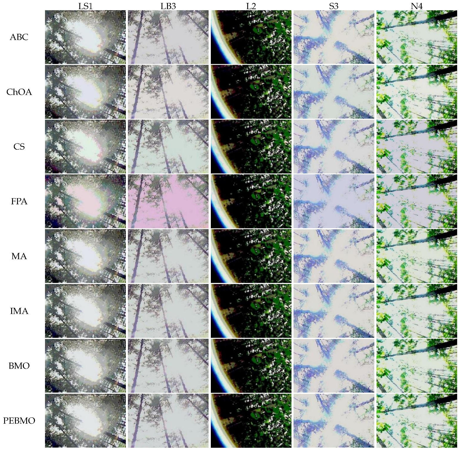
The results of the subjective and objective evaluations of each algorithm on the four types of forest canopy images show that the proposed PEBMO algorithm has obvious advantages over other intelligent algorithms and improved intelligent algorithms. The effectiveness of the improved PEBMO algorithm is demonstrated. However, there is no perfect algorithm to solve these problems. A canopy image has a significant gap in the complexity of the target, light intensity, and image clarity, which is a significant challenge to the accuracy and stability of image segmentation.

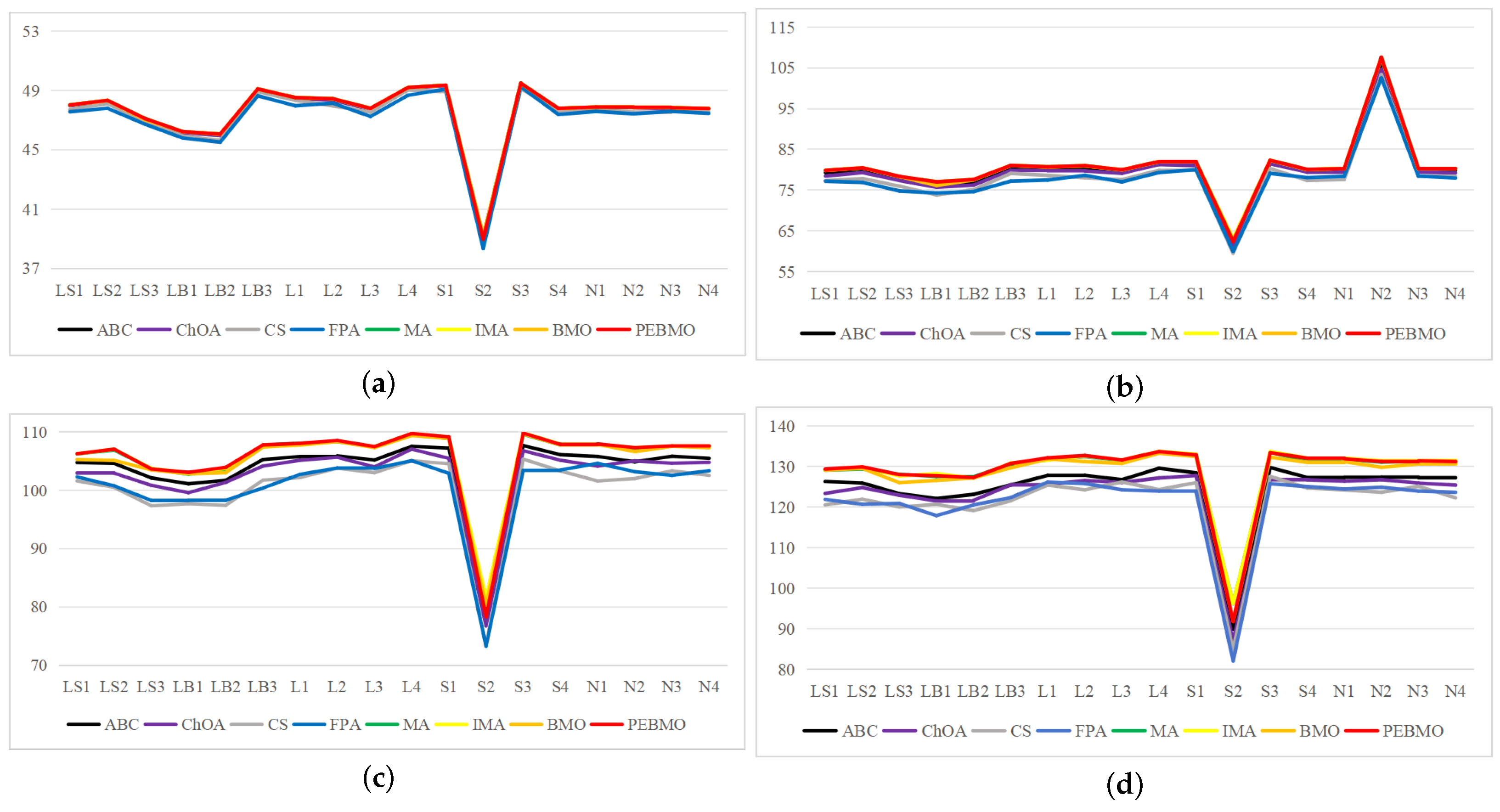
Image segmentation accuracy: 17 equal sets of optimal fitness values emerged in acquiring fitness values, of which 94.12% were distributed when the number of thresholds was 4. This stems from the fact that none of the algorithms can accurately segment the canopy image when the number of thresholds is not big enough, and the difference between the adaptative values obtained is insignificant. As the number of thresholds increases, the differences between the algorithms are gradually noticeable. The PEBMO and IMA algorithms have apparent advantages, 40.28% and 30.56% better than the other algorithms, respectively; 90.9% and 81.36% better than BMO and MA algorithms. It shows that it is necessary to improve the intelligent algorithms to improve the segmentation accuracy of canopy images. Although the PEBMO algorithm 56.36% outperforms IMA. However, the IMA algorithm outperforms PEBMO by 69.23% and 66.67% in segmenting strong and normal light canopy images. This indicates that the PEBMO algorithm has higher segmentation accuracy in segmenting non-uniform and low-illuminated canopy images. At the same time, IMA excels in the segmentation of strong and normal light canopy images. The other algorithms perform poorly in segmentation accuracy, and only MA obtains two optimal adaptation values.

Image segmentation stability: the PEBMO algorithm has better stability in segmenting the forest canopy image, obtaining 55.56% of the optimal standard deviation value. The IMA algorithm is 79.17% better than the MA algorithm, although it only obtains 23.61% of the optimal standard deviation value. It shows that the IMA algorithm’s improvement strategy effectively improves the MA algorithm’s segmentation stability algorithm. ABC, ChOA, CS, FPA, MA, and BMO algorithms perform in general and fluctuate more in segmenting non-uniform and strongly illuminated canopy images. This is due to the difficulty of segmenting non-uniform and strongly illuminated canopy images. Uneven illumination and details hidden under strong light can easily cause poorly performing algorithms to fall into local optima and fail in segmenting such images. Hence, there is less stability in segmenting such images.

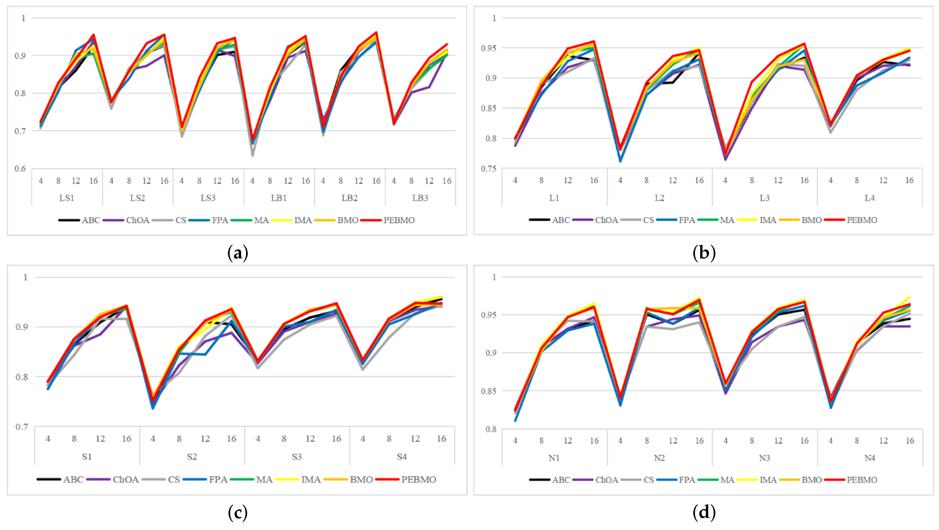
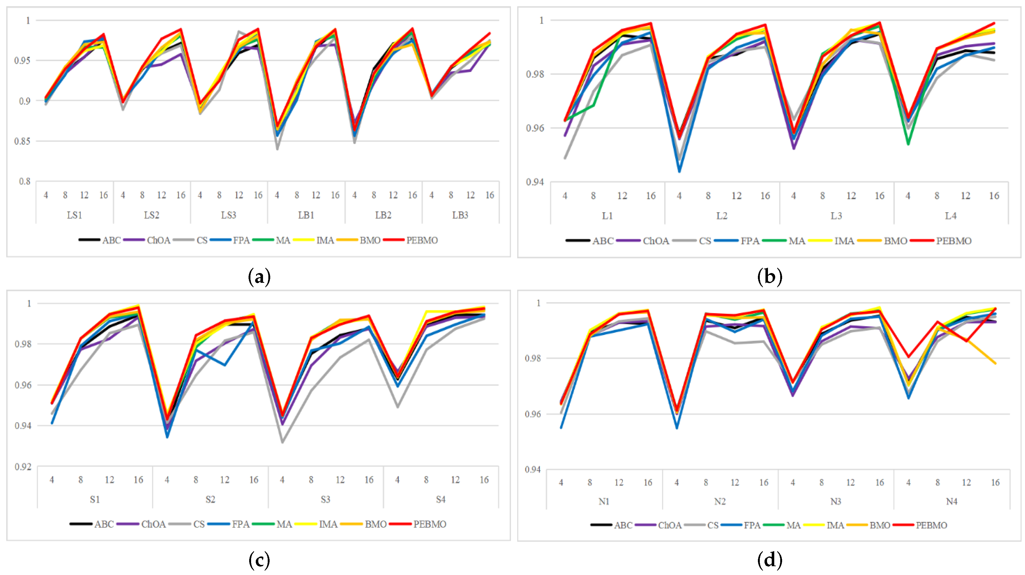
Feature similarity analysis: The optimal SSIM values obtained by ABC, ChOA, CS, FPA, MA, IMA, BMO, and PEBMO are 5, 3, 4, 3, 4, 19, 7, and 27, respectively. Of which are 1, 1, 2, 2, 1, 1, 1, 3, and 13 on the non-uniform canopy images; on low-illumination canopy images are 1, 0, 1, 1, 1, 1, 3, 1, 8; on strong light canopy images are 2, 0, 1, 0, 1, 6, 2, 4; and on normal illumination canopy images are 1, 2, 0, 0, 1, 1, 9, 1, 2. Regarding the optimal SSIM values distribution, the overall IMA and PEBMO algorithms have a clear advantage, obtaining 63.89% of the optimal SSIM values. IMA’s strengths are centered on strong and normally illuminated canopy images, while the PEBMO algorithm outperforms the comparison algorithm on non-uniform and low-illumination canopy images. The performance of the other algorithms is rather mediocre.

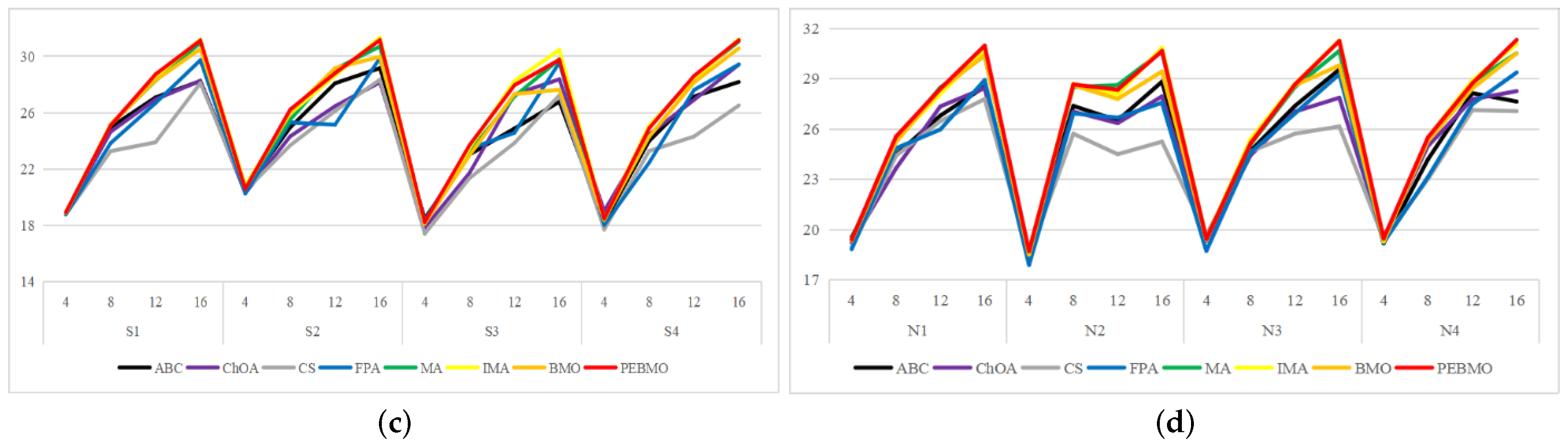
Degree of image distortion: the ABC, ChOA, CS, PFA, MA, IMA, BMO, and PEBMO algorithms obtained 4, 2, 4, 3, 5, 19, 6, and 29 optimal PSNR values, respectively. The IMA and PEBMO algorithms outperformed the others, indicating that their segmented canopy images were less distorted and of better quality. The performance of the algorithms on non-uniform canopy images is more balanced. The PEBMO algorithm obtains 10 out of 24 optimal values on non-uniform canopy images, which is slightly better than the comparison algorithms. The PEBMO algorithm has a clear advantage in low-illumination canopy images, obtaining 62.5% of the optimal PSNR values. In contrast, the MA and CS algorithms are slightly inferior, obtaining two optimal values, respectively. In the strong and normal illumination images, the IMA algorithm obtained 14 optimal values, while the PEBMO algorithm obtained 8, indicating that the IMA algorithm segmented images with better quality.

Feature similarity analysis: 6.94%, 2.78%, 2.78%, 5.56%, 9.72%, 15.28%, 30.56%, and 33.33% of the optimal FSIM values were obtained for ABC, ChOA, CS, FPA, MA, BMO, IMA and PEBMO, respectively. MA and BMO algorithms outperform ABC, ChOA, CS, and FPA, which indicates that they also have good optimization-seeking performance. IMA and PEBMO improve the FSIM values of both MA and BMO by 73.61%. Therefore, it is essential to increase the feature similarity between the segmentated canopy image and the original one by improving the performance of the intelligent algorithms.

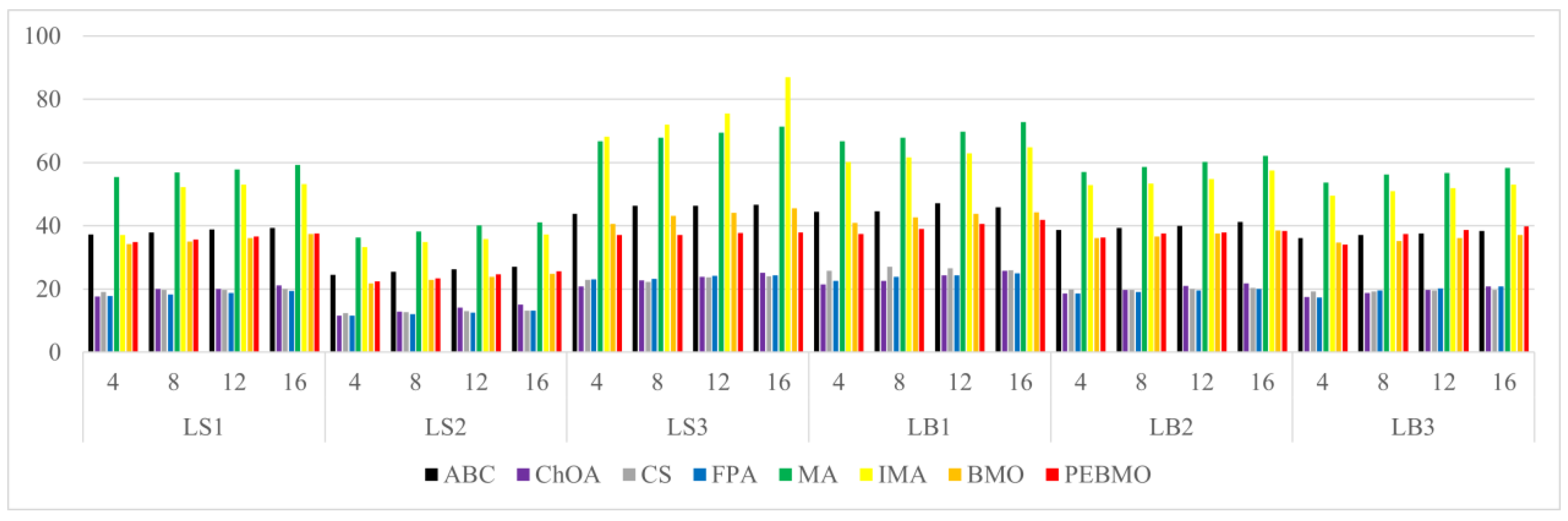
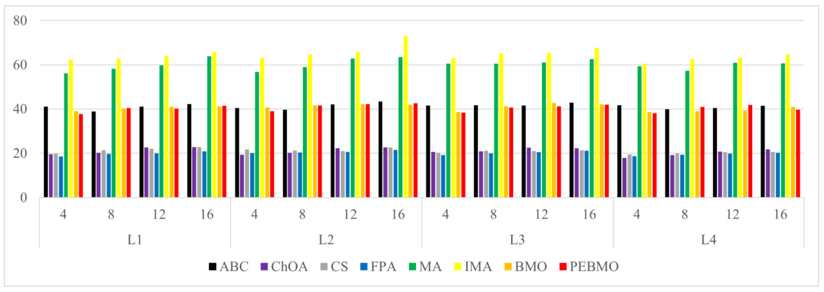
Image segmentation efficiency: by analyzing the computation time data of each algorithm, it can be concluded that all algorithms take no more than 5s when the number of thresholds increases from 4 to 16. The limitation that the computational complexity increases exponentially with increasing the number of thresholds in multi-threshold segmentation is overcome. The FPA, CS, and ChOA algorithms have apparent advantages. The MA and IMA algorithms have the lowest segmentation efficiency, which is inferior to the others. The gap between the BMO and PEBMO algorithms is not large, which suggests that improving the PEBMO algorithm does not increase the segmentation efficiency of the BMO algorithm. The segmentation efficiency of ABC is between that of PEBMO and MA.

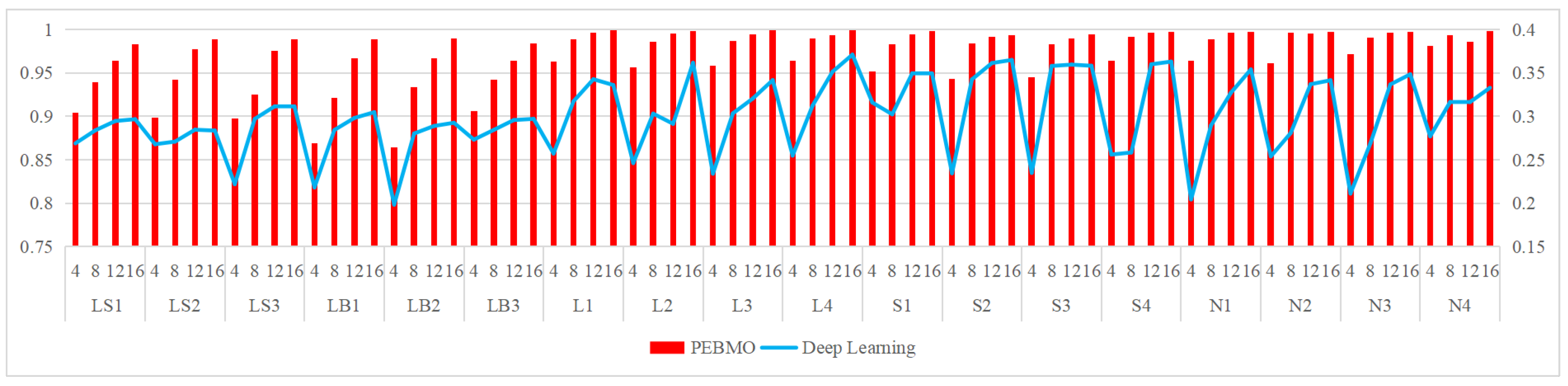
Comparison with deep learning segmentation methods: in comparison with deep learning methods, the PEBMO algorithm outperforms deep learning methods in terms of fitness value, standard deviation value, FSIM, and computation time, while deep learning outperforms the PEBMO algorithm in terms of SSIM and PSNR. Both algorithms have advantages and disadvantages. Deep learning has a clear advantage in segmentation quality. However, it also has the limitations of poor stability and high data dependency. The PEBMO algorithm, on the contrary, is stable, computationally efficient, and easy to implement. Still, it also suffers from significant performance degradation in low-dimensional or complex cases and high distortion.

In further research, overall, the PBEMO algorithm is better than the IMA algorithm, but its advantage is mainly concentrated in non-uniform and low-illumination canopy images. The IMA algorithm is 53.126% better than the PEBMO algorithm in segmenting normal illumination and strong illumination images. Therefore, further improvement of the BMO algorithm is necessary to improve its segmentation accuracy on high-brightness canopy images. In addition, this study provides a comprehensive comparison with the deep learning segmentation method, in which both algorithms have strengths and weaknesses. Deep learning has apparent advantages in segmentation quality. However, it also has the limitations of poor stability and excessive dependence on data, while the PEBMO algorithm is the opposite, with good stability, high computational efficiency, and ease of implementation. Therefore, different segmentation methods can be used based on these requirements.

5. Conclusions

This paper proposes a method to segment forest canopy images using Kapur entropy combined with the PEBMO algorithm. Compared with the segmentation results of ABC, ChOA, CS, FPA, MA, IMA, and BMO, the segmentation efficiency of the PEBMO algorithm is not as good as that of ChOA, CS, and FPA. Still, it has apparent advantages in segmentation accuracy and stability. The PEBOM and BMO algorithms are not significantly different in segmentation efficiency, which indicates that the improvement of the PEBMO algorithm does not increase the complexity of the BMO algorithm. In addition, the PEBMO algorithm was comprehensively compared with the deep learning segmentation method. The PEBMO algorithm is superior to the deep learning method in terms of the segmentation accuracy, stability, feature similarity, and efficiency. In contrast, the deep learning method was superior to the PEBMO algorithm in terms of structural similarity and image distortion. The two segmentation methods are short. Because this study only focused on small samples of canopy images, it lacked practical validation using large-scale datasets. In contrast, deep learning-based segmentation methods have the advantage of handling large-scale datasets.